The apparent focal depth, emergence angle, and take-off angle of seismic wave measured by YRY-4-type borehole strainmeter as one kind of strain seismograph

1 Introduction

Since the 1960s, relative stress observations have been carried out in the United States, China, Japan and other countries (Sacks et al., 1971; Gladwin, 1984; Ishii, 2001); borehole strain observation is a vital observation method gradually developed from relative stress observation. Scholars in mainland China have developed RZB-type four-component borehole strainmeter (Ouyang, 1977), TJ-type borehole volume strainmeter (Su, 1982), and YRY-type four-component borehole strainmeter (Chi et al., 2009), and continuously improved the observation technology. It has developed to more than 130 stations equipped with borehole strainmeters. These borehole strain observations can record clear solid tides and play an essential role in the field of earthquake monitoring and prediction in mainland China (Huang et al., 2017).

Unlike GTSM strainmeter such as the United States, which can produce high frequency data of 20 Hz, the data sampling rate of strainmeter in mainland China is minute sampling due to data storage and transmission technology. Using these minute data, scholars in mainland China have carried out a lot of research, including the tidal Variation and calibration technology (Qiu et al., 2015), abnormal changes of different earthquakes (Qiu et al., 2010; Liu et al., 2014), co-seismic strain steps (Gong et al., 2019; Li et al., 2020), free oscillation of the earth excited by large earthquakes (Tang et al., 2007; Tang et al., 2008; Qiu, 2017), and also studied and analyzed the influence of water level, air pressure, rainfall and other factors on borehole strain, and studied the data processing methods to identify and eliminate these influencing factors (Zhou et al., 2008; Zhang and Huang, 2011; Zhang et al., 2015). However, these studies are limited to longer period signals because of the low sampling rate.

Numerous studies have shown that the borehole strainmeter can be used for seismic wave observation (Byerly, 1926; Johnston et al., 1986; Borcherdt and Glassmoyer, 1989; Borcherdt et al., 2006; Johnston et al., 2006; Blum et al., 2010; Barbour and Agnew, 2012; Qiu et al., 2015; Barbour and Crowell, 2017; Canitano et al., 2017; Cao et al., 2018; Farghal et al., 2020; Barbour et al., 2021). This initially realized seismologists’ expectations of strain seismographs (Benioff et al., 1961; Aki and Richards, 2002). Although the current horizontal component borehole strainmeter can only detect the two-dimensional strain variation in the horizontal plane, the seismic wave is usually approximated as a plane wave, and both have only three independent components, which can convert to each other. Therefore, this instrument can still be used to observe and analyze the strain variation of seismic waves.

Notably, strain seismographs are different from traditional pendulum seismographs. The traditional pendulum seismograph measures a vector (displacement), while the strain seismograph detects a tensor (displacement gradient). The strain seismograph can provide new information that can be used to carry out further research. One of the most critical research directions is the inversion of focal mechanism with strain seismic observation. Theoretically, the source moment tensor (Qiu et al., 2020) can be converted from the data of at least two strain observation points in different directions. Solving the focal mechanisms of local earthquakes by strain seismic observation can be used as supplementary information for pendulum seismograph observation.

The determination of the focal mechanism by seismic strain observation is theoretically based on the assumption of an ideal homogeneous medium, but the actual crustal strata are inhomogeneous. Figure 1 shows the geometrical interpretation of seismic wave propagation in homogeneous and inhomogeneous media. In a homogeneous medium, the angle (take-off angle) i_e between the seismic wave ray from the hypocenter and the normal direction of the ground remains unchanged when the seismic wave propagates linearly, which is equal to the emergence angle i₀ when reaching the ground. Seismic waves propagating in non-uniform strata can reflect and refract, and the rays are not straight lines. When the focal depth cannot be ignored, the emergence angle i is generally not equal to the take-off angle, i_e. This makes it difficult to solve the focal mechanism by seismic strain observation. The crust is separated from the mantle by the Moho surface, and it can be considered that there is no similar interface within the crust (Wyllie PJ, 1963). However, crustal rock is not a homogeneous medium. Basically, the wave velocity generally linearly increases with depth. As a first-order approximation, it can be considered that the gradient of wave velocity of crustal rocks with depth is a constant; this is defined as a constant velocity gradient model (Stein and Wysession, 2003; Wan, 2016). Under this condition, for local earthquakes, when the observation site is very close to the epicenter (within tens of kilometers), because the seismic waves only propagate in the crust, the initial motion is a direct wave, so the situation becomes relatively simple.

FIGURE 1

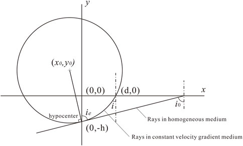
FIGURE 1. The geometry of the constant velocity gradient model. i_e: take-off angle; i: emergence angle for constant velocity gradient medium; i₀: emergence angle for homogeneous medium; (d, 0): site coordinates; (0, h): focal coordinates.

As the technical management and planning team of the borehole strain network in Mainland China, we have upgraded and updated the high-sampling data collectors of 10 four-component borehole strainmeters which are producing high frequency data of 100 Hz since 2017, only one site could produce high-frequency data before. Using these data, the ability of four-component borehole strainmeters to record strain seismic waves of earthquakes of different magnitudes has been studied (Qiu et al., 2015; Tang et al., 2022), the study of determining the strain magnitude of seismic surface wave based on borehole strain seismic wave is carried out (Li et al., 2020), Shi et al. (2021) studied the direct observation of co-seismic static stress deviation changes consistent with the theoretical prediction. These sites can record the seismic waves of earthquakes with M6.0 or above in the world (Tang et al., 2022), and can also record the local earthquakes in the area where the site is located. In this article, two earthquakes are experimentally examined through seismic strain observation using a high-density borehole strainmeter network in Xinzhou, Shanxi Province, China. The results show that there is an obvious rule that the emergence angle of seismic waves reaching the observation sites varies with the epicentral distance, which can be simulated by the crustal wave velocity structure model with constant velocity gradient. On this basis, not only the focal depth can be calculated, the take-off angle of seismic wave rays arriving at each observation site can be determined.

2 Data

YRY-4 type of four-gauge borehole strainmeter (FGBS) is an important instrument for crustal deformation observation in china; the overall composition of the borehole observation (Tang et al., 2020) was designed by us as the drafters for the construction of the seismic industry standard borehole strain stations in mainland China and the four sensors of the YRY-4- type FGBS (Qiu et al., 2013; Li et al., 2021) are shown in Figure 2. The four gauges are arranged at 45° intervals, Si (i =1, 2, 3, 4) is the measurement obtained from each of the four gauges; it directly measure the change in diameter in the corresponding azimuth that results from changes in strain state. Since 2012, the YRY-4 -type FGBS has been used in Xinzhou area of Shanxi Province, and the sites such as Shenchi (SC), Fanshi (FS), Yuanping (YP), Daixian (DX), and Ningwu (NW) have been successively established, forming a high-density local observation network, as shown in Figure 3, and the measurement information of 5 sites are in Table 1. In 2018, we conducted an earthquake monitoring experiment using this observation network with a sampling rate of 100 Hz. Presently, more than 2 years of data have been accumulated. We have been very fortunate to capture two small local seismic events (YP M2.8 and DX M3.0) within the observation network (Figure 3), Table 2 gives the parameters of the two local events calculated by traditional pendulum seismograph, which are provided by the China Seismic Network.

FIGURE 2

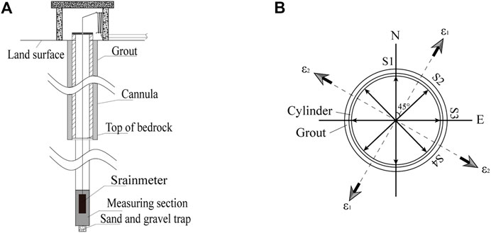
FIGURE 2. (A)The overall composition diagram of a standard borehole strain observation; (B) Schematic diagram of a standard borehole strainmeter, S1, S2, S3, S4 sensors in 4 directions,ε₁ and ε₂ represent the maximum and minimum principal strains, respectively.

FIGURE 3

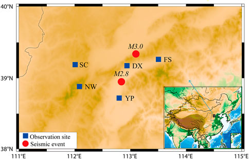
FIGURE 3. Map of the observation sites and the two local events.

TABLE 1

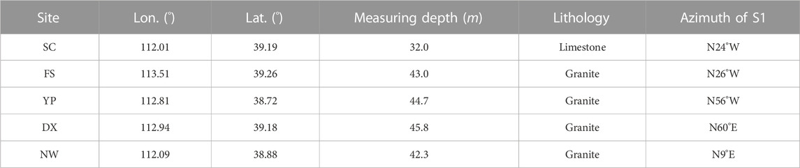
TABLE 1. Measurement information of 5 sites.

TABLE 2

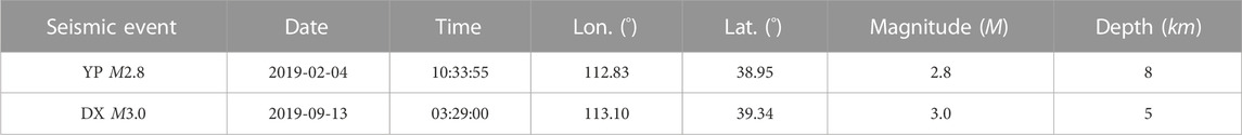
TABLE 2. Parameters of the two local events provided by the China Seismic Network.

YRY-4-type FGBS has good observation performance and has achieved great success in the study of geodynamic problems (Chi et al., 2009; Qiu et al., 2013; Liu et al., 2014). Some scholars have also studied the theoretical issues and feasibility of using the observed seismic strain waves (Zhang et al., 2019; Zhang et al., 2020; Zhang et al., 2021), but there has been no actual observation to verify the results. For the two earthquakes, the P and S waves of seismic strain waves recorded by the YRY-4-type FGBS at all the sites are apparent in Figure 4.

FIGURE 4

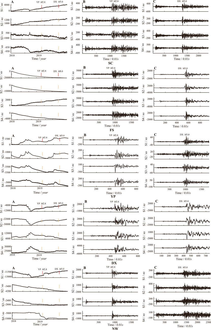
FIGURE 4. (A) Observation curves recorded by 5 sites in 2018-2019; (B) P and S waves of YP M2.8 event observed at 5 sites; (C) P and S waves of DX M3.0 event observed at 5 sites.

Based on NW in Figure 4, Figure 5 shows the more apparent seismic wave curve of YP M2.8 earthquake recorded at the NW site. For such local earthquakes, the first pulse (direct wave P_g and S_g) reaching the observation site is the most direct reflection of the earthquake hypocenter, which is extremely valuable for examining the focal mechanism. In this article, the extreme value (wave peak or trough) of this pulse is called the initial motion. The arrow in Figure 5 indicates the selection time of direct strain wave observation data.

FIGURE 5

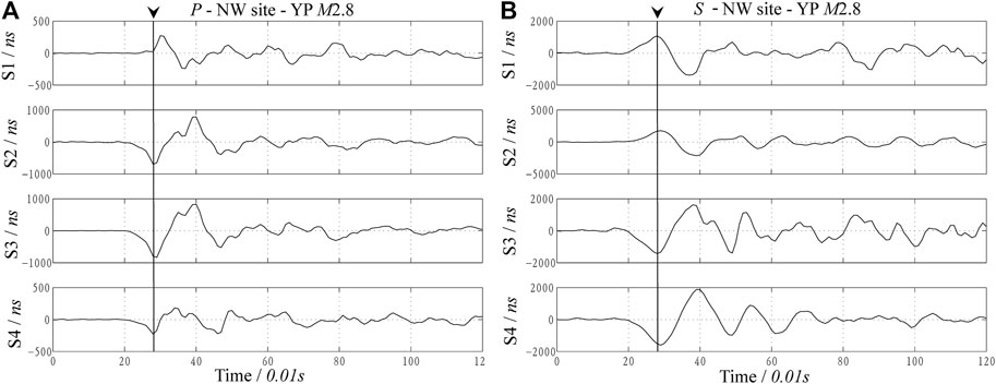
FIGURE 5. P (A) and S (B) waves of the M2.8 event were observed at the NW site.

It should be noted that the observation curve in Figure 5 does not show the real strain variation. The borehole strainmeter directly measures the relative diameter change of the probe sleeve, which requires calibration and conversion to obtain the strain variation in the rock layer (Qiu et al., 2013). The long-period signals, such as hydrological and tidal effects have no effect on high-frequency seismic wave signals, so it is reasonable to remove the linear trend of the observed record only by fitting. Table 3 and Table 4 show the observed strains of the initial motions of P and S waves of the two earthquakes in Table 2. ${\epsilon }_{11}$, ${\epsilon }_{12}$, and ${\epsilon }_{22}$ are three strain components in the horizontal plane of the geographic coordinate system obtained by calibration and conversion.

TABLE 3

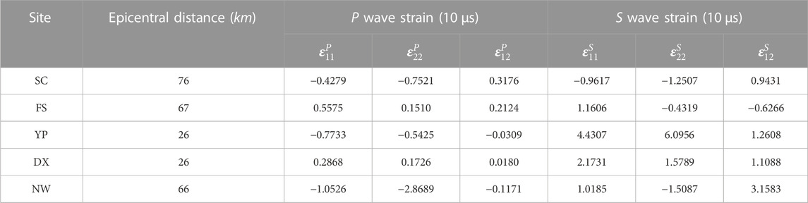
TABLE 3. Observed strains of the initial motions of P and S waves for the M2.8 event.

TABLE 4

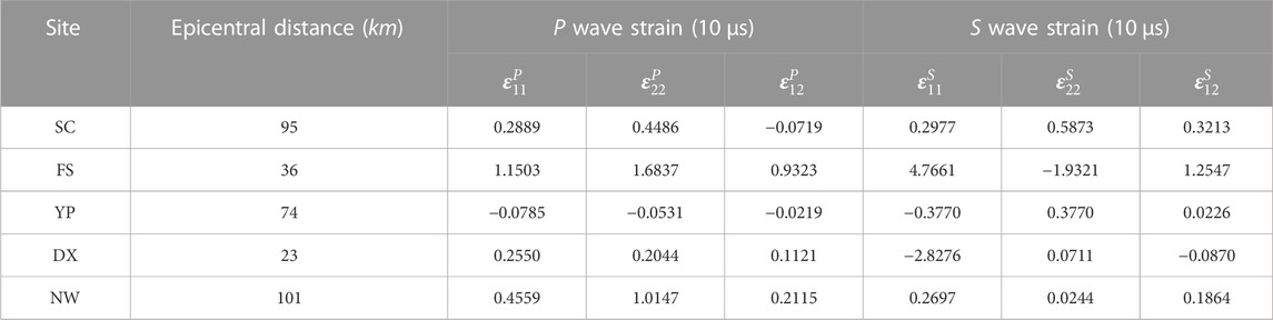
TABLE 4. Observed strains of the initial motions of P and S waves for the M3.0 event.

3 Methods and models

3.1 Strain conversion of emergent wave

3.1.1 Hypothesis

To discuss the evaluation of actual seismic wave strain using the observed horizontal strain, there are some hypotheses: Firstly, it is assumed that the epicenter location is known. Since Shanxi Province has a relatively dense pendulum seismograph observation network, it can be considered that this epicenter location is reliable. Secondly, the seismic wave near the earthquake hypocenter must not be an ideal plane wave, but the seismic wave reaching the observation site can be treated as a plane wave. Finally, the local earthquake events are discussed here, so it can be assumed that the path deviations of the P wave and S wave from the source to the observation site are small, which can be regarded as approximate values (Qiu et al., 2020). Practical calculations also confirm these hypotheses.

3.1.2 Fundamental formula

In the geographic coordinate system shown in Figure 6, the strain tensor of the seismic waves arriving at the observation site is denoted as

${\epsilon }_G=\left[\begin{array}{ccc}{\epsilon }_{11}& {\epsilon }_{12}& {\epsilon }_{13}\\ {\epsilon }_{12}& {\epsilon }_{22}& {\epsilon }_{23}\\ {\epsilon }_{13}& {\epsilon }_{23}& {\epsilon }_{33}\end{array}\right](1)$

FIGURE 6

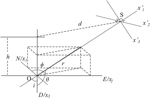
FIGURE 6. Geographical coordinates (x₁, x₂, x₃) and ray coordinates (x’₁, x’₂, x’₃). “O” represents the seismic focus; “S” represents the seismographic site.

However, the current borehole strainmeter can only observe symmetrical horizontal strain variation, i.e., only the three independent strain components (ε₁₁, ε₁₂, and ε₂₂) shown in the dashed frame of Eq. 1, the vertical strain components (ε₁₃, ε₂₃, and ε₃₃) are not considered.

According to the above assumptions, the seismic waves reaching the observation site can be regarded as plane waves. In the seismic ray coordinate system shown in Figure 6, where the seismic waves propagate along the x’₁ axis, the strain tensor should be written as (Qiu, 2017)

$\begin{array}{l}{\epsilon }_R={\epsilon }_R^P+{\epsilon }_R^{SH}+{\epsilon }_R^{SV}\\ =\left[\begin{array}{ccc}{\epsilon }_{11}^{\prime }& 0& 0\\ 0& 0& 0\\ 0& 0& 0\end{array}\right]+\left[\begin{array}{ccc}0& {\epsilon }_{12}^{\prime }& 0\\ 0& 0& 0\\ 0& 0& 0\end{array}\right]+\left[\begin{array}{ccc}0& 0& {\epsilon }_{13}^{\prime }\\ 0& 0& 0\\ 0& 0& 0\end{array}\right],\\ =\left[\begin{array}{ccc}{\epsilon }_{11}^{\prime }& {\epsilon }_{12}^{\prime }& {\epsilon }_{13}^{\prime }\\ 0& 0& 0\\ 0& 0& 0\end{array}\right]\end{array}(2)$

where ${\epsilon }_R^P$ is the P wave strain, ${\epsilon }_R^{SH}$ is the SH wave strain, and ${\epsilon }_R^{SV}$ is the SV wave strain. It should be noted that ${\epsilon }_{12}^{\prime }$ is parallel to the ground, while ${\epsilon }_{13}^{\prime }$ is perpendicular to the ground. It is also noteworthy that ${\epsilon }_R$ is asymmetric.

The relationship between the horizontal strain detected at the observation site and the actual plane seismic wave strain should conform to the following coordinate transformation equation:

${\epsilon }_G=l_{GR}{\epsilon }_R{l}_{GR}^T(3)$

where the direction chord matrix is defined as follows:

$l_{GR}=\left[\begin{array}{ccc}{l}_{11}& l_{12}& l_{13}\\ l_{21}& l_{22}& l_{23}\\ l_{31}& l_{32}& l_{33}\end{array}\right](4)$

The column vectors of $l_{GR}$ are the direction vectors of the axes of the seismic wave ray coordinate system (x’₁, x’₂, x’₃) in the geographic coordinate system (x₁, x₂, x₃).

In fact, P and S waves propagate separately, while SH and SV waves propagate together. For P waves, for the strain component that can be observed by the borehole strainmeter, Eq. 3 can be written as follows:

$\left\{\begin{array}{l}{\epsilon }_{11}^P={\epsilon }_{11}^{\prime }{l_{11}}^2\\ {\epsilon }_{22}^P={\epsilon }_{11}^{\prime }{l_{21}}^2\\ {\epsilon }_{12}^P={\epsilon }_{11}^{\prime }{l}_{11}{l}_{21}\end{array}\right.(5)$

The ${\epsilon }_{11}^{\prime }$ of the observation site can be calculated by Eq. 5. For S wave, Eq. 3 can be written as

$\left\{\begin{array}{l}{\epsilon }_{11}^S=2{\epsilon }_{12}^{\prime }{l}_{11}{l}_{12}+2{\epsilon }_{13}^{\prime }{l}_{13}{l}_{11}\\ {\epsilon }_{22}^S=2{\epsilon }_{12}^{\prime }{l}_{21}{l}_{22}+2{\epsilon }_{13}^{\prime }{l}_{23}{l}_{21}\\ {\epsilon }_{12}^S={\epsilon }_{12}^{\prime }\left(l_{11}{l}_{22}+l_{12}{l}_{21}\right)+{\epsilon }_{13}^{\prime }\left(l_{13}{l}_{21}+l_{11}{l}_{23}\right)\end{array}\right.(6)$

${\epsilon }_{12}^{\prime }$ and ${\epsilon }_{13}^{\prime }$ of the observation site can be calculated from Eq. 6.

As shown in Figure 6, the emergence angle is expressed as $i=\pi -\theta$. The components of $l_{GR}$ can be expressed by azimuth angle $\phi$ and emergence angle i:

$\left\{\begin{array}{l}{l}_{11}=\sin i\cos \phi \\ l_{21}=\sin i\sin \phi \\ l_{31}=-\cos i\\ l_{12}=-\sin \phi \\ l_{22}=\cos \phi \\ l_{32}=0\\ l_{13}=-\cos i\cos \phi \\ l_{23}=-\cos i\sin \phi \\ l_{33}=\sin i\end{array}\right.(7)$

3.1.3 Practical algorithm

In addition to the known observations, the azimuth $\phi$ can be calculated from the epicenter position for an observation site. In other words, we are facing with an overdetermined problem; four unknowns need to be solved by Eqs 5, 6: ${\epsilon }_{11}^{\prime }$ , ${\epsilon }_{12}^{\prime }$ , ${\epsilon }_{13}^{\prime }$ , and the emergence angle i.

In a homogeneous medium, if the epicentral distance d and focal depth h are known, the emergence angle i can be easily calculated. However, on the one hand, although the epicentral distance d is generally reliable, the focal depth h given by the existing methods is not reliable; on the other hand, the crustal strata are not a homogeneous medium. Therefore, the emergence angle i cannot be given in advance.

Here, the apparent focal depth at each observation site is defined as

$h_i=\frac{d}{\tan i}(8)$

We first calculate the apparent focal depth h_i rather than the emergence angle i. Because the focal depth is not a high-precision quantity, it is generally accurate to the km level. Therefore, we use the enumeration method, where all the values from 1 km to 300 km are tried, and the optimal value is selected as the apparent focal depth; the error does not exceed 1 km.

For an observation site, we proposed a specific algorithm to determine the focal depth as follows. Firstly, for the attempted h_i, three ${\epsilon }_{11}^{\prime }$ are obtained by using Eq. 5, and the standard deviation $std\left({\epsilon }_{11}^{\prime }\right)$ is calculated. Secondly, for the attempted h_i, three ${\epsilon }_{12}^{\prime }$ and three ${\epsilon }_{13}^{\prime }$ are obtained by using Eq. 6, and the corresponding standard deviations $std\left({\epsilon }_{12}^{\prime }\right)$ and $std\left({\epsilon }_{13}^{\prime }\right)$ are calculated. Thirdly, the objective function is established as follows:

$F_{std}=\log \left[std\left({\epsilon }_{11}^{\prime }\right)+std\left({\epsilon }_{12}^{\prime }\right)+std\left({\epsilon }_{13}^{\prime }\right)\right](9)$

Finally, all h_i are tested, and the minimum target function h_i is selected as the apparent focal depth of the observation point. Further, the corresponding ${\epsilon }_{11}^{\prime }$, ${\epsilon }_{12}^{\prime }$, and ${\epsilon }_{13}^{\prime }$ are selected as the strain component value of the plane seismic wave reaching the observation site.

For the two earthquakes, Figure 7 shows the calculated apparent focal depth of the five observation sites. There are two notable points. First, the objective function can reach the obvious minimum extreme point; second, as shown in the sub-graphs at the lower right corner of Figures 7A, B, compared with Figure 3 and Table 3, and Table 4, the apparent focal depth of each observation site shows linear behavior: when the epicentral distance is larger, the apparent focal depth is also larger. These two points prove the reliability of the observation data as well as the accuracy of the calculation results. Further, the calculation results validate the feasibility of the above-mentioned assumptions.

FIGURE 7

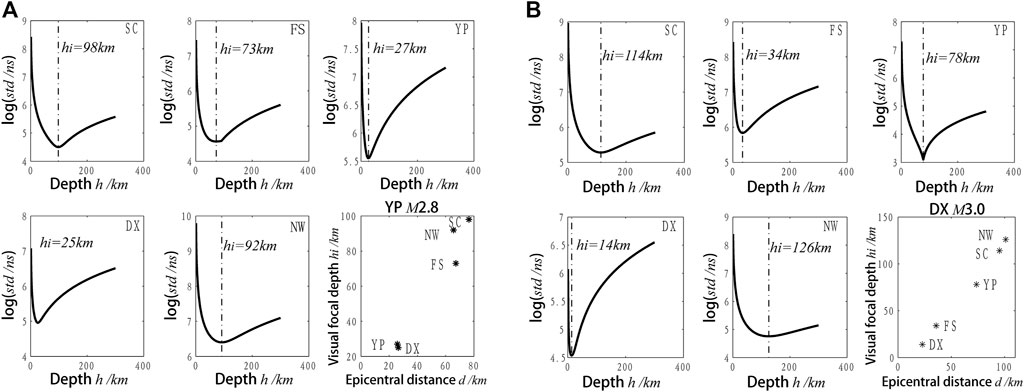
FIGURE 7. Optimal estimations of the apparent focal depths (indicated by the dash-dotted lines) for the two events: (A) YP M2.8, (B) DX M3.0.

3.2 Constant velocity gradient model

The two earthquakes recorded by our experimental network occurred in the crust. In a homogeneous medium, seismic waves should propagate linearly. If the crust is a homogeneous medium, the apparent focal depth calculated at all the observation sites should be equal to the actual focal depth when the seismic wave emitted by the hypocenter reaches different observation sites. However, actually, the apparent focal depths of each observation site are different, indicating that the crust may not be homogeneous medium.

The variation in the wave velocity of crustal rocks with depth is very complex, but the primary feature of the crustal structure is that the wave velocity increases with depth. As a first-order approximation, we can consider that the wave velocity steadily increases with depth, which is called the constant velocity gradient model (Stein and Wysession, 2003; Wan, 2016). When the epicentral distance is larger, the observed phenomenon that the focal depth is larger can be explained by this model.

The constant wave velocity gradient model is usually established on the premise that the hypocenter is located on the surface. To examine the seismic wave rays of local earthquakes, the constant velocity gradient model with a certain depth is considered, as shown in Figure 1. Assuming that the wave velocity gradient is k, the variation in the wave velocity with depth can be expressed as follows:

$v=v_e-k\left(y+h\right)=v_0-ky(10)$

where $v_e$ is the wave velocity at the focal depth, and $v_0=v_e-kh$ is the wave velocity near the surface. In a homogeneous medium, the rays emitted from the take-off angle $i_e$ propagate in a straight line, and the emergence angle $i_0=i_e$ reaches the surface. In the medium, where the wave velocity steadily increases with depth, the emergence angle $i\ne i_e$ reaches the surface.

The characteristic of the rays emitted from the emergence angle $i_e$ is that the radius of curvature $\rho$ remains constant (Wan, 2016), which can be written as

$\rho =\frac{1}{pk}(11)$

where p is the ray parameter, which conforms to Snell’s law as follows:

$p=\frac{\sin i_e}{v_e}(12)$

According to the previous assumptions, the path of P and S waves is the same, i.e., p is the same. Substituting Eq. 12 into Eq. 11, we get

$\rho =\frac{H}{\sin i_e}(13)$

where $H=\frac{v_e}{k}$, H reflects the relationship between wave velocity gradient and wave velocity at the focal depth.

3.3 Formula of take-off angle

As mentioned above, in a constant velocity gradient medium, the equation of the circle (Figure 1) of the seismic wave rays emitted from the source is as follows:

${\left(x-x_0\right)}^2+{\left(y-y_0\right)}^2={\rho }^2(14)$

where

$\left\{\begin{array}{l}{x}_0=-\rho \cos i_e\\ y_0+h=\rho \sin i_e\end{array}\right.(15)$

On the ground, y = 0. Substituting Eq. 15 into Eq. 14 and simplifying it, we get

$x^2+2x\rho \cos i_e+h^2-2h\rho \sin i_e=0(16)$

Then, inserting Eq. 13 with Eq. 16, we obtain

$x^2+2x\frac{H}{\tan i_e}+h^2-2hH=0(17)$

Thus, the take-off angle can be expressed as

$i_e=\arctan \frac{2Hx}{2Hh-h^2-x^2}(18)$

where x is the epicentral distance, which can also be denoted by d.

Using Eqs 14, 15 we get

$y=\pm \sqrt{{\rho }^2-{\left(x+\rho \cos i_e\right)}^2}+\rho \sin i_e-h(19)$

Then, the actual seismic wave ray equation can be written as

$\begin{array}{l}y=-\sqrt{{\rho }^2-{\left(x+\rho \cos i_e\right)}^2}+\rho \sin i_e-h\\ =-\sqrt{\frac{H^2}{{\sin }^2{i}_e}-{\left(x+\frac{H}{\tan i_e}\right)}^2}+H-h\end{array}(20)$

Using Eq. 20, seismic wave rays with different departure angles can be obtained. Differentiating the above equation to x and substituting Eq. 13 into it, we get

$\frac{dy}{dx}=\frac{x+\rho \cos i_e}{\sqrt{{\rho }^2-{\left(x+\rho \cos i_e\right)}^2}}(21)$

Finally, using Eqs 13, 18, we get

$\frac{dy}{dx}=\frac{2h\left(H-h\right)+x^2}{2\left(H-h\right)x}(22)$

The emergence angle of seismic waves reaching the observation site is expressed as

$i=\frac{\pi }{2}-\arctan \frac{dy}{dx}(23)$

4 Results and discussion

4.1 Fitting results

The feasibility of using the constant velocity gradient model to explain the actual observation results depends on whether the emergence angle of each observation site can be approximately fitted with Eq. 22. The observation Eq. 22 and related Eqs 21, 18 involve two quantities with clear physical significance: focal depth h and take-off angle, i_e, which are the quantities to be determined through the fitting.

Equation 22 gives the emergence angle i corresponding to different epicentral distances x. To explain our experimental results, we must determine two parameters in Eq. 22: h and H, where the focal depth h has a more significant application value.

This problem is non-linear, and the enumeration method is still used for inversion. For the focal depth h, all the integer values from 1 km to 100 km are traversed, and the error does not exceed 1 km. Since v_e generally does not exceed 8 km/s in the crust, assuming that the wave velocity near the surface is 5 km/s and the crustal thickness is 30 km, then k is approximately 0.1/s, and the corresponding H is equal to 80 km. Based on this analysis, the variation range of H is selected as 1-200 km, and all the integer values are traversed with an error of less than 1 km. The specific algorithm is as follows. Firstly, the given h and H values are substituted into Eq. 22 to establish the x-i relation. Secondly, the epicentral distance of each observation site of j is replaced into the established x-i relationship; the emergence angle $i_j^{\prime }$ is calculated and compared with the actual observed emergence angle $i_j$. Thirdly, the objective function: $F={\displaystyle \sum }_{j=1}^5\left|i_j-i_j^{\prime }\right|$, is established. Finally, all the h and H values are traversed, and the h and H values that minimize the objective function F are selected as the solution. The corresponding x-i relationship is considered as the criterion.

Figure 8 shows the fitting results of two earthquakes. Here, the dash-dotted curve shows the variation in the emergence angle with the epicentral distance in the homogeneous medium under the same focal depth. The solid curve is the x-i relationship obtained by the constant velocity gradient model. Obviously, the observed x-i relationship does not conform to the homogeneous medium model, but it is in good agreement with the constant velocity gradient model. The inversion results of h and H are also shown in Figure 8, which shows that the focal depths h of the two earthquakes is 11km and 7 km respectively, which are consistent with the results of 8km and 5 km given by the pendulum seismograph (Table 2). It is noteworthy that the H of the two local events is 48 km and 49 km, respectively, and the results are largely consistent; this also explains that the medium structure should also be consistent results for two earthquakes in the same area.

FIGURE 8

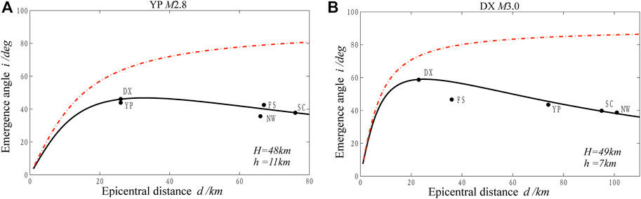
FIGURE 8. Calculated emergence angle (i) vs. epicentral distance (d) of the two events: (A) YP M2.8, (B) DX M3.0.

Red dash-dotted line: homogeneous medium; solid line: constant velocity gradient medium.

Once h and H are determined, seismic wave rays can be plotted for different take-off angles, as shown in Figure 9 (solid lines). It is also necessary to give the take-off angle corresponding to each observation site to plot the seismic wave rays at each observation site, which are shown by red dash-dotted lines in Figure 9.

FIGURE 9

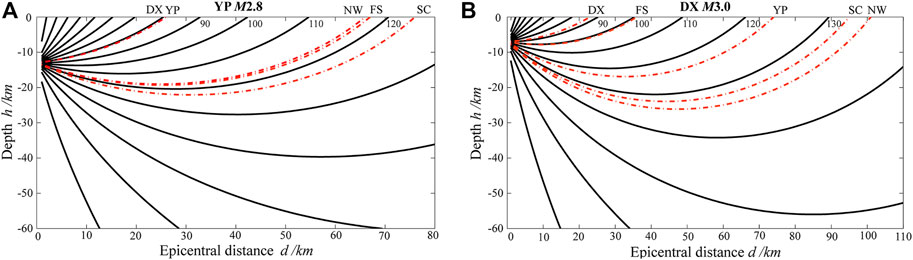
FIGURE 9. Ray paths of the two events according to constant velocity gradient model: (A) YP M2.8, (A) DX M3.0.

Eq. 21 can be rewritten as

$\cot i=\frac{x+\rho \cos i_e}{\sqrt{{\rho }^2-{\left(x+\rho \cos i_e\right)}^2}}(24)$

Squaring and expanding both sides of Eq. 24, we obtain

${\rho }^2{\cot }^{2}i=\left(1+{\cot }^{2}i\right){\left(x+\rho \cos i_e\right)}^2(25)$

Using trigonometric function relation, we get

$\frac{{\cot }^{2}i}{1+{\cot }^{2}i}={\cos }^{2}i(26)$

Substituting Eq. 14 into Eq. 25 (y = 0 on the ground), we have

${\rho }^2{\cos }^{2}i={\rho }^2-{\left(\rho \sin i_e-h\right)}^2(27)$

Then,

${\rho }^2{\sin }^{2}i={\left(\rho \sin i_e-h\right)}^2(28)$

Squaring both sides of Eq. 28 and substituting in Eq. 13, we get

$\frac{\sin i}{\sin i_e}=\pm \frac{H-h}{H}=\pm \frac{v_e-kh}{v_e}(29)$

Using Eq. 29, the following expression of Snell’s law can be obtained:

$\frac{\sin i_e}{v_e}=\pm \frac{\sin i}{v_0}(30)$

When h and H are known, $\frac{H-h}{H}$ can be calculated, and then the take-off angle, i_e is calculated from the emergence angle i according to Eq. 29. According to Figure 6, $i_e<{90}^{\circ }$ corresponds to the usual Snell’s law, where Eq. 30 takes a positive sign on the right. When $i_e>{90}^{\circ }$, the seismic waves emitted from the source are downward, and the negative sign should be taken. At the same time, the obtained negative take-off angle should be added to 180°. Eq. 18 shows that when $i_e={90}^{\circ }$, the epicentral distance is expressed as follows:

$x_{90}=\sqrt{2Hh-h^2}(31)$

Therefore, the epicentral distance is positive when $x<x_{90}$, and it is negative when $x>x_{90}$. In fact, the take-off angle can be directly calculated using Eq. 18. The two methods give the same results and substantiate each other. Table 5 shows the calculation results.

TABLE 5

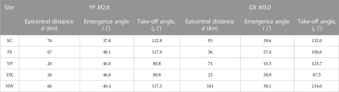
TABLE 5. Calculated emergence angles and take-off angles for the two local events.

It can be seen from Figure 9 that all the seismic wave rays represented by the dash-dotted lines do not exceed the depth of 30 km, and they should not exceed the crust range and are propagated in the crust.

4.2 Discussion

Most of the seismic sites and borehole strainmeter sites in mainland China are planned and constructed separately, so there are few sites where the two observations are co-located. Although Shanxi Province has a relatively dense pendulum seismograph observation network, there are only three seismic stations in the study area of this paper, and only the NW site is co-located. Seismic observation is a velocity observation optimized by frequency band; the strain observed by the four-component borehole strainmeter is a vector. The results of the two observations may be different. Therefore, the research in this paper did not carry out a detailed comparative analysis with seismic observations; only the hypocenter parameters given by the seismic network were compared. With continuous observation, the number of local earthquakes recorded has increased. In the future, we will use the sites where seismic and borehole strainmeters are co-located to carry out a comparative analysis of the two observations through a large number of earthquakes.

This study is part of our research on solving the focal mechanism solution with strain seismic observation, which broadens the application field of four-component borehole strain observation. The results can provide a practical basis for further development of the four-component borehole strainmeter in mainland China in the future. Other than that, some recent studies show that strain seismographs could help provide unique constraints for local earthquakes, which then further strengthening the efficiency of the local earthquake warning system (Juhel et al., 2018; Canitano et al., 2021). Based on the research in this paper, how to apply these high sampling sites to the earthquake early warning system in mainland China will be a meaningful study.

5 Conclusion

The apparent focal depth, the emergence angle, and the take-off angles of seismic waves given in this study for five sites of two local events have stable uniqueness and apparent regularity. In particular, the inverted focal depths are basically consistent with the interpretation results of the traditional pendulum seismograph, which shows the reliability of the research results. This provides another important application direction of the YRY-4 type four-gauge borehole strainmeter. The accuracy of the YRY-4 type four-gauge borehole strainmeter was the prerequisite for this study. The H values of the two earthquakes (H is the reflection of the relationship between wave velocity gradient and wave velocity at focal depth) are consistent, which also verifies the applicability of the crustal model with constant gradient wave velocity. The observation results suggest that the constant velocity gradient model is more realistic than the homogeneous medium crust model.

Currently, the research on solving focal mechanisms by seismic strain observation is limited to local earthquakes. Especially, in the range of direct wave with initial motion, the seismic moment is generally less than 100 km. At present, there is no good way to solve the problem that the emergence of the first wave and mantle reflection wave in a larger range can cause greater errors in the inversion. However, the research in this paper gives a method to determine the emergence angle, which clears a major obstacle for further solving the focal mechanism of local earthquakes by strain seismographs. It should be noted that this method of determining the emergence angle requires more observation sites. We will continue to study the rupture process and focal mechanism of moderate-strong earthquakes and teleseismic earthquakes by combining two kinds of observations.

Strain seismographs and pendulum seismographs are different with distinct advantages and disadvantages. The research in this paper shows that the strain seismograph can be used as an effective supplement to the pendulum seismograph, especially in areas with fewer measuring sites of pendulum seismographs. Using strain seismographs and seismographs for co-site or co-hole observation will be one of the development directions of seismic observation in China.

Data availability statement

The original contributions presented in the study are included in the article/Supplementary Material, further inquiries can be directed to the corresponding author.

Author contributions

LT: Conceptualization, methodology, visualization, formal analysis, writing–Original draft. ZQ: Conceptualization, methodology, writing–Reviewing and editing. JF: Methodology, formal analysis, investigation. ZY: Methodology, data curation.

Funding

This work was supported by the National Natural Science Foundation of China (No. 41974018), and the Research Grant (Grant Nos. ZDJ 2018-09, ZDJ 2017-10) from National Institute of Natural Hazards, Ministry of Emergency Management of China.

Acknowledgments

We thank www.scimj.com for its linguistic assistance during the preparation of this manuscript. Parameters of the two local events are provided by the China Seismic Network. Figures were plotted using the Generic Mapping Tools (Wessel et al., 2013). The authors also gratefully acknowledge editors and two reviewers for their useful reviews and constructive comments that helped improve the article.

Conflict of interest

The authors declare that the research was conducted in the absence of any commercial or financial relationships that could be construed as a potential conflict of interest.

Publisher’s note

All claims expressed in this article are solely those of the authors and do not necessarily represent those of their affiliated organizations, or those of the publisher, the editors and the reviewers. Any product that may be evaluated in this article, or claim that may be made by its manufacturer, is not guaranteed or endorsed by the publisher.

Supplementary material

The Supplementary Material for this article can be found online at: https://www.frontiersin.org/articles/10.3389/feart.2023.1036797/full#supplementary-material

References

Aki, K., and Richards, P. G. (2002). Quantitative seismology: Theory and methods. San Francisco: W. H. Freeman.

Google Scholar

Barbour, A. J., and Agnew, D. C. (2012). Detection of seismic signals using seismometers and strainmeters. Bull. Seismol. Soc. Am. 102 (6), 2484–2490. doi:10.1785/0120110298

CrossRef Full Text | Google Scholar

Barbour, A. J., and Crowell, B. W. (2017). Dynamic strains for earthquake source characterization. Seismol. Res. Lett. 88 (2), 354–370. doi:10.1785/0220160155

CrossRef Full Text | Google Scholar

Barbour, A. J., Langbein, J. O., and Farghal, N. S. (2021). Earthquake magnitudes from dynamic strain. Bull. Seismol. Soc. Am. 111 (3), 1325–1346. doi:10.1785/0120200360

CrossRef Full Text | Google Scholar

Benioff, H., Press, F., and Smith, S. (1961). Excitation of the free oscillations of the Earth by earthquakes. J. Geophys. Res. 66 (2), 605–619. doi:10.1029/JZ066i002p00605

CrossRef Full Text | Google Scholar

Blum, J., Igel, H., and Zumberge, M. (2010). Observations of Rayleigh-wave phase velocity and coseismic deformation using an optical fiber, interferometric vertical strainmeter at the SAFOD borehole, California. Bull. Seismol. Soc. Am. 100 (5A), 1879–1891. doi:10.1785/0120090333

CrossRef Full Text | Google Scholar

Borcherdt, R. D., and Glassmoyer, G. (1989). An exact anelastic model for the free-surface relfection of P and S-I waves. Bull. Seismol. Soc. Am. 79 (3), 842–859. doi:10.1785/BSSA0790030842

CrossRef Full Text | Google Scholar

Borcherdt, R. D., Johnston, M., Glassmoyer, G., and Dietel, C. (2006). Recordings of the 2004 parkfield earthquake on the general earthquake observation system array: Implications for earthquake precursors, fault rupture, and coseismic strain changes. Bull. Seismol. Soc. Am. 96, S73–S89. doi:10.1785/0120050827

CrossRef Full Text | Google Scholar

Byerly, P. (1926). The Montana earthquake of June 28, 1925 GMCT. Bull. Seismol. Soc. Am. 16 (4), 209–265. doi:10.1785/bssa0160040209

CrossRef Full Text | Google Scholar

Canitano, A., Hsu, Y. J., Lee, H. M., Linde, A. T., and Sacks, S. (2017). A first modeling of dynamic and static crustal strain field from near-field dilatation measurements: Example of the 2013 $$M_w$$ M w 6.2 ruisui earthquake, taiwan. J. Geod. 91 (1), 1–8. doi:10.1007/s00190-016-0933-6

CrossRef Full Text | Google Scholar

Canitano, A., Mouyen, M., Hsu, Y. J., Linde, A., Sacks, S., and Lee, H. M. (2021). Fifteen years of continuous high-resolution borehole strainmeter measurements in eastern taiwan: An overview and perspectives. GeoHazards 2, 172–195. doi:10.3390/geohazards2030010

CrossRef Full Text | Google Scholar

Cao, Y., Mavroeidis, G. P., and Ashoory, M. (2018). Comparison of observed and synthetic near-fault dynamic ground strains and rotations from the 2004 Mw 6.0 Parkfield, California, earthquake. Bull. Seismol. Soc. Am. 108 (3A), 1240–1256. doi:10.1785/0120170227

CrossRef Full Text | Google Scholar

Chi, S. L., Chi, Y., Deng, T., Liao, C. W., Tang, X. L., and Chi, L. (2009). The necessity of building national strain-observation network from the strain abnormality before wenchuan earthquake. Recent Dev. World Seismol. 1, 1–13.

Google Scholar

Farghal, N., Baltay, A., and Langbein, J. (2020). Strain-estimated ground motions associated with recent earthquakes in California. Bull. Seismol. Soc. Am. 110 (6), 2766–2776. doi:10.1785/0120200131

CrossRef Full Text | Google Scholar

Gladwin, M. T. (1984). High precision multi-component borehole deformation monitoring. Rev. Sci. Instru. 55, 2011–2016. doi:10.1063/1.1137704

CrossRef Full Text | Google Scholar

Gong, Z., Jing, Y., Li, H. B., Li, L., Fan, X. Y., and Liu, Z. (2019). Static-dynamic strain response to the 2016 M6.2 Hutubi earthquake (eastern Tien Shan, NW China) recorded in a borehole strainmeter network. J. Asian Earth Sci. 183, 103958. doi:10.1016/j.jseaes.2019.103958

CrossRef Full Text | Google Scholar

Huang, F. Q., Li, M., Ma, Y. C., Han, Y. Y., Tian, L., Yan, W., et al. (2017). Studies on earthquake precursors in China: A review for recent 50 years. Geodesy Geodyn. 8 (1), 1–12. doi:10.1016/j.geog.2016.12.002

CrossRef Full Text | Google Scholar

Ishii, H. (2001). Development of new multi-component borehole instrument. Rep. Tono Res. Inst. Earthq. Sci. 6, 5–10.

Google Scholar

Johnston, M. J. S., Borcherdt, R. D., Linde, A. T., and Gladwin, M. T. (2006). Continuous borehole strain and pore pressure in the near field of the 28 September 2004 M 6.0 Parkfield, California, earthquake: Implications for nucleation, fault response, earthquake prediction, and tremor. Bull. Seismol. Soc. Am. 96, S56–S72. doi:10.1785/0120050822

CrossRef Full Text | Google Scholar

Johnston, M. J. S., Borcherdt, R. D., and Linde, A. T. (1986). Short-period strain (0.1-10⁵ s): Near-source strain field for an earthquake (⁠ML 3.2) near San Juan Bautista, California. J. Geophys. Res. 91 (11), 11497–11502. doi:10.1029/JB091iB11p11497

CrossRef Full Text | Google Scholar

Juhel, K., Ampuero, J. P., Barsuglia, M., Bernard, P., Chassande-Mottin, E., Fiorucci, D., et al. (2018). Earthquake early warning using future generation gravity strainmeters. J. Geophys. Res. Solid Earth 123 (12), 2018JB016698–10902. doi:10.1029/2018JB016698

CrossRef Full Text | Google Scholar

Li, F. Z., Zhang, H., Tang, L., and Shi, Y. L. (2021). Determination of seismic surface wave strain magnitude based on borehole strain seismic wave records. Chin. J. Geophys. 64 (5), 1620–1631. doi:10.6038/cjg2021O0366

CrossRef Full Text | Google Scholar

Li, Y., Zhang, H., Tang, L., Chen, L., and Jing, Y. (2020). Seismogenic faulting of the 2016 Mw 6.0 Hutubi earthquake in the northern Tien Shan region: Constraints from near-field borehole strain step observations and numerical simulations. Front. Earth Sci. 8, 588304. doi:10.3389/feart.2020.588304

CrossRef Full Text | Google Scholar

Liu, X. Y., Wang, Z. Y., Fang, H. F., Huang, S. M., and Wang, L. (2014). Analysis of 4-component borehole strain observation based on strain invariant. Chin. J. Geophys. 57 (10), 3332–3346. doi:10.6038/cjg20141020

CrossRef Full Text | Google Scholar

Ouyang, Z. X. (1977). RDB-1 type electric capacity strainmeter. Sel. Pap. Natl. Conf. stressmeasurement 2, 337–348.

Google Scholar

Qiu, Z. H. (2017). Borehole strain observation, theory and application. Beijing: Seismological Press.

Google Scholar

Qiu, Z. H., Chi, S. L., Wang, Z. M., Carpenter, S., Tang, L., Guo, Y. P., et al. (2015). The strain seismograms of P-and S-Waves of a local event recorded by Four-Gauge Borehole Strainmeter. Earthq. Sci. 28, 209–214. doi:10.1007/s11589-015-0120-5

CrossRef Full Text | Google Scholar

Qiu, Z. H., Tan, L., Zhao, S, X., and Guo, Y. P. (2020). Fundamental principle to determine seismic source moment tensor using strain seismographs. Chin. J. Geophys. 63 (2), 551–561. doi:10.6038/cjg2020M0609

CrossRef Full Text | Google Scholar

Qiu, Z. H., Tang, L., Zhang, B. H., and Guo, Y. P. (2013). In-situ calibration of and algorithm for strain monitoring using four-gauge borehole strainmeters (FGBS). J. Geophys. Res. Solid Earth 118, 1609–1618. doi:10.1002/jgrb.50112

CrossRef Full Text | Google Scholar

Qiu, Z. H., Zhang, B. H., Chi, S. L., Tang, L., and Song, M. (2010). Abnormal strain changes observed at Guza before the Wenchuan earthquake. Sci. China Earth Sci. 40 (08), 233–240. doi:10.1007/s11430-010-4057-1

CrossRef Full Text | Google Scholar

Sacks, I. S., Suyehiro, S., and Evertson, D. W. (1971). Sacks–Evertson strainmeter, its installation in Japan and some preliminary results concerning strain steps. Proc. Jpn. Acad. 47, 707–712. doi:10.2183/pjab1945.47.707

CrossRef Full Text | Google Scholar

Shi, Y. L., Yin, D., Ren, T. X., Qiu, Z. H., and Chi, S. L. (2021). The variation of coseismic static stress deviation consistent with theoretical prediction was observed for the first time-Observation of borehole strain of the Yuanping ML4.7 earthquake in Shanxi on April 7, 2016. Chin. J. Geophys. 64 (6), 1937–1948. doi:10.6038/cjg2021O0398

CrossRef Full Text | Google Scholar

Stein, S., and Wysession, M. (2003). An introduction to seismology, earthquakes, and earth structure. Oxford: Blackwell Publishing.

Google Scholar

Su, K. Zh (1982). Working principle of liquid level volumetric strain gauge. Seismol. Res. 04, 57.

Google Scholar

Tang, L., Qiu, Z. H., Fan, J. Y., and Luo, Z. H. (2022). Characteristic analysis of coseismic variation of 4-component borehole strain observation with different sampling rates. J. Geodesy Geodyn. 42 (11), 1196–1201. doi:10.14075/j.jgg.2022.11.018

CrossRef Full Text | Google Scholar

Tang, L., Qiu, Z. H., and Kan, B. X. (2008). An analysis on shear strain orientation of the Earth’s torsional oscillation excited by twice Indonesia earthquake. J. Geodesy Geodyn. 28 (2), 56–60.

Google Scholar

Tang, L., Qiu, Z. H., and Kan, B. X. (2007). Earth’s spheroidal oscillations observed with China borehole dilatometer network. J. Geodesy Geodyn. 27 (6), 37–44.

Google Scholar

Tang, L., Qiu, Z. H., Lu, P. J., Wu, Y., Li, Z. Y., Du, R. L., et al. (2020). DB/T 8.2-2020: Specification for the construction of seismic station - crustal deformation station - Part 2: Crustal tilt and strain observatory in borehole. China: Chinese Industry Standard.

Google Scholar

Wan, Y. G. (2016). Introduction to seismology. Beijing: Science Press.

Google Scholar

Wessel, P., Smith, W. H. F., Scharroo, R., Luis, J., and Wobbe, F. (2013). Generic mapping tools:improved version released. Eos.Transactions Am. Geophys. Union 94 (45), 409–410. doi:10.1002/2013EO450001

CrossRef Full Text | Google Scholar

Wyllie, P. J. (1963). The nature of the Mohorovicic Discontinuity, a compromise. J. Geophys. Res. 68 (15), 4611–4619. doi:10.1029/jz068i015p04611

CrossRef Full Text | Google Scholar

Zhang, K. H., Tian, J. Y., and Hu, Z. F. (2021). Can seismic strain waves Be measured quantitatively by borehole tensor strainmeters? Seismol. Res. Lett. 92 (6), 3602–3609. doi:10.1785/0220200114

CrossRef Full Text | Google Scholar

Zhang, K. H., Tian, J. Y., and Hu, Z. F. (2020). The influence of the expansive grout on theoretical bandwidth for the measurement of strain waves by borehole tensor strainmeters. Appl. Sci. 10 (9), 3199. doi:10.3390/app10093199

CrossRef Full Text | Google Scholar

Zhang, K. H., Tian, J. Y., and Hu, Z. F. (2019). Theoretical frequency response and corresponding bandwidth of an empty borehole for the measurement of strain waves in borehole tensor strainmeters. Bull. Seismol. Soc. Am. 109, 2459–2469. doi:10.1785/0120180264

CrossRef Full Text | Google Scholar

Zhang, Y., Fu, L. Y., Huang, F. Q., and Chen, X. Z. (2015). Coseismic water-level changes in a well induced by teleseismic waves from three large earthquakes. Tectonophysics 651, 232–241. doi:10.1016/j.tecto.2015.02.027

CrossRef Full Text | Google Scholar

Zhang, Y., and Huang, F. Q. (2011). Mechanism of different Co-seismic water-level changes in wells with similar epicentral distances of intermediate field. Bull. Seismol. Soc. Am. 101, 1531–1541. doi:10.1785/0120100104

CrossRef Full Text | Google Scholar

Zhou, L. S., Qiu, Z. H., and Tang, L. (2008). The response of crustal strain field to short-period Atmospheric pressure variation. Prog. Geophys. 23 (06), 1717–1726.

Google Scholar