A parallel numerical algorithm by combining MPI and OpenMP programming models with applications in gravity field recovery

1 Introduction

Since the beginning of the 21st century, with the development of space and satellite technologies, the dedicated Earth gravity satellite missions have been implemented successfully: the Challenging Minisatellite Payload (CHAMP, 2000–2010) (Reigber et al., 2002), Gravity Recovery and Climate Experiment (GRACE, 2002–2017) (Tapley et al., 2004), Gravity field and steady-state Ocean Circulation Explorer (GOCE, 2009–2013) (Drinkwater et al., 2006) as well as the ongoing mission Gravity Recovery and Climate Experiment-Follow-on (GRACE-FO, 2018-) (Flechtner et al., 2014). In this context, it is possible to build up the high-precision and high-spatial-resolution Earth gravity field models as the GRACE mission consists of two identical satellites in near-circular orbits at $\approx 500$ km altitude and 89.5° inclination, separated from each other by approximately 220 km along-track, and can provide satellite-to-satellite tracking (SST) measurements in the high-low model (GPS receivers) and low-low model (K-Band microwave ranging system) which help to provide highly precise information of the Earth’s gravity field on the low frequency (Tapley et al., 2004). On the other side, the GOCE mission consists of a three-axis gravitational gradiometer which directly determines the second derivative of gravity potential (four of six components of gravity gradients) in near-circular orbits at $\approx 250$ km altitude and 96.7° inclination. GOCE gravitational gradients (GGs) can weaken the effects that the Earth’s gravity field signal attenuates with the increase of altitude. Therefore, it can provide highly precise information of the Earth’s gravity field on the middle-high frequency (Drinkwater et al., 2006).

In terms of gravity field recovery based on satellite gravimetry measurements, several approaches were developed to determine gravity field models (parameterized as a finite spherical harmonic series) from GGs. Most of these methodologies (e.g., time-wise method, direct method, as well as the method based on invariants of the gravitational gradient tensor) are based on the least squares method (e.g., Rummel and Colombo, 1985; Rummel, 1993; Klees et al., 2000; Migliaccio et al., 2004; Pail et al., 2011; Yi, 2012; Bruinsma et al., 2014; Lu et al., 2018b). It is time-consuming to compute and invert the normal equations due to the vast amount of satellite gravimetry observations, especially when calculating high maximum degree/order (e.g., 240 or even higher) gravity field models. On the other hand, normal equations of GRACE models (e.g., ITSG-Grace2014s) need to be inverted from the variance-covariance matrices if researchers want to use them as one of the combinations of different satellite gravimetry normal equations (Pavlis et al., 2012; Mayer-Gürr et al., 2014). In addition, inverting matrices is also time-consuming in the loops when combining different datasets by the variance component estimation (Förstner, 1979; Koch and Kusche, 2002). In summary, it is time-consuming to complete these vast computations in gravity field recovery on small high-performance computing (HPC) clusters.

In view of this challenging problem, some scholars theoretically studied how to improve the efficiency of gravity field recovery. For example, Schuh (1996) investigated the general use of iterative solvers for spherical harmonic analysis and suggested the use of preconditioned conjugate gradients. Klees et al. (2000) studied an algorithm which combines the iterative solution of the normal equations, using a Richardson-type iteration scheme, with the fast computation of the right-hand side of the normal equations in each iteration step by a suitable approximation of the design matrix. Sneeuw (2000) presented a semi-analytical approach to gravity field analysis from satellite observations. Pail and Plank (2002) assessed of three numerical solution strategies (the preconditioned conjugate gradient multiple adjustment, semi-analytic approach and distributed non-approximative adjustment) for gravity field recovery from GOCE satellite gravity gradiometry. On the other side, some scholars studied how to implement the calculation in fast ways on an ordinary personal computer or high-performance computing (HPC) clusters. For example, Baur et al. (2008) developed an efficient strategy based upon the Paige-Saunders iterative least-squares method using QR decomposition and parallelized this method using Open Multi-Processing (OpenMP) on a shared-memory supercomputer. In addition, Baur (2009) compared the iterative least-squares QR method and the “brute-force” approach. The iterative least-squares algorithm was investigated in a Message Passing Interface (MPI) programming environment on a distributed memory system while the “brute-force” approach was investigated on a shared memory system using OpenMP for parallelization. Brockmann et al. (2014a) implemented the preconditioned conjugate gradient multiple adjustment algorithm in a massive parallel HPC environment and extended to estimate unknown variance components for different observation groups. They also assembled the normal equations in parallel using a block-cyclic distribution and solved using Cholesky decomposition from the ScaLAPACK library (Blackford et al., 1997; Brockmann et al., 2014b).

For small HPC clusters, there are some issues with using parallel computation libraries (or even lacking such libraries). For example, we use the small HPC cluster in the School of Geodesy and Geomatics at Wuhan University. It has ten nodes with 320 cores, but seven nodes are constructed from INTEL cores (one login node), while the other three are constructed from the Advanced Micro Devices (AMD) cores. One critical problem is that the Internet connection between these nodes is the Ethernet instead of the InfiniBand network. Therefore, it has limitations to use MPI programming models between nodes. In this context, we studied a parallel numerical algorithm based on MPI and OpenMP programming models to speed up the calculation progress on small HPC clusters for global and regional gravity field recovery [e.g., IGGT_R1, IGGT_R1C, HUST-Grace2016, HUST-Grace2016s (Lu et al., 2017a; Zhou et al., 2017a; Lu et al., 2017b; Zhou et al., 2017b; Lu et al., 2018b; Zhou et al., 2018; Lu et al., 2020)]. Specifically, MPI is used for inter-node communication, and OpenMP is used for intra-node communication (Pacheco, 1997; Gropp et al., 1999). It is especially useful for calculating the multiplication of small block matrices on the same node. That means it can make full use of cores on a single node to speed up the calculation process (Chandra, 2001; Chapman et al., 2008). Therefore, the combination of MPI and OpenMP is a suitable strategy to fully use server clusters with several nodes and each node has several cores.

This article presents the calculation progress in gravity field recovery, especially how to compute and invert the normal equations in a parallel way. The main contents of this article are as follows: In Section 2 the parallel processing strategies based on MPI and OpenMP are given. Then Section 3 shows some applications with numerical results in gravity field recovery, while Section 4 briefly illustrated the potential geophysical applications of the gravity field models. Finally, discussion and conclusions are presented in Section 5.

2 Materials and methods

This section will first present the overall calculating process of global gravity field recovery. Then, the primary parallel processing of calculation normal equations and inversion of normal equations will be explained in detail.

2.1 Calculation of normal equations

In the calculating process of the gravity field models, e.g., IGGT_R1C, especially dealing with a large amount of satellite gravity measurement datasets by the least squares method, it needs to undertake large-scale numerical calculations. To solve this problem, we studied a parallel numerical algorithm, and the corresponding flowchart is shown in Figure 1. It can be seen that the blue dotted line box indicates the numerical calculation process of normal equations by the MPI. Furthermore, the red dotted line box presents the process of each part of normal equations by the combination of MPI and OpenMP which also makes full use of the symmetrical structure of the normal equations (symmetrical feature) in gravity field recovery.

FIGURE 1

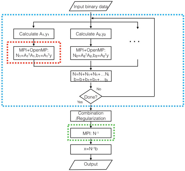
FIGURE 1. The parallel numerical calculation process by combining MPI and OpenMP in gravity field recovery.

In Figure 1, the blue dotted box indicates how to decompose the parallel computing process of design matrices and normal equation matrices. It uses the following independent property of observations, which shows how to divide them into n parts:

$\begin{array}{ll}\hfill A& ={\left[A_1{A}_2\dots A_n\right]}^T\hfill \\ \hfill N& =A^{T}A=\sum _{i=1}^n{A}_i^T{A}_i=\sum _{i=1}^n{N}_i\hfill \\ \hfill b& =A^{T}y=\sum _{i=1}^n{A}_i^T{y}_i=\sum _{i=1}^n{b}_i\hfill \end{array}(1)$

where A_i is a sub-block design matrix of A, N_i is a part of the normal matrix from the design matrix A_i, b_i is a part of the right side of the normal equation (sub-block matrix of b) which is the multiplication of the design matrix A_i and the observations of y_i (sub-block matrix of observations y). Here, we assume that the observations have equal weights and independent. In the gravity field recovery, e.g., IGGT_R1, the GOCE gravitational gradients were band-pass filtered, which could be used as independent, and the weights could be multiplied into the design matrix A_i (Lu et al., 2018b).

In the next step, we analyze how to use the MPI based on the partitioned solution as shown in Eq. 1. It means that column blocks of the design matrix are restored into certain processors, respectively. Here, each part of the normal equation matrix N_i (in the red dotted box in Figure 1) is designed to calculate in the same node to avoid data exchange between different nodes. The reason is to avoid using the Ethernet network between the different nodes mentioned above. Then multiplication of small blocks is calculated in each storage, as shown in Figure 2 (left). In this context, the multiplication results are restored in the corresponding storages, and the data is exchanged in storages, as shown in Figure 2 (right). After that, the corresponding values of matrix multiplication are calculated, and it continues to exchange data until the full values of matrix multiplication are completed. For this process, it is essentially presented in Figure 3 that the block diagonal matrices in the same color are calculated step by step after exchanging the data, e.g., the B₀ to B_p−1 are changed in sequence to each processors 0 to p − 1. Here, six kinds of color matrices represent the parallel calculation process for simplification. For example, Figure 2 (left) shows the result of black blocks in Figure 3 (left) at the very beginning while Figure 2 (right) indicates the result of brown blocks in Figure 3 (right) after first exchanging the B₀ to B_p−1 in each processors. In the actual calculation process, it only needs to calculate half of the normal equation matrix because of its symmetrical feature, such as the part of the red line triangle in Figure 3 (left). In order to simplify the computing program and combine the OpenMP in this calculation easily, the part of the red line box in Figure 3 (right) is actually calculated, which has almost no effect on calculation time compared to that red line box in Figure 3 (left). By taking the symmetrical feature of normal equations into account, it can reduce nearly half of the calculation to build normal equations, which costs most of the computing time in gravity field recovery.

FIGURE 2

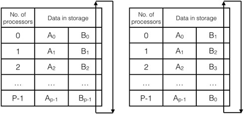
FIGURE 2. Data exchanging during the parallel calculation process of normal equations. A_i is a column block of the design matrix and B_i is the transpose of A_i. The left figure shows the data storage in the processors at the first step, while the right one shows the data storage exchange after finishing the first step in the loops.

FIGURE 3

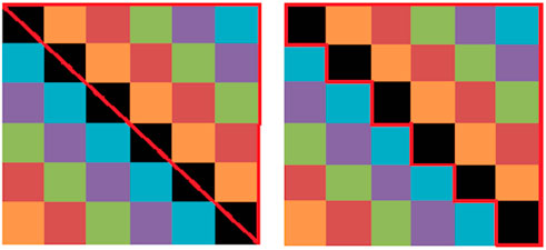
FIGURE 3. The parallel calculation process of matrix multiplication, six kinds of color matrices represent the parallel calculation process for simplifying. The left figure shows the block diagonal matrices in the same color are calculated step by step after exchanging the data in Figure 2. The right one shows that the part of the red line box is calculated based on the symmetrical feature of normal equations in gravity field recovery.

In MPI’s coarse-grained parallel circumstance, OpenMP’s fine-grained thread parallel programming models are implemented into the process in order to speed up the calculation progress further. This is mainly applied to the multiplication of small matrices in a single processor where exists nested loops. Therefore, it can increase the parallel granularity of the program by paralleling the outermost loop. In this context, the number of threads can be flexible according to cores on the single node to make full use of the CPUs and improve computational efficiency. On the other hand, the consumptions of the multiplications of small block matrices are reducing along with the loops of calculating block diagonal matrices as shown in Figure 3 (right). This is because of the symmetrical feature of normal equations as mentioned before. Therefore, the cores used in OpenMP thread parallel can be effectively allocated to the multiplication of the same color block diagonal matrices along with the loops.

As shown in Figure 1, each loop in the blue dotted box calculates the normal equation from a certain amount of satellite observations. The loop will end until all the input observations are completed in this calculation. Here, these main MPI and OpenMP functions were used as follows: MPI_COMM_GROUP accesses the group associated with given communicator which is used to control different groups to compute normal equation N_i as shown in the blue dotted box of Figure 1; MPI_COMM_CREATE creates new communicators corresponding to each group; MPI_SEND and MPI_RECV are used to exchange data when computing small blocks of normal equations as shown in Figure 3; OMP_SET_NUM_THREADS sets the number of threads in subsequent parallel regions which paralleling the outermost loop in multiplication of small blocks as mentioned above.

2.2 Inversion of normal equations

After obtaining the normal equation matrices using the parallel algorithm described before, we need to use the MPI to invert them in a parallel way which is shown in the green dotted line box of Figure 1. We use the Gauss-Jordan elimination method, which is suitable for inverting both symmetric and asymmetric matrices, and program it in FORTRAN language, where arrays are stored by column priority. The Gauss-Jordan elimination method with column exchange is used with a parallel algorithm, as described by previous studies (Melhem, 1987; Chen et al., 2004; Markus, 2012).

To implement the parallel calculation, we divide the columns of the matrix and use the main columns in a queue to perform elementary column transformations on the rest of the columns. Since the columns are independent in the inversion calculation, we divide the columns of the normal matrix to enable parallel computation while ensuring load balance between processors. As shown in Figure 4, assuming the number of processors is p, the order of the normal matrix is n, and the columns of the normal matrix i, i + p, … , i + (m − 1)p (same color columns in Figure 4) are restored in the processor of number i. Here, m = n/p. In the calculation, we point out the columns 0, 1, … , n − 1 as the primary columns in order and broadcast them to all processors. Each processor then takes turns choosing a primary column and broadcasts it to other processors. The processor that broadcasts the primary column applies this column to the remaining m − 1 columns as elementary column transformation, while the other processors perform elementary column transformation on m columns using the received primary column.

FIGURE 4

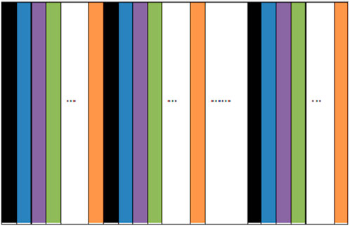
FIGURE 4. Cross classified storage of the normal matrix in the computer memory. Columns in the same color are stored in the corresponding processors. Each processor takes turns choosing a primary column and broadcasts it to other processors. The processor that broadcasts the primary column applies this column to the remaining m − 1 columns as elementary column transformation, while the other processors perform elementary column transformation on m columns using the received primary column. The loop continues until the last primary column with the number n − 1 is broadcast and the elementary column transformation is completed.

According to previous studies (Chen et al., 2004), p should be an exact divisor of n. However, we found that this is not a requirement and modified the program accordingly. If p is not an exact divisor of n, we set m to be the integer part of n/p plus one, and the values of some columns stored in certain processors are set to 0 if they are not allocated values from the normal matrix because (m + 1)*p > n. In addition, we set a judging condition to ensure that the program continues until the last primary column with the number n − 1 is broadcast and the elementary column transformation is completed. Otherwise, columns with the value 0 (n + 1, … , (m + 1)*p) will be broadcast, resulting in incorrect elementary column transformation.

In the calculation of inversion of normal equations, three main MPI functions were used: MPI_FILE_READ_AT and MPI_FILE_WRITE_AT are respectively used to read and write normal equations between hard disks and different processors by explicit offsets. MPI_BCAST broadcasts a message from the process with rank “root” to all other processes of the communicator. Here, it is used to broadcast the primary column in order to do the elementary column transformation.

3 Applications in gravity field recovery

To test the numerical algorithm as described above, we calculated an experimental version of the gravity field model IGGT_R1 (named IGGT_R1_test, degree/order 240) based on six synthetic gravitational gradients derived from the a priori gravity field model EIGEN-5C as a known value (Förste et al., 2008). The GOCE orbit positions are given in the Earth-fixed Reference Frame from the GOCE orbit product SST_PSO_2 (Gruber et al., 2010). The data period is from 01 November 2009, to 11 January 2010, as used in the first release of the European Space Agency’s (ESA) gravity field models based on GOCE observations (six million observations). Here, the methodology of gravity field modeling is based on the second invariant of the gravitational gradient tensor (Lu et al., 2018b). In processing the real data, the bandpass filtering is applied to the gravitational gradients. Therefore, the weight matrix (stochastic model) is a diagonal array derived from white noise. In this experimental study, the weight matrix is also a diagonal array and multiplied with the observation matrix before computing the normal equation matrix. The spectral behaviors of IGGT_R1_test are shown in Figure 5: The difference degree amplitudes for the testing model to the a priori model EIGEN-5C are at the level of 10^–16 to 10^–20. In contrast, they are at the level of 10^–12 to 10^–10 for the real gravity field models (e.g., GOCO01S and IGGT_R1C) to the reference model EGM 2008 (or EIGEN-6C4) which shows the accuracy level of current gravity field models (Pail et al., 2010; Pavlis et al., 2012; Lu et al., 2018a). It is even clearer from the coefficient differences between IGGT_R1_test and the priori model EIGEN-5C as shown in Figure 6. The coefficient differences are about −22 to −20 as absolute values in the logarithmic scale (log₁₀) except for the very low order parts and very high degree parts due to the influence of GOCE polar gaps. Here, the stand deviations of spherical harmonic coefficients from current gravity field models (e.g., EGM 2008, EIGEN-6C4) are at the level −12 to −10. Therefore, the calculation errors in this parallel numerical algorithm caused by the numerical accuracy of the current HPC cluster can be ignored.

FIGURE 5

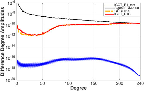
FIGURE 5. Difference degree amplitudes (unitless) of several gravity field models (GOCO01S and IGGT_R1C) w.r.t. EGM2008 and that of IGGT_R1_test w.r.t. its a priori model EIGEN-5C. The degree amplitudes of the EGM2008 model (black) are shown for reference.

FIGURE 6

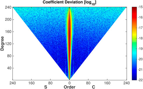
FIGURE 6. Coefficient differences between IGGT_R1_test and EIGEN-5C, provided as absolute values in logarithmic scale (log₁₀).

In addition, we also analyzed the calculating time and efficiency of the numerical algorithm. The calculation in this study was based on the HPC cluster in the School of Geodesy and Geomatics, Wuhan University. The MPI version used on the HPC cluster is MPICH-3.1b1 based on Intel Fortran. We used six nodes with 108 cores to compute and invert the normal equation of the testing model IGGT_R1_test as mentioned above. The calculation time of the normal equation was respectively 88, 40, and 27 h for the three different schemes as shown in Table 1. Here, the dimensions of A_i as shown in Figure 1 is 100 × 58077 in the calculation process. The first dimension was set as 100 by testing the calculation time between computing the blocks A_i and the corresponding multiplication ${A_i}^T{A}_i$. The second dimension is corresponding to the number (58077) of the spherical harmonic coefficients of the gravity field model (degree/order 240) in the simulation study. Here, the computation time of blocks ${A_i}_{(100\times 58977)}$ and ${y_i}_{(100)}$ was 0.8 h while the computation time of multiplication ${A_i}^T{A}_i$ was 25.8 h in the third scheme in Table 1. It shows that the numerical algorithm by combining MPI and OpenMP can improve the calculating efficiency, especially including consideration of the symmetrical feature of the normal equations. Apart from that, the calculating time will be linearly reduced as the computing resource increasing (e.g., more nodes). This is because of the independent property of design matrices and normal equation matrices as shown in Figure 1. On the other hand, the calculating time and relative efficiency to invert the normal equation matrix N_58077×58077 w.r.t. degree/order 240 are shown in Table 2. One thing that should be pointed out was that the calculating time in this table did not contain the input and output time to avoid the influence from other possible running programs due to the shared read and write resources of the HPC cluster. It is obvious that the calculating time is reducing as the number of processor cores increases. However, the communicating time is increasing between processors (also, between nodes) as the number of processor cores increases. Therefore, we use the computation time to divide the number of processor cores (H_i/100 × n_i) to define the relative efficiency of the inverting calculation. In this case, the smaller the numerical value is, the higher the relative efficiency is. We found that the relative efficiency generally decreases by using more processor cores in the inversion, especially when the number of processor cores is larger than 40. As the Gauss-Jordan elimination method does not make full use of the symmetrical feature to invert normal equation matrices, we further tested the Cholesky decomposition in our applications and hence installed the mathematical library ScaLAPACK on the HPC cluster. Here, two main functions from the mathematical library ScaLAPACK were used as follows: PDPOTRF computes the Cholesky decomposition while PDPOTRS solves a system of linear equations (Blackford et al., 1997). For example, the computation time is 0.16 h by using 100 processor cores to invert the normal equation matrix N_{58077 × 58077}. It is much faster compared to the MPI based Gauss-Jordan elimination method (1.76 h) due to the application of the symmetrical feature of the normal equation matrices and using level 3 BLAS which applies block-partitioned algorithms (e.g., Dongarra et al., 1990; Blackford et al., 2002; Goto and Van De Geijn, 2008). Here, the relative efficiency of Cholesky decomposition is 0.16, which is about ten times better than using the MPI-based Gauss-Jordan elimination method. Therefore, we suggested using the Cholesky decomposition if the matrices are symmetrical.

TABLE 1

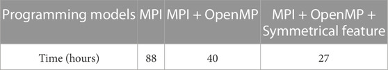
TABLE 1. The calculating time of computing the normal equation (N_{58077 × 58077}) by the parallel numerical algorithm. The calculation used six nodes with 108 cores from the HPC cluster in the School of Geodesy and Geomatics, Wuhan University.

TABLE 2

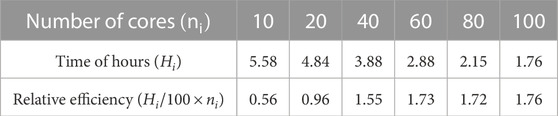
TABLE 2. The calculating time and relative efficiency of inverting the normal equation matrix (N_{58077 × 58077}) by the parallel numerical algorithm.

Furthermore, this parallel numerical algorithm was successfully applied to calculate the gravity field model named IGGT_R1 based on the real GOCE gravimetry data (Lu et al., 2018b). The numerical calculation progress was the same as the testing model IGGT_R1_test and its accuracy was at a similar level as ESA’s official released gravity field models with the same period of GOCE data (Pail et al., 2011). As far as we know, it was the first gravity field model calculated based on the invariants of the GOCE gravitational gradient tensor in a direct approach. Additionally, the parallel numerical algorithm was also applied to calculate the new gravity field model named IGGT_R1C which combines GOCE (IGGT_R1 (Lu et al., 2018b)), GRACE [ITSG-Grace2014s (Mayer-Gürr et al., 2014)], polar gravity anomalies [from the ArcGP project and PolarGap project (Forsberg and Kenyon, 2004; Forsberg et al., 2017)] and also Kaula’s rule of thumb (Kaula, 1966; Reigber, 1989) at the normal equation level to solve the GOCE polar gap problem (Lu et al., 2018a). In this combined model, the normal equation matrix N of GRACE comes from ITSG-Grace2014s and was gotten from its published variance-covariance matrix (Pavlis et al., 2012; Mayer-Gürr et al., 2014). For the GRACE model, we only used the part of the full normal equation matrix from d/o 2–150 and removed the shorter wavelengths to d/o 200 there by block matrix reduction:

$\left[\begin{array}{cc}\hfill N_{11}\hfill & \hfill N_{12}\hfill \\ \hfill N_{21}\hfill & \hfill N_{22}\hfill \end{array}\right]\left[\begin{array}{c}\hfill {\widehat{p}}_1\hfill \\ \hfill {\widehat{p}}_2\hfill \end{array}\right]=\left[\begin{array}{c}\hfill r_1\hfill \\ \hfill r_2\hfill \end{array}\right](2)$

where N₁₁, N₁₂, N₂₁, N₂₂ are blocks of the normal equation matrix of GRACE (N_GRACE), ${\widehat{p}}_1$, ${\widehat{p}}_2$ are blocks of the parameter vector $({\widehat{p}}_{\text{GRACE}})$ and r₁, r₂ are blocks of the right side of the normal equation of GRACE (r_GRACE). According to Eq. 2, the new normal equation i.e., the part of the full normal equation from d/o 2–150 of GRACE after the block matrix reduction is as follows:

$\left(N_{11}-N_{12}{N}_{22}^{-1}{N}_{21}\right)p_1=r_1-N_{12}{N}_{22}^{-1}{r}_2(3)$

Detailed methodologies and equations of the block matrix reduction can be found in previous studies (e.g., Schwintzer et al., 1991). This processing strategy was successfully applied to the GRACE normal equation matrices to infer the GOCE official gravity field models by the direct method (Bruinsma et al., 2010; Bruinsma et al., 2014) and EIGEN series [EIGEN-5C, Förste et al. (2008) and EIGEN-6C4, Förste et al. (2015)]. The reason for making this reduction was that the high-frequency gravity information (higher than d/o 150) from GRACE deteriorates due to striping errors. In this step of processing the GRACE normal equation matrix, the main numerical calculation was to invert the variance-covariance matrix to get the normal equation matrix and to invert part of the normal equation matrix for the block matrix reduction. In the next step, variance component estimation was applied to determine the weights of different types of observations efficiently (e.g., Förstner, 1979; Koch and Kusche, 2002). The main equation is as follows:

$\begin{array}{ll}\hfill N_c& =\sum _{i=1}^n{s}_{i,j}{N}_i\hfill \\ \hfill s_{i,j+1}& =\left(m_i-trace\left(N_c^{-1}{N}_i\right)\right)/v_i^T{P}_i{v}_i\hfill \\ \hfill s_{i,j}& =s_{i,j+1}\times s_{i,j}\hfill \end{array}(4)$

where N_i is the normal equation matrix of different types i, s_i,j is the weight of the corresponding normal equation, it is iteratively determined with the initial value set as 1, m_i is the number of observations, v_i and P_i represent the vectors of residuals and weighting matrix of different data types. From Eq. 4, the main numerical calculation occurs to invert the combined normal equation matrix N_c during the iterating numerical calculation of variance component estimation. We applied the numerical algorithm to the computations of gravity field recovery which represented above.

For further external checking and comparison with other global gravity field models, we checked IGGT_R1 and IGGT_R1C as well as some relevant gravity field models, e.g., GO_CONS_GCF_2_DIR_R1 (DIR-1) and GO_CONS_GCF_2_TIM_R1 (TIM-1), in GOCE orbit adjustment tests (Pail et al., 2011). The observations for the orbit tests are from GOCE kinematic 3D orbit positions (60 arcs from 1st November to 31st December of 2009) and the fit is calculated by dynamic orbit computation (e.g., Reigber, 1989; Dahle et al., 2012). Table 3 gives the RMS of the orbit fit residuals. From orbit adjustment tests, the accuracy of gravity field models based on GRAEC are improving due to the development of methodologies and increase of GRACE observations which is shown by comparing the RMS values of the orbit fit residuals from EGM 2008, EIGEN-5C, ITG-Grace2010s and ITSG-Grace2014s. Apart from that, GRACE-only models are better than GOCE-only models while combined models are better than single satellite models, e.g., comparing the RMS values of orbit fit residuals from ITG-Grace2010s, TIM-1 and GOCO01S. The IGGT_R1C is better than GOCO01S due to the contribution of more GRACE observations (ITSG-Grace2014s compared to ITG-Grace2010s) and the polar gravity anomalies (Mayer-Gürr et al., 2010; Pail et al., 2010). Additional GNSS/leveling checking and gravimetry data checking could be found in the former publications (Lu et al., 2018b; Lu et al., 2020).

TABLE 3

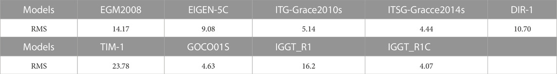
TABLE 3. External validation of gravity field models (d/o 180) by obit adjustment tests. RMS values of the orbit fit residuals (Unit: cm).

4 Potential geophysical applications

Satellite gravimetry data is helpful in studying the Earth’s structure and dynamics. For example, Llubes et al. (2003) studied the crustal thickness in Antarctica from CHAMP gravimetry which showed more detailed information about the crust than seismological models, especially in the western part of the continent. However, the gravity anomalies were reconstituted up to only degree 60 from the spherical harmonic coefficients, which means a very low spatial resolution of 333 km. After that, Block et al. (2009) researched regional crustal thickness variations under the Transantarctic Mountains and Gamburtsev Sub-glacial Mountains from the GRACE gravimetry. However, there were still unclear questions and debates over the Gamburtsev Subglacial Mountains’ origins due to the limitation of the GRACE gravimetry in terms of artifact striping, low spatial resolution, low accuracy at high degree parts (larger than 150), and so on. More recently, GOCE provided gravitational gradients with higher accuracy and spatial resolution, which helped to enhance our knowledge of the Earth’s structure and stress (e.g., Robert and Pavel, 2013; Eshagh, 2014; Sampietro et al., 2014; Ebbing et al., 2018; Llubes et al., 2018; Eshagh et al., 2020; Rossi et al., 2022). However, a polar data gap existed in the GOCE gravimetry due to the orbit inclination of 96.7°. In this context, our latest gravity field model IGGT_R1C combined GRACE and GOCE gravimetry as well as the latest airborne gravimetry data from the ESA’s PolarGap campaign (Forsberg and Kenyon, 2004; Forsberg et al., 2017). Therefore, it is potentially useful for geophysical and geological researching applications as mentioned above, e.g., estimating crustal thickness variations under the Transantarctic Mountains, which are in the GOCE polar data gap area and lack of airborne gravimetry data before the ESA’s PolarGap project. In addition, satellite gravimetry could be combined with air-marine gravimetry to study the local Earth’s structure, e.g., bathymetry beneath glaciers, determining the ocean bottom topography and so on (Lu et al., 2017a; Li et al., 2019a; Li et al., 2019b; Lu et al., 2019; Yang et al., 2020; Yang et al., 2021; Lu et al., 2022).

5 Discussion and conclusion

In this article, one parallel numerical algorithm was developed based on MPI and OpenMP to speed up the calculation progress of gravity field recovery. First, it combines MPI and OpenMP to compute the normal equations, which also considers its symmetrical feature to reduce the calculation time. Second, we modified the parallel Gauss-Jordan elimination method, which was used to invert normal equations. This modified software can be scaled up to 100 processor cores in the test during the calculation process, while only specific numbers of processors could be used in the traditional way regarding the Gauss-Jordan algorithm. In addition, we applied the Cholesky decomposition from the ScaLAPACK library in gravity field recovery and used it to compare with the parallel Gauss-Jordan elimination method. In this context, an experiment testing gravity field model named IGGT_R1_test was calculated based on six synthetic gravitational gradients from EIGEN-5C. The computation time to generate the normal equation of such a test model of degree/order 240 is 88, 44, and 27 h when applying the three different schemes (MPI, MPI and OpenMP, MPI and OpenMP including consideration of the symmetrical feature), respectively. The computation time to invert the normal equation is respectively 1.76 and 0.16 h by using the parallel Gauss-Jordan elimination method and the Cholesky decomposition from the ScaLAPACK library when 100 processor cores were used. Therefore, we suggested using the Cholesky decomposition from the ScaLAPACK library to invert symmetrical normal equation matrices in gravity field recovery. For non-symmetrical equation matrices, the parallel Gauss-Jordan elimination method could replace the Cholesky decomposition. From the numerical analysis, the calculation errors from the numerical algorithm can be ignored because the difference degree amplitudes for the testing model to the a priori model EIGEN-5C as a known value are at the level of 10^–16 to 10^–20 while they are at the level of 10^–12 to 10^–10 for the real gravity field models, which shows the accuracy level of current gravity field models. Furthermore, this numerical algorithm was successfully applied to calculate high-accuracy gravity field models (e.g., IGGT_R1, IGGT_R1C). External checking verifies these gravity field models based on the parallel numerical algorithm in this study are at a high accuracy level. Finally, high-accuracy gravity field models help improve our knowledge of the Earth’s structure and dynamics.

Data availability statement

Publicly available datasets were analyzed in this study. This data can be found here: https://earth.esa.int/eogateway/missions/goce/data.

Author contributions

Conceptualization, BL and ZL; Funding acquisition, ZL, BZ, and HZ; Methodology, BL and BZ; Software, BL, BZ, and HZ; Writing–original draft, BL; Writing–review and editing, ZL, BZ, and HZ.

Funding

This study was supported by the Chinese Scholarship Council (201506270158), the Fund of the Dutch Research Council (NWO) (ALWGO.2017.030), and the Natural Science Foundation of China (41704012, 41974015).

Acknowledgments

We would like to thank Mehdi Eshagh and an reviewer for taking the time and effort necessary to review the manuscript. We sincerely appreciate all valuable comments and suggestions, which helped us to improve the quality of the manuscript. We would like to express appreciation to Christoph Förste of GFZ for his kind help and discussions in GOCE orbit adjustment tests. Computing resources were provided by the high performance cluster of School of Geodesy and Geomatics, Wuhan University.

Conflict of interest

The authors declare that the research was conducted in the absence of any commercial or financial relationships that could be construed as a potential conflict of interest.

Publisher’s note

All claims expressed in this article are solely those of the authors and do not necessarily represent those of their affiliated organizations, or those of the publisher, the editors and the reviewers. Any product that may be evaluated in this article, or claim that may be made by its manufacturer, is not guaranteed or endorsed by the publisher.

References

Baur, O., Austen, G., and Kusche, J. (2008). Efficient GOCE satellite gravity field recovery based on least-squares using QR decomposition. J. Geodesy 82, 207–221. doi:10.1007/s00190-007-0171-z

CrossRef Full Text | Google Scholar

Baur, O. (2009). Tailored least-squares solvers implementation for high-performance gravity field research. Comput. Geosciences 35, 548–556. doi:10.1016/j.cageo.2008.09.004

CrossRef Full Text | Google Scholar

Blackford, L. S., Choi, J., Cleary, A., D’Azevedo, E., Demmel, J., Dhillon, I., et al. (1997). ScaLAPACK users’ guide. Philadelphia, Pennsylvania: SIAM.

Google Scholar

Blackford, L. S., Petitet, A., Pozo, R., Remington, K., Whaley, R. C., Demmel, J., et al. (2002). An updated set of basic linear algebra subprograms (BLAS). ACM Trans. Math. Softw. 28, 135–151.

Google Scholar

Block, A. E., Bell, R. E., and Studinger, M. (2009). Antarctic crustal thickness from satellite gravity: Implications for the transantarctic and Gamburtsev subglacial Mountains. Earth Planet. Sci. Lett. 288, 194–203. doi:10.1016/j.epsl.2009.09.022

CrossRef Full Text | Google Scholar

Brockmann, J. M., Roese-Koerner, L., and Schuh, W.-D. (2014a). A concept for the estimation of high-degree gravity field models in a high performance computing environment. Studia Geophys. Geod. 58, 571–594. doi:10.1007/s11200-013-1246-3

CrossRef Full Text | Google Scholar

Brockmann, J. M., Roese-Koerner, L., and Schuh, W.-D. (2014b). “Use of high performance computing for the rigorous estimation of very high degree spherical harmonic gravity field models,” in Gravity, geoid and height systems (Berlin, Germany: Springer), 27–33.

CrossRef Full Text | Google Scholar

Bruinsma, S. L., Förste, C., Abrikosov, O., Lemoine, J.-M., Marty, J.-C., Mulet, S., et al. (2014). ESA’s satellite-only gravity field model via the direct approach based on all GOCE data. Geophys. Res. Lett. 41, 7508–7514. doi:10.1002/2014gl062045

CrossRef Full Text | Google Scholar

Bruinsma, S., Marty, J., Balmino, G., Biancale, R., Foerste, C., Abrikosov, O., et al. (2010). “GOCE gravity field recovery by means of the direct numerical method,” in The 2010 ESA Living Planet Symposium, Bergen, Norway, 28 June - 2 July 2010. paper presented at the ESA Living Planet Symposium.

Google Scholar

Chandra, R. (2001). Parallel programming in OpenMP. Burlington, Massachusetts: Morgan kaufmann.

Google Scholar

Chapman, B., Jost, G., and Van Der Pas, R. (2008). Using OpenMP: Portable shared memory parallel programming, 10. Cambridge, Massachusetts: MIT press.

Google Scholar

Chen, G., An, H., Chen, L., Zheng, Q., and Shan, J. (2004). Parallel algorithm practice. Beijing: Higher Education Press. (in Chinese).

Google Scholar

Dahle, C., Flechtner, F., Gruber, C., König, D., König, R., Michalak, G., et al. (2012). GFZ GRACE level-2 processing standards document for level-2 product release 0005. Potsdam: GeoForschungsZentrum Potsdam, 20. Tech. Rep. - Data; 12/02. doi:10.2312/GFZ.b103-12020

CrossRef Full Text | Google Scholar

Dongarra, J. J., Cruz, J. D., Hammarling, S., and Duff, I. S. (1990). Algorithm 679: A set of level 3 basic linear algebra subprograms: Model implementation and test programs. ACM Trans. Math. Softw. (TOMS) 16, 18–28. doi:10.1145/77626.77627

CrossRef Full Text | Google Scholar

Drinkwater, M. R., Haagmans, R., Muzi, D., Popescu, A., Floberghagen, R., Kern, M., et al. (2006). “The GOCE gravity mission: ESA’s first core Earth explorer,” in Proceedings of the 3rd international GOCE user workshop (Pennsylvania: Citeseer), 6–8.

Google Scholar

Ebbing, J., Haas, P., Ferraccioli, F., Pappa, F., Szwillus, W., and Bouman, J. (2018). Earth tectonics as seen by GOCE-Enhanced satellite gravity gradient imaging. Sci. Rep. 8, 16356. doi:10.1038/s41598-018-34733-9

PubMed Abstract | CrossRef Full Text | Google Scholar

Eshagh, M., Fatolazadeh, F., and Tenzer, R. (2020). Lithospheric stress, strain and displacement changes from GRACE-FO time-variable gravity: Case study for sar-e-pol zahab earthquake 2018. Geophys. J. Int. 223, 379–397. doi:10.1093/gji/ggaa313

CrossRef Full Text | Google Scholar

Eshagh, M. (2014). From satellite gradiometry data to subcrustal stress due to mantle convection. Pure Appl. Geophys. 171, 2391–2406. doi:10.1007/s00024-014-0847-2

CrossRef Full Text | Google Scholar

Flechtner, F., Morton, P., Watkins, M., and Webb, F. (2014). “Status of the GRACE follow-on mission,” in Gravity, geoid and height systems (Berlin, Germany: Springer), 117–121.

CrossRef Full Text | Google Scholar

Forsberg, R., and Kenyon, K. (2004). “Gravity and geoid in the Arctic region—the northern polar gap now filled,” in Proceedings of 2nd GOCE User Workshop (Noordwijk: The Netherlands ESA Publication Division ESA SP-569).

Google Scholar

Forsberg, R., Olesen, A. V., Ferraccioli, F., Jordan, T., Corr, H., and Matsuoka, K. (2017). PolarGap 2015/16: Filling the GOCE polar gap in Antarctica and ASIRAS flight around South Pole. Retrieved from ftp://ftp.bas.ac.uk/tomj/PolarGAP/PolarGAP_radar_grids.zip.

Google Scholar

Förste, C., Bruinsma, S., Abrikosov, O., Lemoine, J., Marty, J., Flechtner, F., et al. (2015). EIGEN-6C4 the latest combined global gravity field model including GOCE data up to degree and order 2190 of GFZ Potsdam and GRGS Toulouse. Potsdam, Germany: GFZ Data Services. doi:10.5880/icgem.2015.1

CrossRef Full Text | Google Scholar

Förste, C., Flechtner, F., Schmidt, R., Stubenvoll, R., Rothacher, M., Kusche, J., et al. (2008). EIGEN-GL05C—a new global combined high-resolution GRACE-based gravity field model of the GFZ-GRGS cooperation. General Assembly European Geosciences Union (Vienna, Austria 2008). Geophys. Res. Abstr. 10. Abstract No. EGU2008-A-06944.

Google Scholar

Förstner, W. (1979). Ein Verfahren zur Schätzung von Varianz-Und Kovarianzkomponenten. Allg. Vermess. 86, 446–453.

Google Scholar

Goto, K., and Van De Geijn, R. (2008). High-performance implementation of the level-3 BLAS. ACM Trans. Math. Softw. 35, 1–14. doi:10.1145/1377603.1377607

CrossRef Full Text | Google Scholar

Gropp, W., Lusk, E., and Skjellum, A. (1999). Using MPI: Portable parallel programming with the message-passing interface, 1. Cambridge, Massachusetts: MIT press.

Google Scholar

Gruber, T., Rummel, R., Abrikosov, O., and van Hees, R. (2010). Tech. rep., GO-MA-HPF-GS-0110.GOCE level 2 product data handbook

Google Scholar

Kaula, W. M. (1966). Theory of satellite geodesy. Mineola, New York, United States: Dover Publications.

Google Scholar

Klees, R., Koop, R., Visser, P., and Van den Ijssel, J. (2000). Efficient gravity field recovery from GOCE gravity gradient observations. J. geodesy 74, 561–571. doi:10.1007/s001900000118

CrossRef Full Text | Google Scholar

Koch, K.-R., and Kusche, J. (2002). Regularization of geopotential determination from satellite data by variance components. J. Geodesy 76, 259–268. doi:10.1007/s00190-002-0245-x

CrossRef Full Text | Google Scholar

Li, M., Xu, T., Flechtner, F., Förste, C., Lu, B., and He, K. (2019a). Improving the performance of multi-GNSS (global navigation satellite system) ambiguity fixing for airborne kinematic positioning over Antarctica. Remote Sens. 11, 992. doi:10.3390/rs11080992

CrossRef Full Text | Google Scholar

Li, M., Xu, T., Lu, B., and He, K. (2019b). Multi-GNSS precise orbit positioning for airborne gravimetry over Antarctica. GPS solutions 23, 53–14. doi:10.1007/s10291-019-0848-9

CrossRef Full Text | Google Scholar

Llubes, M., Florsch, N., Legresy, B., Lemoine, J.-M., Loyer, S., Crossley, D., et al. (2003). Crustal thickness in Antarctica from CHAMP gravimetry. Earth Planet. Sci. Lett. 212, 103–117. doi:10.1016/s0012-821x(03)00245-0

CrossRef Full Text | Google Scholar

Llubes, M., Seoane, L., Bruinsma, S., and Rémy, F. (2018). Crustal thickness of Antarctica estimated using data from gravimetric satellites. Solid Earth. 9, 457–467. doi:10.5194/se-9-457-2018

CrossRef Full Text | Google Scholar

Lu, B., Barthelmes, F., Li, M., Förste, C., Ince, E. S., Petrovic, S., et al. (2019). Shipborne gravimetry in the baltic sea: Data processing strategies, crucial findings and preliminary geoid determination tests. J. Geodesy 93, 1059–1071. doi:10.1007/s00190-018-01225-7

CrossRef Full Text | Google Scholar

Lu, B., Barthelmes, F., Petrovic, S., Förste, C., Flechtner, F., Luo, Z., et al. (2017a). Airborne gravimetry of GEOHALO mission: Data processing and gravity field modeling. J. Geophys. Res. Solid Earth 122, 10,586–10,604. doi:10.1002/2017jb014425

CrossRef Full Text | Google Scholar

Lu, B., Förste, C., Barthelmes, F., Flechtner, F., Luo, Z., Zhong, B., et al. (2018a). Using real polar terrestrial gravimetry data to overcome the polar gap problem of GOCE - the gravity field model IGGT_R1C. Potsdam, Germany: GFZ Data Services. doi:10.5880/icgem.2019.001

CrossRef Full Text | Google Scholar

Lu, B., Förste, C., Barthelmes, F., Petrovic, S., Flechtner, F., Luo, Z., et al. (2020). Using real polar ground gravimetry data to solve the GOCE polar gap problem in satellite-only gravity field recovery. J. Geodesy 94, 34–12. doi:10.1007/s00190-020-01361-z

CrossRef Full Text | Google Scholar

Lu, B., Luo, Z., Zhong, B., Zhou, H., Flechtner, F., Förste, C., et al. (2017b). The gravity field model IGGT_R1 based on the second invariant of the GOCE gravitational gradient tensor. J. Geod. 92, 561–572. doi:10.1007/s00190-017-1089-8

CrossRef Full Text | Google Scholar

Lu, B., Luo, Z., Zhong, B., Zhou, H., Flechtner, F., Förste, C., et al. (2018b). The gravity field model IGGT_R1 based on the second invariant of the GOCE gravitational gradient tensor. J. Geodesy 92, 561–572. doi:10.1007/s00190-017-1089-8

CrossRef Full Text | Google Scholar

Lu, B., Xu, C., Li, J., Zhong, B., and van der Meijde, M. (2022). Marine gravimetry and its improvements to seafloor topography estimation in the southwestern coastal area of the baltic sea. Remote Sens. 14, 3921. doi:10.3390/rs14163921

CrossRef Full Text | Google Scholar

Markus, A. (2012). Modern fortran in practice. Cambridge, UK: Cambridge University Press.

Google Scholar

Mayer-Gürr, T., Eicker, A., Kurtenbach, E., and Ilk, K.-H. (2010). “ITG-GRACE: Global static and temporal gravity field models from GRACE data,” in System Earth via geodetic-geophysical space techniques (Berlin, Germany: Springer), 159–168.

Google Scholar

Mayer-Gürr, T., Zehentner, N., Klinger, B., and Kvas, A. (2014). “ITSG-Grace2014: A new GRACE gravity field release computed in Graz,” in Proceedings of GRACE Science Team Meeting (GSTM), Potsdam, 29, September–01, October, 2014. Available at: http://www.gfz-potsdam.de/en/section/global-geomonitoring-and-gravity-field/topics/development-operation-and-analysis-of-gravity-field-satellite-missions/grace/gstm/gstm-2014/proceedings/.

Google Scholar

Melhem, R. (1987). Parallel Gauss-Jordan elimination for the solution of dense linear systems. Parallel Comput. 4, 339–343. doi:10.1016/0167-8191(87)90031-7

CrossRef Full Text | Google Scholar

Migliaccio, F., Reguzzoni, M., and Sansò, F. (2004). Space-wise approach to satellite gravity field determination in the presence of coloured noise. J. Geodesy 78, 304–313. doi:10.1007/s00190-004-0396-z

CrossRef Full Text | Google Scholar

Pacheco, P. S. (1997). Parallel programming with MPI. Burlington, Massachusetts: Morgan Kaufmann.

Google Scholar

Pail, R., Goiginger, H., Schuh, W.-D., Höck, E., Brockmann, J., Fecher, T., et al. (2010). Combined satellite gravity field model GOCO01S derived from GOCE and GRACE. Geophys. Res. Lett. 37. doi:10.1029/2010gl044906

CrossRef Full Text | Google Scholar

Pail, R., Bruinsma, S., Migliaccio, F., Förste, C., Goiginger, H., Schuh, W.-D., et al. (2011). First GOCE gravity field models derived by three different approaches. J. Geodesy 85, 819–843. doi:10.1007/s00190-011-0467-x

CrossRef Full Text | Google Scholar

Pail, R., and Plank, G. (2002). Assessment of three numerical solution strategies for gravity field recovery from GOCE satellite gravity gradiometry implemented on a parallel platform. J. Geodesy 76, 462–474. doi:10.1007/s00190-002-0277-2

CrossRef Full Text | Google Scholar

Pavlis, N. K., Holmes, S. A., Kenyon, S. C., and Factor, J. K. (2012). The development and evaluation of the Earth gravitational model 2008 (EGM2008). J. Geophys. Res. Solid Earth 117. doi:10.1029/2011jb008916

CrossRef Full Text | Google Scholar

Reigber, C. (1989). “Gravity field recovery from satellite tracking data,” in Theory of satellite geodesy and gravity field determination (Berlin, Germany: Springer), 197–234.

Google Scholar

Reigber, C., Lühr, H., and Schwintzer, P. (2002). CHAMP mission status. Adv. space Res. 30, 129–134. doi:10.1016/s0273-1177(02)00276-4

CrossRef Full Text | Google Scholar

Robert, T., and Pavel, N. (2013). Effect of crustal density structures on GOCE gravity gradient observables. Terr. Atmos. Ocean. Sci. 24, 793–807. doi:10.3319/tao.2013.05.08.01(t)

CrossRef Full Text | Google Scholar

Rossi, L., Lu, B., Reguzzoni, M., Sampietro, D., Fadel, I., and van der Meijde, M. (2022). Global moho gravity inversion from GOCE data: Updates and convergence assessment of the GEMMA model algorithm. Remote Sens. 14, 5646. doi:10.3390/rs14225646

CrossRef Full Text | Google Scholar

Rummel, R., and Colombo, O. (1985). Gravity field determination from satellite gradiometry. Bull. géodésique 59, 233–246. doi:10.1007/bf02520329

CrossRef Full Text | Google Scholar

Rummel, R. (1993). “On the principles and prospects of gravity field determination by satellite methods,” in Geodesy and physics of the Earth (Berlin, Germany: Springer), 67–70.

CrossRef Full Text | Google Scholar

Sampietro, D., Reguzzoni, M., and Braitenberg, C. (2014). “The GOCE estimated moho beneath the Tibetan plateau and himalaya,” in Earth on the edge: Science for a sustainable planet (Berlin, Germany: Springer), 391–397.

CrossRef Full Text | Google Scholar

Schuh, W. D. (1996). Tailored numerical solution strategies for the global determination of the Earth’s gravity field. Mitteil Geod. Inst. TU Graz 81, 156.

Google Scholar

Schwintzer, P., Reigber, C., Massmann, F. H., Barth, W., Raimondo, J. C., Gerstl, M., et al. (1991). “A new Earth gravity field model in support of ERS-1 and SPOT-2: GRM4-S1/C1,” in Final report to the German Space Agency (DARA) and the French Space Agency (CNES). DGFI Munich/GRGS Toulouse 1991.

Google Scholar

Sneeuw, N. (2000). A semi-analytical approach to gravity field analysis from satellite observations. Ph.D. thesis. Technische Universität: München

Tapley, B. D., Bettadpur, S., Watkins, M., and Reigber, C. (2004). The gravity recovery and climate experiment: Mission overview and early results. Geophys. Res. Lett. 31. doi:10.1029/2004gl019920

CrossRef Full Text | Google Scholar

Yang, J., Guo, J., Greenbaum, J. S., Cui, X., Tu, L., Li, L., et al. (2021). Bathymetry beneath the Amery ice shelf, East Antarctica, revealed by airborne gravity. Geophys. Res. Lett. 48, e2021GL096215. doi:10.1029/2021gl096215

CrossRef Full Text | Google Scholar

Yang, J., Luo, Z., and Tu, L. (2020). Ocean access to Zachariæ Isstrøm glacier, northeast Greenland, revealed by OMG airborne gravity. J. Geophys. Res. Solid Earth 125, e2020JB020281.

CrossRef Full Text | Google Scholar

Yi, W. (2012). An alternative computation of a gravity field model from GOCE. Adv. Space Res. 50, 371–384. doi:10.1016/j.asr.2012.04.018

CrossRef Full Text | Google Scholar

Zhou, H., Luo, Z., Tangdamrongsub, N., Wang, L., He, L., Xu, C., et al. (2017a). Characterizing drought and flood events over the yangtze river basin using the hust-grace2016 solution and ancillary data. Remote Sens. 9, 1100. doi:10.3390/rs9111100

CrossRef Full Text | Google Scholar

Zhou, H., Luo, Z., Zhou, Z., Li, Q., Zhong, B., Lu, B., et al. (2018). Impact of different kinematic empirical parameters processing strategies on temporal gravity field model determination. J. Geophys. Res. Solid Earth 123, 10,252–10,276. doi:10.1029/2018jb015556

CrossRef Full Text | Google Scholar

Zhou, H., Luo, Z., Zhou, Z., Zhong, B., and Hsu, H. (2017b). HUST-Grace2016s: A new GRACE static gravity field model derived from a modified dynamic approach over a 13-year observation period. Adv. Space Res. 60, 597–611. doi:10.1016/j.asr.2017.04.026

CrossRef Full Text | Google Scholar