Uncertainty assessment of a permanent long-range terrestrial laser scanning system for the quantification of snow dynamics on Hintereisferner (Austria)

1 Introduction

Mass changes at the surface of a glacier dominate, in most cases, over internal and basal mass changes and form over a predefined period—usually the hydrological year or shorter—the so-called climatic glacier mass balance. It plays a crucial role in catchment hydrology and sea level rise. Furthermore, it is used to assess respective climate change impacts and is subjected to detection and attribution studies. In order to calibrate and validate high-resolution distributed glacier mass balance models, detailed information of glacier surface changes is needed (Klok and Oerlemans, 2002; Hock and Holmgren, 2005; Machguth et al., 2006).

The climatic mass balance information on the surface is often acquired with the traditional “direct glaciological method” (Kaser et al., 2003; Cuffey and Paterson, 2010; Cogley et al., 2011) by measuring the relative surface elevation changes at 10 to 50 selected locations (points) on the glacier. The measurements are transferred to mass changes in combination with density measurements of snow and ice and are then extrapolated to the glacier-wide surface. This “glaciological method” is laborious and resolves the complexity of spatial mass balance patterns only coarsely and is only grossly able to mirror the driving processes. On the contrary, the “geodetic method,” carried out from terrestrial or airborne platforms (Geist and Stotter, 2007; Fischer et al., 2016; Klug et al., 2018), allows for detecting comparatively high-resolution surface elevation changes relative to the surrounding bedrock. Again, obtained volume changes need measured, modeled, or assumed density information for conversion into mass changes. However, the geodetically measured glacier mass balance contains, beyond the climatic signal, the internal and basal changes in the ice column. In addition, it also contains effects of ice flow divergence, which is the elevation change component originating from the ice flux to maintain mass continuity (Cuffey and Paterson, 2010, Sect. 8.5.5). The ice flow divergence is omitted by integrating the elevation changes over the entire glacier area (Kuhn et al., 1999; Zemp et al., 2010; Klug et al., 2018). The effect of ice divergence on the point glacier mass balance may be neglected on glaciers with moderate to low ice flow dynamics and over short time periods such as daily up to monthly time intervals (Cuffey and Paterson, 2010). If, as on many mountain glaciers, internal and basal mass changes can also be neglected, the geodetically obtained mass changes can provide spatially and temporally distributed information on the climatic mass balance.

For most temperate and land-terminating glaciers, the representation of the snow cover dynamics poses the central deficiency in distributed mass balance models (Greuell and Bohm, 1998; Machguth et al., 2006; Carturan et al., 2012; Molg et al., 2012; Gurgiser et al., 2013; Ayala et al., 2015; Prinz et al., 2016). It crucially impacts the spatially distributed glacier surface mass balance by modulating accumulation and, subsequently, also ablation patterns. Data quantity and quality both from ground measurements and remote sensor systems have not yet been sufficient to reflect the actual snow cover processes on a glacier scale so far, which also limits the calibration and evaluation of distributed mass balance models (Machguth et al., 2006; Carturan et al., 2012; Gardner et al., 2013; Zemp et al., 2013).

A possible way to overcome this deficiency and acquire more information on surface elevation changes over the glacier is the measurement by a terrestrial laser scanner (TLS). A TLS emits a laser beam as the active sensing carrier. The distance between the sensor and the surface target is derived from the travel time of the laser beam and point clouds are created with a high point density ($>$1 points m⁻², depending on distance and scan settings) (Wehr and Lohr, 1999). Several studies have already proven that the total annual and seasonal mass balance can be acquired by TLS (Fischer et al., 2016; Wang et al., 2018; Xu et al., 2019). Since only the processes larger than the uncertainty of the TLS can be measured, an uncertainty assessment of the TLS is mandatory.

A permanent and automated TLS has been installed for monitoring the Hintereisferner (HEF) glacier (Ötztal Alps, Austria) in 2016. This TLS is able to capture 66.5% of the glacier area. Permanent TLS setups are known (Kromer et al., 2017; Vos et al., 2017; Anders et al., 2019; Deruyter et al., 2020; Campos et al., 2021) (Voordendag et al. (2021)), but not for studying glaciers and ranges longer than 2,500 m.

Various studies (Soudarissanane, 2016; Friedli, 2020) have already stated the main sources for uncertainty in TLS point cloud data: 1) instrument and hardware limitations, 2) scanning geometry, 3) atmospheric conditions between TLS and target surface, 4) surface reflectance properties, and 5) post-processing including registration and georeferencing. Additionally, the rasterization of point clouds contributes to the uncertainty budget when working with a digital elevation model (DEM). Previous research assessed only selected uncertainty sources and at shorter distance ranges than the system at HEF (Soudarissanane, 2016; Friedli, 2020; Kuschnerus et al., 2021; Dong et al., 2020; Schaer et al., 2007). Here, we addressed the full spectrum of the main uncertainty sources of TLS point clouds and derived DEMs and at distances up to 4,500 m.

This paper aims to:

1) identify and quantify the main sources of uncertainty for measuring surface changes with a permanent long-range TLS system and

2) assess the potential of the permanent long-range TLS system at HEF for detecting glaciologically relevant surface elevation changes.

The findings contribute to a better understanding of requirements and limitations of permanent TLS systems for observing glacier surface dynamics.

2 Study area

The research area is the HEF (Figure 1), a valley glacier located in the Rofental catchment in the Ötztal Alps (Austria). The glacier has a length of approximately 6,300 m, ranging between the Weißkugel mountain peak (3,739 m a.s.l., green triangle in Figure 1C) and the glacier tongue at 2,460 m a.s.l. (2018). The glacier has been the key research site of the University of Innsbruck for glaciological studies since the early days of glacier research (Blumcke and Hess, 1899) and is now a part of the wider Open Air Laboratory Rofental (Strasser et al., 2018). Continuous long-term mass balance observations dating back to the year 1952/53 (Kuhn et al., 1999) and velocity and ice thickness change measurements since 1895 (Span et al., 1997) are available. The glacier is classified as one of the key “reference glaciers” by the World Glacier Monitoring Service (WGMS) (Zemp et al., 2009).

FIGURE 1

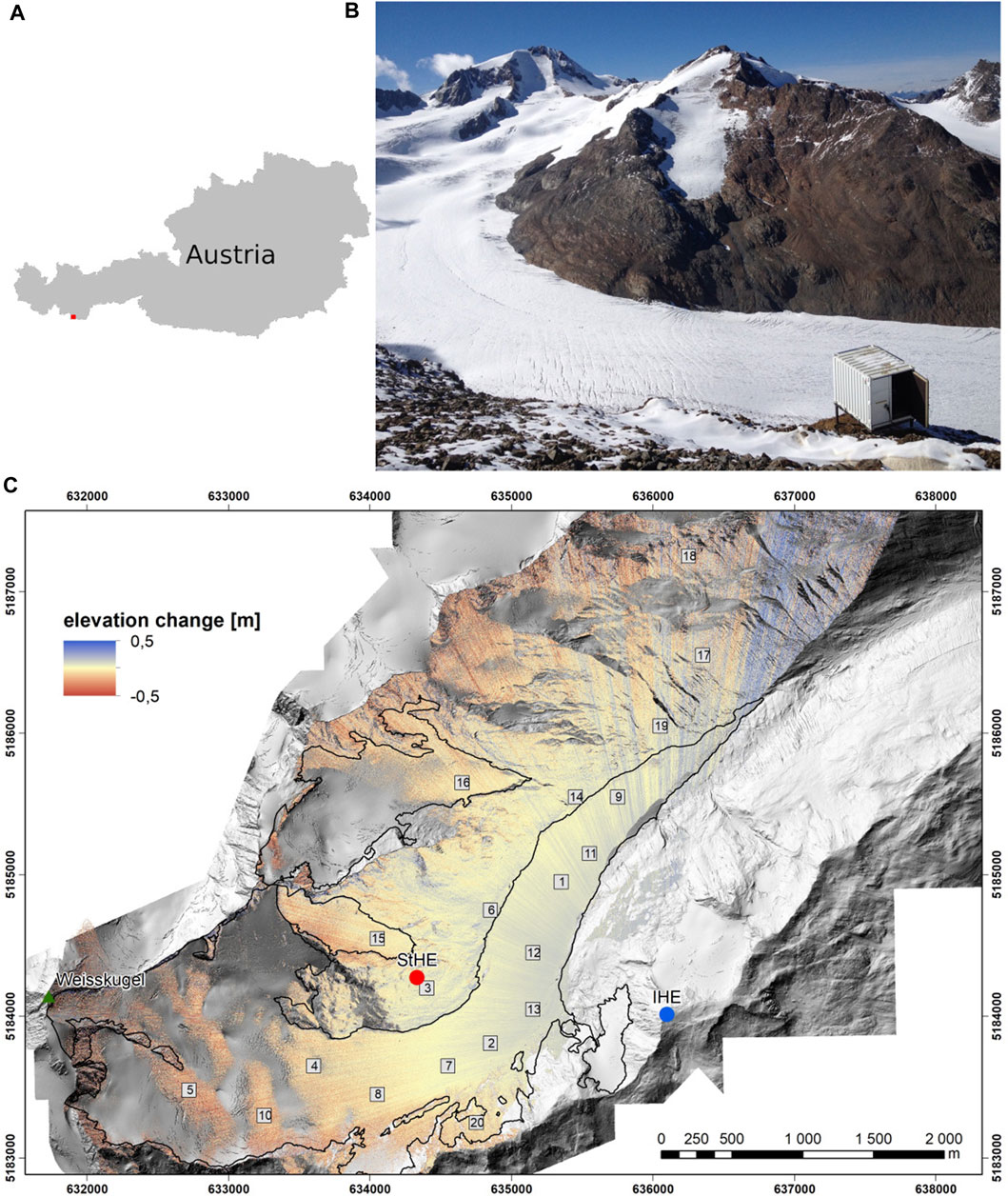
FIGURE 1. (A) Location of the Rofental (red square) in Austria. (B) TLS container overlooking HEF. Photo taken by Daniela Brugger, September 2016. (C) Differential plot after automated registration (Sect. 3.2) between 10:55 and 12:13 UTC on 5 November 2020. Twenty areas (boxes) of 100 by 100 m were selected at the glacier for detailed uncertainty analyses. The hillshade in the background and the glacier outlines are derived from the ALS data acquired by the Federal Government of Tyrol in 2018. IHE (3,245 m a.s.l.) is given as a blue dot, StHE (3,026 m a.s.l.) is the red dot, and the highest peak Weißkugel (3,739 m a.s.l.) is a green triangle.

The catchment is instrumented with several permanently operated and automated weather stations and rain gauges. The most important station for this study is Im Hinteren Eis (IHE, 3,245 m a.s.l.), which is located on the orographic right side of the glacier on the ridge at the Austrian–Italian border (blue dot in Figure 1C) and was installed in September 2016. The main instrument at this location is the year-round permanently installed TLS, which was installed in September 2016 and is in operational use for monitoring surface elevation changes on the glacier since 2019. The TLS is mounted on a stable frame positioned in a small container. The scanning process was automated in 2020, along with the setup, as described in detail by Voordendag et al. (2021). The TLS is a RIEGL VZ-6000 (RIEGL, 2019a), which can scan up to 6,000 m. Due to its laser wavelength of 1,064 nm, the instrument is exceptionally capable of measuring snow and ice. To date, the RIEGL VZ-6000 at HEF is the only permanent installation of such a long-range system worldwide, but we are also aware of the permanently installed RIEGL VZ-2000 TLSs (ranging up to 2000 m) at coast lines (Vos et al., 2017; Anders et al., 2019; Deruyter et al., 2020) and in a boreal forest (Campos et al., 2021).

Furthermore, Im Hinteren Eis is equipped with an automatic weather station (AWS), which is located 50 m horizontally and 25 m vertically away from the TLS. The AWS provides all common meteorological data at a 1-min resolution and also includes a 3D sonic anemometer to measure turbulent fluxes. Last, two webcams are installed that take pictures of the glacier every 30 min1.

A second important measurement location is Station Hintereis (StHE, 3,026 m a.s.l.), built in 1966 and located at the orographic left side of the glacier (Strasser et al., 2018). This station presently hosts an AWS with a 10-min average of common meteorological variables.

3 Analyses of five uncertainty sources

We are mainly interested in the uncertainty of the gridded data, as they ease the comparison of scans to identify vertical changes at the glacier. The measurements are subjected to six potential uncertainty sources (Table 1). However, this study does not account for the surface reflectance properties, as RIEGL VZ-6000 delivers good reflectance from snow and ice surfaces. As we are mainly interested in surface elevation changes during the season where the glacier is covered in snow, we assume a good reflectance and a negligible respective influence on surface elevation changes (Kaasalainen et al., 2008; Fritzmann et al., 2011). Thus, five uncertainty sources remain, and they will be discussed individually in this study. The uncertainty sources σ in this study are calculated as uncertainties in vertical direction of a single laser pulse or gridded data and are given in meter.

TABLE 1

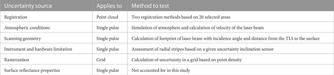
TABLE 1. Uncertainty sources relevant for the long-range TLS data, the element (single laser pulse, point cloud, or grid) they apply to, and the method of testing the magnitude of the uncertainty source.

The uncertainty that applies to a single-point measurement originates from the laser pulse source, the medium of the laser beam, and/or the target surface. The laser pulse source is the TLS, which has to deal with instrument and hardware limitations (Soudarissanane, 2016) (σ_instrument, Sect. 3.3). Atmospheric perturbations due to fluctuations and changes in air pressure, air temperature, and relative humidity along the path of the laser beam influence the velocity and pathway of the laser pulse in the medium (Friedli, 2020) and thus the calculated distance of a laser pulse (σ_atm, Sect. 3.4). The target surface is the footprint of the laser beam (Schaer et al., 2007; Sheng, 2008) and is elaborated as the scanning geometry in this study (σ_geo, Sect. 3.5). These three uncertainty sources are assumed to be random, independent uncertainties. The assumption of the independence of these uncertainty sources is a simplification, as they are all affected by the distance from the TLS to the surface R (800–4,500 m), which is several orders of magnitudes larger than these uncertainties (see Sect. 3.3–3.5). So, the influence of a small uncertainty in R, say R ± δR, is negligibly small on σ_instrument, σ_atm, and σ_geo, and R can be seen as an independent constant, which differs for every single laser pulse. After this simplification, the error propagation law for addition is applied in Eq. 1 to calculate the total error propagation of a single laser pulse.

${\sigma }_{\mathit{point}}=\sqrt{{\sigma }_{\mathit{instrument}}^2+{\sigma }_{\mathit{geo}}^2+{\sigma }_{\mathit{atm}}^2}(1)$

Subsequently, the acquired point clouds are gridded to DEMs by taking the mean of all the points in the 1-m grid cell. The number of points per grid cell is called the point density and decreases with the distance from the TLS. Likewise, if the point density increases, the uncertainty decreases, as the mean is taken over a higher number of points. The point density can be adjusted by changing the scan settings, but in our study, the angular step width of the TLS is set to 0.01° and not changed. The point density ρ_point can be seen as a repeated measurement and thus, due to the error propagation, the uncertainty of σ_point must be divided by the square-root of the number of measurements (Joerg et al., 2012) to get the uncertainty of every grid cell σ_gridcell (Eq. 2).

${\sigma }_{\mathit{gridcell}}=\frac{{\sigma }_{\mathit{point}}}{\sqrt{{\rho }_{\mathit{point}}}}(2)$

The calculated σ_gridcell does not yet include the uncertainty caused by the registration (see Sect. 3.2). The registration of the point clouds introduces a systematic error and is a rigid transformation and translation applied to the point clouds. Opposed to the other random uncertainty sources, the registration uncertainty depends on the method the user applies to the data, independent of the previously calculated σ_gridcell (Joerg et al., 2012; Fey and Wichmann, 2016). Therefore, the variable σ_reg is added to Eq. 2 to acquire Eq. 3.

${\sigma }_{\mathit{total}}=\frac{{\sigma }_{\mathit{point}}}{\sqrt{{\rho }_{\mathit{point}}}}+{\sigma }_{\mathit{reg}}(3)$

The registration uncertainty cannot be distinguished from the other uncertainty sources (Fey and Wichmann, 2016), and is therefore first assessed in Sect. 3.2.

3.1 Available data

For the uncertainty analyses, a period with stable surface conditions and as many TLS scans as possible are needed. Stable surface conditions are defined as a period where surface change due to snow drift or melt is unlikely to happen. Temperatures have to be low and the snow grains should already be well bonded throughout the snowpack. These conditions were met on 5 and 6 November, 2020, when the average temperature at IHE was −2.9 °C (at 1.5 m above ground), the average wind speed was 3.4 m s⁻¹ (at 3 m above ground), and no precipitation had been recorded since 27 October. The webcams did not give any evidence for blowing snow. Overall, 28 scans, taken between 5 November 10:55 UTC and 6 November 2020 15:05 UTC, were available. The scan taken on 5 November at 10:55 UTC is defined as the reference scan, as this is the first scan of the hourly TLS acquisitions.

3.2 Registration of scans

Acquired scans need to be registered in a common coordinate system and preferably also georeferenced in a global coordinate system. Previous publications employing a RIEGL VZ-6000 (Gabbud et al., 2015; Fischer et al., 2016; Xu et al., 2019) use RIEGL RiSCAN PRO software (RIEGL, 2019b) to manually register and georeference the scans. Unfortunately, this processing software cannot be implemented in an automated time series analysis. In order to overcome this limitation, to make longer time series analyses feasible and to test the effect of the registration method on the data, we designed an automated georeferencing tool chain in the System for Automated Geoscientific Analyses (SAGA GIS) (Conrad et al., 2015; Laserdata, 2022) based on an iterative closest point (ICP) algorithm (Besl and McKay, 1992), which we name ICP_HEF. In turn, the approach using RiSCAN PRO is called ICP_RiSCAN. For running ICP_HEF, a fix transformation matrix for the scanner’s orientation and position (SOP) is derived for a single selected scan using the RiSCAN PRO module multi-station adjustment (MSA) (Prokop and Panholzer, 2009; RIEGL, 2019b). All further scans are then adjusted with this fix transformation matrix. ICP_HEF assumes that the position of the TLS is stable, and thus, the same transformation matrix is applicable to all scans, whereas ICP_RiSCAN slightly changes the transformation matrix after manually applying the MSA algorithm. The advantage of ICP_HEF is that only one scan has to be registered manually to an existing project.

An alternative automated registration approach would be with the OPALS software (Pfeifer et al., 2014), where stable areas are selected at the surface of interest and a transformation matrix is based upon these stable areas. With this SOP matrix, the entire scan is referenced, but this approach is not possible at HEF, as most areas, except the walls of the research hut at StHE, get covered by snow. Another stable area is the mountain ridge in the direction of Weißkugel, but this is far away ($>$3,000 m) and, thus, barely reliable. Likewise, another possibility would be to install reflective targets, but this is not possible at HEF, as the footprints are large and thus large reflective targets are needed. These targets are also likely to get covered with snow or will move as they are not installed on a stable surface.

After registration and georeferencing, the point clouds are gridded to DEMs at 1 m resolution by taking the mean over all the points within a grid cell. A total of 20 areas surrounding and on the glacier are selected for the comparison between scans (Figure 1C). The selected areas cover 100 by 100 m and contain 10,000 pixels each. The differences between the 28 scans and the reference scan are calculated, and the average difference of the areas relative to the reference scan are calculated and reported. This is done for both the registration methods with ICP_RiSCAN and ICP_HEF, respectively.

The mean differences relative to the reference scan of the 100 by 100 m areas with ICP_RiSCAN are shown in Figure 2A. They range between −0.15 and +0.04 m in a vertical direction, even though zero change was expected. The largest deviations relative to the reference scan (red encircled in Figure 2) are found for the areas furthest away from the TLS, whereas the closer areas (yellow to orange colors in Figure 2A) have deviations closer to 0.0 m.

FIGURE 2

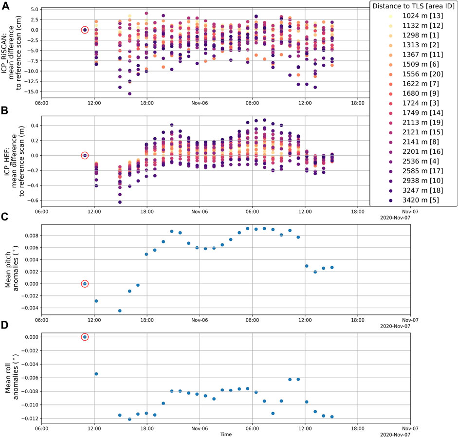
FIGURE 2. Mean difference of 20 selected areas relative to the reference scan of 5 November 10:55 (red encircled) with (A) ICP_RiSCAN (in cm) and (B) ICP_HEF (in m). Mean (C) pitch and (D) roll as measured by the internal inclination sensors. The legends in (A) and (B) correspond to the areas in Figure 1C, sorted to the distance from IHE. Please note the different orders of magnitude of the different registration methods in (A) and (B).

ICP_HEF shows different results, as the deviations range between −0.62 m and +0.47 m (Figure 2B). The deviations relative to the reference scan increase if the distance from the selected area to the TLS is increasing, so the deviations can strongly be assigned to the scanning distance. The changes observed in Figure 2B are compared to the measurements of the internal inclination sensors of the TLS. The mean roll and pitch of every scan has been calculated (Figure 2C, D), and the pitch anomaly of the scans shows a similar pattern as the mean differences in Figure 2A. This shows that the assumption that the position of the TLS is stable during consecutive scans is not valid because the TLS moves slightly.

Taking a closer look at single scans with ICP_RiSCAN (Figure 2A), it can be seen that the differences between the 20 areas range between 0.06 m (on 6 November at 4:30 UTC) and 0.19 m (on 5 November at 16:01 UTC). The smallest ranges of difference between the 20 areas are found at night, which might indicate differences caused by the atmospheric conditions or incoming solar radiation. The deviations have been compared to air temperature and wind data from the nearby AWS IHE. The temperature data showed an increase of approximately 4 °C after 6 November, 6:00 UTC, but no correlation with the deviations in Figure 2A was found. Similarly, higher wind speed in the night between 5 and 6 November and a peak in the turbulence kinetic energy on 6 November at around 3:00 UTC did not show correlation with the deviations relative to the reference scan.

It can be concluded that the average vertical accuracy of the TLS data at grids of 100 m is ±0.10 m for scans registered and georeferenced with ICP_RiSCAN and ±0.50 m for ICP_HEF. The accuracy strongly depends on both the distance from the TLS to the surface and the applied registration method. However, the absolute magnitude of the registration uncertainty σ_reg remains elusive as, in addition to the remaining registration uncertainty, the other uncertainty sources are also included in this calculation.

3.3 Instrument and hardware limitations

Preliminary results applying ICP_HEF show stripes which extend radially from the position of the TLS to the surface in the DEMs, particularly visible in difference plots between two DEMs, i.e., at the glacier tongue, around areas 17–19, in Figure 1C. The magnitude of the stripes in the vertical direction is about ±0.10 m in a difference plot (Figure 1C).

The radial stripes are possibly caused by wind, turbulence, and thermal changes of the mounting platform of the TLS during data acquisition (Kuschnerus et al., 2021; Voordendag et al., 2021). The exact source is not investigated in this study, as accurate measurements of wind, temperature, and turbulence were unavailable at the exact location of the TLS and, thus, the radial stripes are only investigated with the data of the internal inclination sensors. It is hypothesized that these stripes are caused by movements of the TLS at high frequencies. The internal inclination sensors measure at 1 Hz and have an accuracy of ±0.008°. The TLS measures the time-of-flight of a laser pulse and calculates the distance from the TLS to the surface with it. The position of this laser pulse is calculated with the beam direction and beam origin. The beam direction and origin of the laser pulse should be adjusted by using the measurements of the internal inclination sensors, if the TLS moves. The x-, y-, and z-coordinates in the Scanner’s Own Coordinate System (SOCS) are called vertices in RIEGL’s RiVLib (Eq. 4, where i denotes x, y, or z) (RIEGL, 2013).

$vertex\left[i\right]=beam\text{\_}origin\left[i\right]+echo\text{\_}range\cdot beam\text{\_}direction\left[i\right](4)$

Regardless of the adjustments made in the beam direction and origin, an uncertainty attributed to the radial stripes σ_instrument remains for every single laser pulse. It is assumed that this depends on the distance R and the uncertainty of the internal inclination sensor as given by the manufacturer of ±0.008° (Eq. 5). We consider these radial stripes as the total uncertainty attributed to the instrument and hardware limitations.

${\sigma }_{\mathit{instrument}}=R\cdot \sin \left(0.008°\right)(5)$

Figures 3A, B show the measurements by the inclination sensors in roll (x) and pitch (y) of the reference scan, respectively. The variation in the inclination data indicates high-frequency vibrations. The TLS at IHE is installed slightly tilted to adjust its field-of-view downward to the glacier. A sinusoid is plotted through the inclination data with a least-squares method (Figures 3A, B).

FIGURE 3

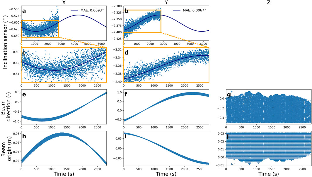
FIGURE 3. (A) Roll measurement with its calculated trend through the data, (B) pitch measurement with its calculated trend through the data, (C, D) zoomed area of the orange boxes in (A, B), respectively, (E–G) beam direction, and (H–J) beam origin as read from the raw data sampled at every 1000th point. The mean absolute error (MAE) of the trend through the roll and pitch data is given in (A, B).

The shapes of the curves of the beam direction (Figures 3E, G) and beam origin (Figures 3H, I) in the x- and y-directions depend on the rotation of the TLS around its tilted z-axis (Lichti and Shaloud, 2010). The beam direction and origin in the z-direction (Figures 3G, I) depend on the rotation of the mirror in the TLS and show the relief of the mountain ridge. Although the measured inclination data of the reference scan is noisy, Figures 3E, F show a rather smooth beam direction. The frequency of the inclination data is 1 Hz, and these data are not used to correct individual scan lines, but a mean value is calculated from the data [B. Groiss (Riegl), personal communication, 29 October 2020]. This value is used to level the instrument by means of an SOP matrix and shows the good correspondence between the inclination data and beam direction. This means that small movements in the scanner are not corrected in the individual scan lines and, thus, the individual scan lines show deviations in the form of radial stripes. These deviations become especially apparent if the difference between two DEMs with a grid cell size of 1 m is calculated.

Theoretically, it would be possible to correct the beam direction with the inclination measurement, but this is not feasible as the effective measurement rate of the TLS is 23,000 measurements per second (pulse repetition rate of 30 kHz) and the frequency of the inclination data is only 1 Hz. In addition, the starting time of the inclination sensors cannot directly be coupled with the start of the TLS measurement, as an approximate 5-second difference is found between the total scanning time and the number of inclination measurements.

The uncertainty related to the instrument and hardware limitations σ_instrument, according to Eq. 5, is found between 0.09 and 0.64 m and only depends on the distance from the TLS to the surface (Figure 4).

FIGURE 4

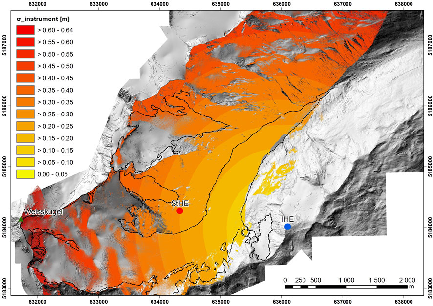
FIGURE 4. Distributed TLS uncertainty related to instrument and hardware limitations (σ_instrument).

3.4 Influence of atmospheric conditions on the laser beam

The distance R of a laser pulse is measured with the time-of-flight of a laser beam to the surface τ and the velocity of the laser beam in the propagating medium c_g (Eq. 6) (RIEGL, 2019b).

$R=c_g\frac{\tau }{2}=\frac{c_0}{n_g}\frac{\tau }{2}(6)$

The laser beam is delayed by the group index of refraction n_g relative to the speed of light in vacuum c₀. n_g depends on the group refractivity N_g at 0°C, 1,013.25 hPa, and 0% relative humidity (RH) and the wavelength λ (1.064 μm) (Eq. 7) (RIEGL, 2019b). The group refractivity N_L at ambient moist air at temperature T (°C), pressure p (hPa), and vapor pressure e is calculated with Eq. 8 (RIEGL, 2019b), and this leads to the group index of refraction (Eq. 9) (RIEGL, 2019b).

$N_g=287.6155+\frac{4.88660}{{\lambda }^2}+\frac{0.06800}{{\lambda }^4}(7)$

$N_L=\frac{273.15}{1013.25}\frac{N_{g}p}{T+273.15}-\frac{11.27e}{T+273.15}(8)$

$n_g=1+N_L\cdot 10^{-6}(9)$

The RIEGL VZ-6000 is able to correct for n_g, but assumes constant temperature, pressure, and humidity along the path of the laser beam. This assumption is not valid in mountainous terrain at long ranges as air temperature and air pressure differ widely over this terrain.

The atmospheric influence on the laser beam can only be assessed with spatio-temporal information at high-resolution of the relevant atmospheric variables (air temperature, RH, and air pressure) along the laser beam path. However, three-dimensional observations of the atmosphere over the glacier are not available. To overcome this data gap, numerical simulations with the Weather Research and Forecasting (WRF) model are performed over HEF and surroundings. A detailed model evaluation study (Goger et al., 2022) within a measurement campaign over the glacier (Mott et al., 2020) has shown that the WRF model is able to simulate the general atmospheric boundary layer structure over HEF successfully. The same high-resolution large-eddy simulation (LES) setup is used with a horizontal grid spacing of Δx = 48 m for 5 and 6 November, 2020. The model output is used as three-dimensional, realistic information of atmospheric variables above the glacier. A path along the laser beam through the atmosphere is interpolated at increments of approximately 13 m. It is assumed that the last 10 m of the laser beam travels through the glacier boundary layer. The temperature in these last 10 m is linearly interpolated between the simulated temperature at 2 m and the simulated surface temperature. The simulation of the air temperature, RH, and air pressure is compared against the observations, similar to Goger et al. (2022) and enables the calculation of the changing n_g along the laser beam path.

The difference in path length ΔR relative to the entire distance R is consequently calculated with Eq. 10 (Friedli, 2020) and the refractive index according to the instrument settings at IHE n₀ (RIEGL, 2019b), where the temperature is permanently set to −2°C, pressure to 684 hPa, and the RH to 28%.

$\mathrm{\Delta }R={\int }_0^R\left(n_0-n_g\left(s\right)\right)ds(10)$

The laser beam is also refracted due to the changing n_g. The angle of refraction γ is calculated with the derivative of the refractive index perpendicular to the path $\frac{dn(s)}{dq}$ (Eq. 11) (Friedli, 2020). It is decided not to simulate the refraction of the laser beam in our study, as the derivative of the refractive index perpendicular to the path is needed, and this is not accurate in our high-resolution simulation with a horizontal grid spacing of Δx = 48 m.

$\gamma ={\int }_0^R\frac{R-s}{R}\frac{dn\left(s\right)}{dq}ds(11)$

The calculated change of the laser beam distance is not yet the vertical component of the uncertainty caused by the atmospheric conditions. The vertical component of the uncertainty as attributed to atmospheric effects σ_atm is calculated with slope γ and incidence angle θ in Eq. 12 and clarified with Figure 5A.

${\sigma }_{\mathit{atm}}=\mathrm{\Delta }R\cdot \frac{\cos \theta }{\cos \gamma }(12)$

FIGURE 5

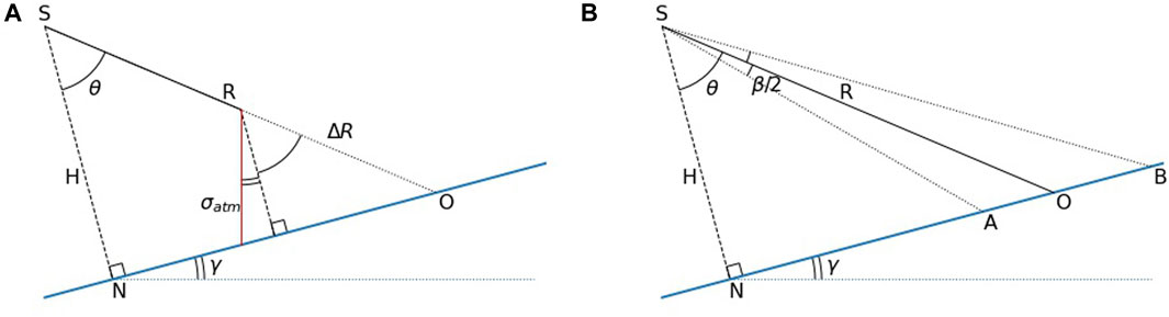
FIGURE 5. Geometry of the laser beam from the TLS at S to a point at the surface O with distance R. The blue line is a plane through O with H being a normal on this plane. (A) Change in the distance of the laser beam from S to O, ΔR, is calculated from the LES (Sect. 3.4). The extent of σ_atm is calculated with slope γ and incidence angle θ. (B) AB is the major axis of the elliptical footprint, θ the incidence angle, and β the beam divergence.

Figure 6 shows a cross-section of the simulated air temperature for area 4 on 5 November at 12:00 UTC, and 6 November 00:00 and 07:00 UTC. This shows the high variability of the air temperature over space and time. The green star indicates the position of the TLS and the green line indicates the laser beam path in the simulation. The position of the TLS and the length of the laser beam path in the simulation slightly differ from the reality (Table 2) because the model uses a coarser topography than that measured with the TLS (Figure 6). The simulated data show a decrease in the length of the laser beam between −0.0029 and 0.0194 m (Figure 7). The anomalies increase with increasing distances but are relatively small compared to the uncertainty caused by the instrument and hardware limitations and, as we will later see, the scanning geometry. However, temperatures having the largest influence on the velocity of the laser beam through the atmosphere (Friedli, 2020) were close to the default temperature of −2.0°C of the TLS at 5 and 6 November (−2.9°C on average).

FIGURE 6

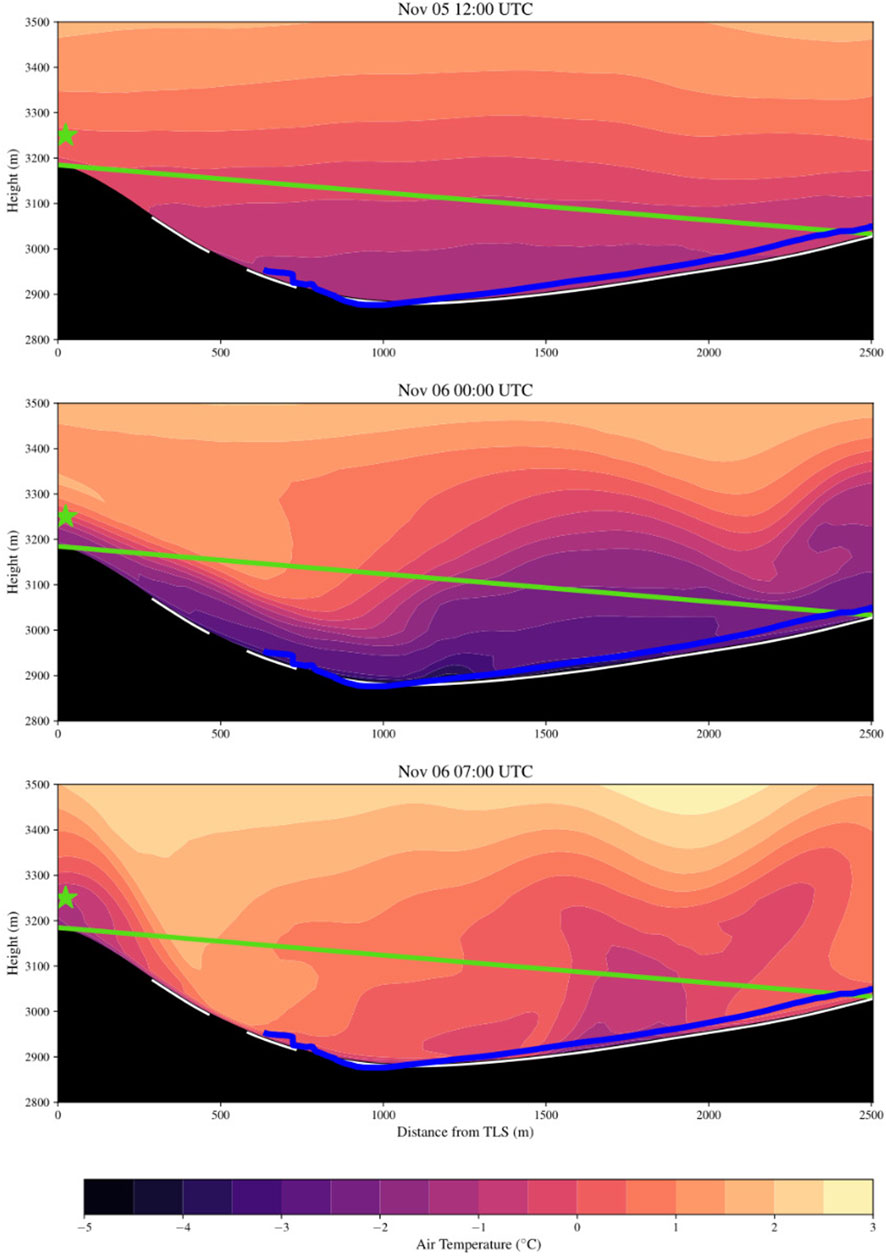
FIGURE 6. Temperature plot for the cross-section from TLS to area 4 for 5 November 12:00 UTC, and 6 November 00:00 and 07:00 UTC. The black area is the topography as used in the simulation, with white areas indicated as the glacier area. The blue line is the topography as measured with the TLS. The green line is the laser beam in the simulation and the green star is the position of the TLS in reality.

TABLE 2

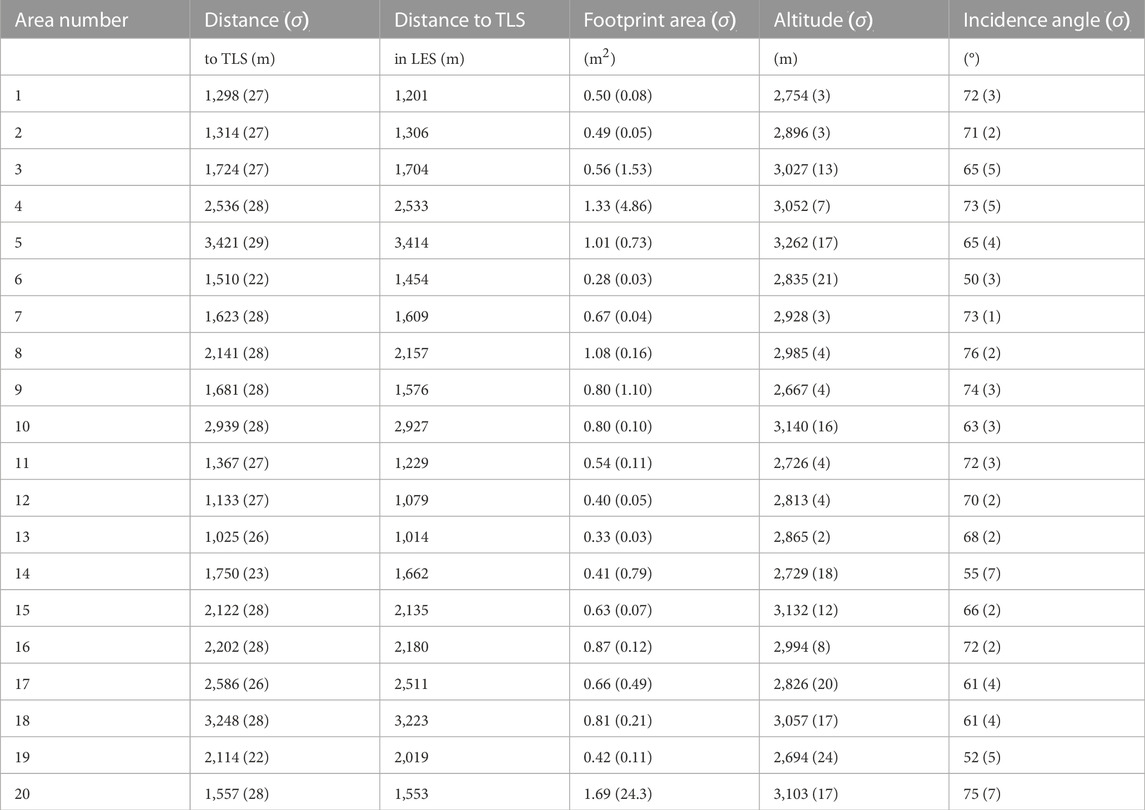
TABLE 2. Mean distance to the TLS as measured by the TLS and as used in the LES, mean footprint areas, mean altitude above the sea level, and mean incidence angle with standard deviations σ of the areas denoted in Figure 1.

FIGURE 7

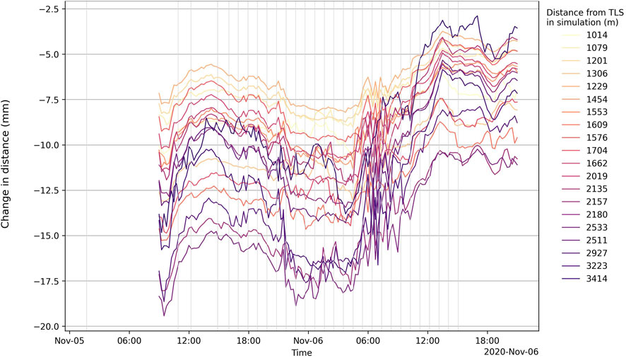
FIGURE 7. Change in the distance traveled by the laser beam in mm for 20 different areas over time (Y-axis). The legend shows the distance of the TLS to the simulated coordinates. The vertical gray lines denote the time a new scan was started. The temporal resolution of LES simulation is 15 min.

Therefore, the change in the laser beam distance with a temperature increase and decrease of 10°C was also calculated. This shows changes in distance as low as −0.0424 m (−10°C) and as high as +0.0210 m (+10°C), respectively. A similar sensitivity study was performed for RH (±25%) and air pressure (±10 mbar). The simulated air pressure only varies with the altitude and is relatively constant over time. The simulated relative humidity varies more, but uncertainties due to variations in the relative humidity are so small that they can be neglected (Friedli, 2020). Thus, changes in air pressure and RH have no significant influence on the change of distance measurements.

3.5 Scanning geometry

This section deals with the incidence angle and the consequent footprint of the laser beam on the target surface to quantify the contribution of the scanning geometry. The shorter the distance and the closer the incidence angle to the normal, the smaller the respective uncertainty and vice versa (Soudarissanane, 2016).

The footprint of the laser beam is an ellipse under the assumption that the illuminated surface is a plane, and the laser beam is not perpendicular to this plane. The incidence angle θ to the surface has been calculated with the terrain normal n and the laser beam direction l in Eq. 13 (Schaer et al., 2007).

$\theta =\arccos \left(\frac{l\cdot n}{|l\Vert n|}\right)(13)$

A normal of the terrain was calculated with the slope (γ) and aspect (α) (Zevenbergen and Thorne, 1987) from the DEMs and Eq. 14.

$\left(\begin{array}{c}\hfill n_1\hfill \\ \hfill n_2\hfill \\ \hfill n_3\hfill \end{array}\right)=\left(\begin{array}{c}\hfill \sin \alpha \sin \gamma \hfill \\ \hfill \cos \alpha \sin \gamma \hfill \\ \hfill \cos \gamma \hfill \end{array}\right)(14)$

The extent of the major axis M of this ellipse depends on the incidence angle with the surface from the TLS, the distance R, and the beam divergence β of the laser pulse. The extent of the minor axis m of the ellipse only depends on the distance and beam divergence. The beam divergence β of the RIEGL VZ-6000 is 0.12 mrad (RIEGL, 2019a). The major axis of the footprint is derived using Eq. 15 (Sheng, 2008), where H, OA, and OB comprise the geometry from Figure 5B; the extent of the minor axis is derived using Eq. 16 (Sheng, 2008).

$\begin{array}{ll}\hfill M=OA+OB& =H\cdot \left[\tan \left(\theta +\beta /2\right)-\tan \left(\theta -\beta /2\right)\right]\hfill \\ \hfill & =2R\cos \theta \cdot \frac{\sin \beta }{\cos 2\theta +\cos \beta }\hfill \end{array}(15)$

$m=2H\cdot \frac{\tan \beta /2}{\cos \theta }=2R\cos \theta \cdot \frac{\sin \beta }{\cos \theta \left(1+\cos \beta \right)}=2R\cdot \frac{\sin \beta }{1+\cos \beta }(16)$

Last, the footprint area A_F, which is the illuminated spot on a planar surface from the laser beam, is calculated with Eq. 17.

$A_F=\pi \cdot M\cdot m(17)$

To calculate the contribution of the scanning geometry to the entire uncertainty budget, the major axis is decomposed in x-, y-, and z-components. The z-component is the main interest, as we are interested in vertical changes over the glacier. The vertical component is approximately 1/3 of the vertical component of the major axis M_Z (Schaer et al., 2007). We define this extent as the vertical uncertainty caused by the scanning geometry σ_geo (Eq. 18).

${\sigma }_{\mathit{geo}}=M_Z/3(18)$

The distance measured by the TLS and as used in the LES (Sect. 3.4), the footprint area, mean altitude above the sea level, and incidence angle for the boxed areas from Figure 1C are given in Table 2. The total footprint area (Eq. 17), which is the illuminated spot on the planar surface, increases up to an area of 1.33 m². Area 20 has a very large σ for the footprint, which is caused by the incomplete coverage of the 100 by 100 m area and the high incidence angle, and thus, it is assumed to be an outlier in the dataset.

After the decomposition of the x-, y-, and z-components and Eq. 18, the contribution of the scanning geometry in the uncertainty budget is approximated between 0.02 and 0.25 m (Figure 8) in the vertical direction for a grid size of 1 m. σ_geo is between 0.20 and 0.25 m close to Weißkugel and 0.02 and 0.05 m in the area between IHE and StHE.

FIGURE 8

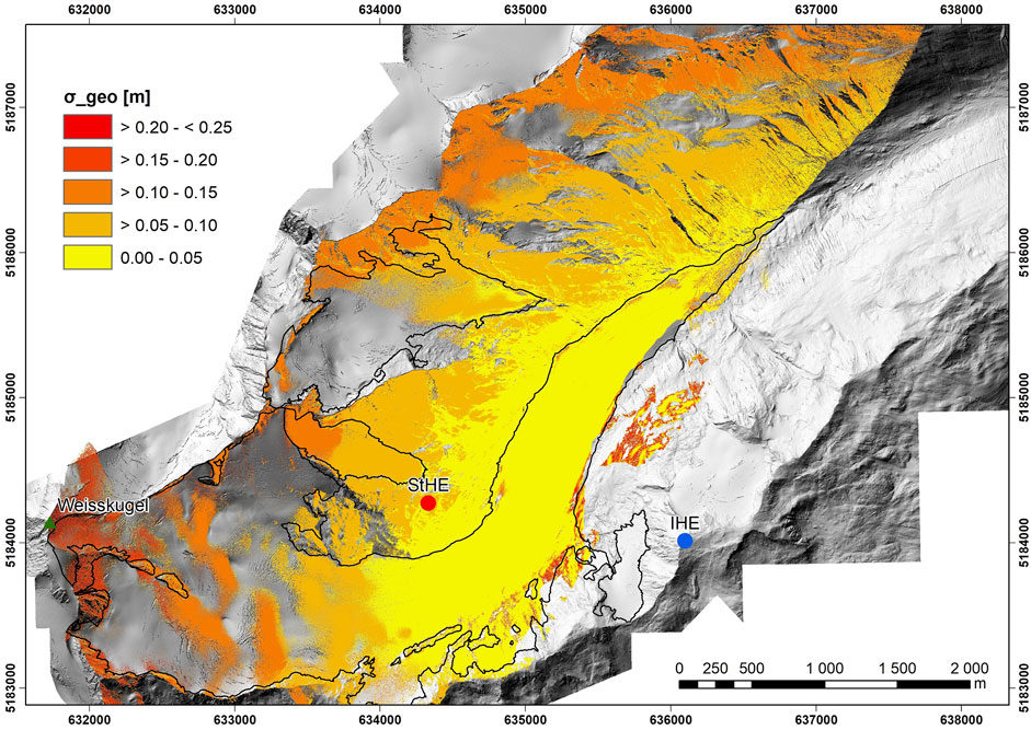
FIGURE 8. Distributed TLS uncertainty related to the scanning geometry (σ_geo).

3.6 Rasterization

In the previous three sections, all uncertainty sources that apply to a single pulse are described. These uncertainty sources are now combined to form the total uncertainty σ_gridcell, without accounting for the registration uncertainty. The uncertainty of a single laser pulse is found in Figure 9. As the uncertainty depending on the influence of the atmosphere on the laser beam over time is highly variable and depends on the distance from the TLS, we have taken a value of 0.01 m for σ_atm in Eq. 1 as this is approximately the average of the change in distance from Figure 7. Furthermore, σ_atm is an order of magnitude smaller than σ_instrument and σ_geo, and so, the influence of the atmosphere is relatively small. The uncertainty of a single laser pulse ranges between 0.09 m at the area closest to the TLS and 0.66 m in the accumulation zone close to Weißkugel. These values are close to the values found in Sect. 3.3 and show that σ_instrument is the largest contributor to the uncertainty budget. Furthermore, all three uncertainty sources (σ_instrument, σ_geo, and σ_atm) strongly depend on distance R from the TLS.

FIGURE 9

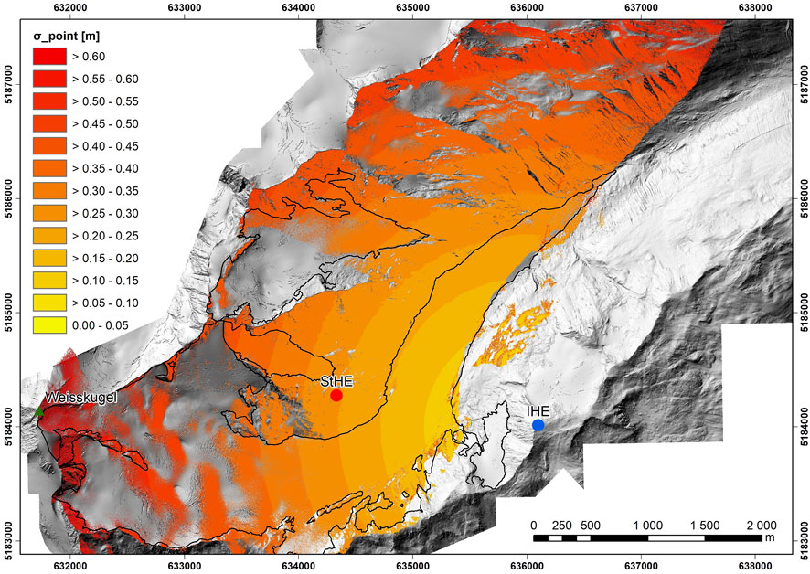
FIGURE 9. Uncertainty of a single laser pulse distributed over the glacier (σ_point).

The total uncertainty of the DEMs strongly depends on the point density. The point density found in Figure 10 is between 1 point m⁻² in the accumulation zone, furthest away from the TLS and above 13 points m⁻² directly at the glacier in the line between IHE and StHE.

FIGURE 10

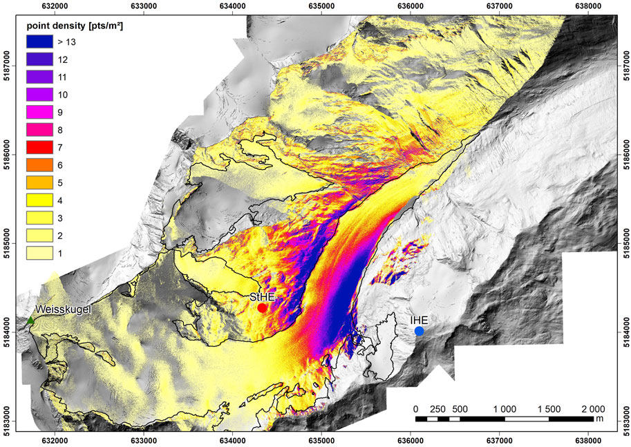
FIGURE 10. Point density in points m⁻² from IHE. The dark purple areas have point densities $>$13 points m⁻².

The total uncertainty of the DEMs improves if the point density is taken into account (Eq. 2; Figure 11). The uncertainty at the glacier tongue closest to the TLS is only 0.012 m but remains at 0.66 m in the accumulation zone. This is caused by the low point density of one or two points m⁻² in the accumulation zone, and thus, the uncertainty is close to the value found in Figure 9.

FIGURE 11

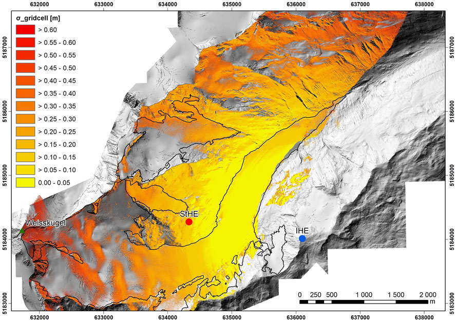
FIGURE 11. Distributed TLS uncertainty with the point density taken into account (σ_gridcell).

In the calculation of the total uncertainty of the DEMs, the registration uncertainty cannot be accounted for (Sect. 3.2). Nevertheless, the registration uncertainty with ICP_RiSCAN is in the order of a few centimeters, whereas it is in the order of decimeters for ICP_HEF. As the uncertainty of the registration method is taken as an average over the 20 areas of 100 by 100 m (Sect. 3.2), the effect of the instrument and hardware limitations is evened out and is not visible anymore. Thus, in Figure 2B, the apparent uncertainty sources are the uncertainties caused by the atmospheric conditions, the scanning geometry, rasterization, and registration. The same accounts for Figure 2A but with a smaller contribution for registration. Nevertheless, the theoretically calculated σ_cell in Figure 11 could be a few decimeters larger if the registration uncertainty from Figure 2B is taken into account, but this only applies for large anomalies in pitch measurements relative to a reference scan. Furthermore, the value of 0.008° in Eq. 5 is fairly generously chosen, and the contribution of σ_instrument to the total uncertainty budget is probably smaller. The consequences of the different uncertainties obtained on the ability to detect surface changes at the glacier are discussed in Sect. 4.

4 Detecting phenomena at the glacier surface

The aim of the installation of the TLS is to measure glacier surface changes at HEF. This section discusses a series of different phenomena that involve glacier surface changes with their appurtenant time scales, albeit having different magnitudes and can possibly be detected with a TLS.

The ability to measure the annual geodetic mass balance with a TLS has already been proven in other studies (Fischer et al., 2016; Wang et al., 2018; Xu et al., 2019). The geodetic method is comparable to the glaciological method under the assumption that we integrate over all the processes that lead to elevation changes at any single point of the glacier over the total glacier area (Kuhn et al., 1999; Zemp et al., 2010; Klug et al., 2018). The geodetic mass balances derived from the automatically registered TLS data were compared to the glaciological mass balances for the hydrological years (between 1 October and 30 September) 2016/17 to 2019/20 for HEF. Differences of −117 kg·m⁻² (mean) and 162 kg·m⁻² (root-mean-square error) were found. This is within in the glaciological mass balance uncertainty, which is quantified at ±210 kg·m⁻² for HEF (Klug et al., 2018). Thus, reanalysis (Zemp et al., 2013) or better registration is not needed and also shows the applicability of the automatically registered TLS data for yearly mass balance measurements at HEF.

The glacier mass balance can likewise be measured over seasons (Gabbud et al., 2015; Xu et al., 2019; Li et al., 2021), months, weeks, and potentially days with a TLS, given snow density information is available. This is especially interesting during the melt season, where melt evolves quickly, and snow is distributed as patches over the glacier. This can be useful validation data for atmospheric (Goger et al., 2022), snow cover (Mernild et al., 2006), or distributed mass balance models (Klok and Oerlemans, 2002; Hock and Holmgren, 2005; Machguth et al., 2006) and has magnitudes between centimeters and meters. Additionally, with daily measurements, the glacier loss day can be determined, which is the day in the hydrological year when the volume and, with similar snow distribution patterns, the mass is the same as that on 1 October. This means that after this date, the glacier will only lose mass in the present climate conditions.

On shorter time scales, the process with a magnitude of centimeters to meters at the glacier is snowfall. During snowfall events, snow is not evenly distributed over the glacier but is mostly driven by orographic precipitation in winter and by two precipitation processes that are mainly terrain and wind-driven, namely, 1) snowfall enhancement caused by the interaction with the local flow field and local cloud formation processes (Mott et al., 2014) and 2) pure particle flow interaction (preferential deposition of snowfall) (Lehning et al., 2008). After snowfall, the snow is redistributed over the glacier. These snow drift phenomena have a vertical spatial scale of $<$1 m (Filhol and Sturm, 2015) and a horizontal spatial scale of 1–100 m (Marsh et al., 2020). Depending on the atmospheric conditions, snow drifts and settles after snowfall (Mott et al., 2018). During the day, snow fall and redistribution are still hard to model, but the TLS data can be a useful tool to validate models that take them into account. Snow fall, redistribution, and snow settling are difficult to distinguish from each other as they happen simultaneously, so these are partly combined in the investigation of snow distribution.

Last, special cases of snow redistribution are avalanches. Avalanches can occur within seconds but have magnitudes up to meters in the vertical direction and runout lengths of meters to kilometers. The avalanches are clearly visible in webcam pictures at HEF, yet the DEMs give quantitative information, which is of interest for the snow avalanche community as the input for model calibration (Prokop et al., 2008; Schaffhauser et al., 2008; Hancock et al., 2020).

Our study shows the possibility to investigate the mentioned phenomena. First, on longer time scales, processes with magnitudes in the order of meters can be detected with the automatically registered data.

Second, this automated registration is also helpful to select case studies and to qualify days when glacier surface changes have occurred. Subsequently, the scans taken at these days can be post-processed with RiSCAN PRO, delivering an uncertainty of the TLS data of ±0.10 m. Moreover, the grid size in this study is set to 1 m, but to achieve the best combination between accuracy and spatial horizontal resolution, the grid size can also be set an order of magnitude larger. A coarser horizontal resolution increases the amount of measurements per grid cell and hence leads to a smaller contribution of the instrument and hardware limitations to the uncertainty budget as these are evened out in the data. Eventually, this leads to a more accurate automatically registered DEM, which is still usable in the generally coarser models, though having a lower horizontal spatial resolution.

Nevertheless, it is known that snow drift mainly occurs at mountain crests to leeward slopes (Mott et al., 2018), and these areas have an insufficient coverage and a rather low point density (1–2 points m⁻²) in the data of HEF. Therefore, future research could benefit from the coverage of the glacier accumulation zone with airborne laser scanning (ALS), which has already been done in the past at HEF at annual and seasonal temporal resolution (Helfricht et al., 2014; Klug et al., 2018). These studies can be improved with more frequent acquisitions, which might be feasible with uncrewed aerial vehicles (UAVs) (Zieher et al., 2019).

5 Comparison to other studies

The uncertainty sources discussed in this study were separately assessed in previous studies and in different contexts. The scanning geometry has been evaluated for a TLS on short ranges (≤50 m) inside a building (Soudarissanane et al., 2011). The focus in this study was on point cloud quality, when incidence angles are unfavorable and scanning ranges are long. Similar to our study, Soudarissanane et al. (2011) found that larger incidence angles lead to larger noise levels and a higher uncertainty in the position of the laser beam. Likewise, the extent of the footprint for an ALS acquisition was investigated (Schaer et al., 2007). The estimation of the uncertainty of the footprint in our study is based on the study by Schaer et al. (2007) (Eq. 18), even though the scanning geometry in an ALS acquisition is more favorable due its more perpendicular and closer range ($<$1,000 m) to the surface than the permanent TLS setup. On the other hand, TLS has no positioning errors related to the GPS/INS navigation of the airborne carrier.

The instrument and hardware limitations of TLS systems are also assessed in other studies (Lichti and Licht, 2006; Griebel et al., 2015), but they use different systems. The radial stripes found in our study have only been mentioned by Kuschnerus et al. (2021), but the cause of the stripes was not investigated.

The uncertainty caused by the atmosphere has previously been modeled in an idealized situation by Friedli (2020). This study investigated the velocity difference and refraction of the laser beam due to atmospheric conditions. The differences in the laser beam found by Friedli (2020) range between −0.11 and 0.27 m at a longest simulated distance of 1,841 m and, thus, an order of magnitude smaller than that found in our study. Friedli (2020) also stated that the change strongly depends on the temperature profile in the boundary layer. We assumed a linear temperature profile in the last 10 m of the laser beam path based on the simulated temperature at 2 m and the surface temperature. Different temperature profiles for these last meters of the laser beam path have also been tried, but no significant influences on the laser beam properties were found. Furthermore, our setting is not an idealized situation, and the temperature changes at one point in time are smaller than that in an idealized situation. In our study, the refraction of the laser beam has not been investigated, as the interpolation of the derivative of the refractive index perpendicular to the path $\frac{dn(s)}{dq}$ (Eq. 11) is not accurate in a simulation with a horizontal grid spacing of 48 m. The maximum change in the refraction angle found by Friedli (2020) is 6.3 mgon, but this strongly depends on the distance and temperature profile in the boundary layer. The refraction angle change of 6.3 mgon equals 0.0057°, which is approximately the same order of magnitude as the uncertainty added by the instrument and hardware limitations. Under the assumption that the boundary layer temperature profile is weak on a snow-covered glacier, the contribution of the angle of refraction is likely less strong than that found by Friedli (2020) and makes the laser beam hit the surface within the calculated footprint. This also validates neglecting the influence of refraction of the laser beam in our study.

Eventually, our study is able to enhance the results of Friedli (2020), as the data of the atmospheric variables are based on a high-resolution simulation and variable over time. Therewith, we show the novelty of our study, where the uncertainties as assessed by different studies are combined and applied to an actual permanent long-range TLS system.

6 Conclusion

The potential of the permanent long-range TLS system at HEF for detecting glaciologically relevant surface elevation changes has been assessed. Five uncertainty sources are analyzed: the registration method, the influence of the instrument and hardware limitations of the TLS, the effect of atmospheric conditions on the laser beam, the scanning geometry, and the uncertainty caused by rasterization. The uncertainty sources are investigated separately, showing a strong dependence on the distance from the TLS to the surface. The registration method is tested with an automated ICP approach (ICP_HEF) and with commonly used RiSCAN PRO software (ICP_RiSCAN). This results in an average vertical accuracy of the TLS data of ±0.50 m with ICP_HEF and ±0.10 m with ICP_RiSCAN at grids of 100 by 100 m. The precision of the inclination sensors of the scanner cause an uncertainty between 0.09 and 0.64 m. The influence of the atmosphere on the velocity of the laser beam strongly depends on air temperature and to a lesser extent on RH and air pressure, but only has an order of magnitude of millimeters. The contribution of the scanning geometry to the uncertainty budget is approximated between 0.02 and 0.25 m. The instrument and hardware limitations cause the largest uncertainty to the TLS data. The total uncertainty with the point density of the TLS taken into account is between 0.01 m at the area between the TLS and StHE and 0.66 m in the areas close to Weißkugel.

For the annual and seasonal mass balance, the automated approach has proven to be sufficient, as the decimeter-range uncertainty is comparable to the uncertainty of the glaciological mass balance method. Phenomena smaller than a few decimeters, such as snowfall and snow distribution, can be studied after increasing the registration accuracy with post-processing. The uncertainty of the TLS system is an order of magnitude smaller than the processes of interest. Thus, snow drift phenomena with a vertical spatial scale $>$0.10 m and a horizontal spatial scale of 1–100 m can still be investigated with the data at hand. This also shows the suitability of the system setup to validate high-resolution atmospheric models that compute snow (re)distribution by wind.

Data availability statement

The raw data supporting the conclusion of this article will be made available by the authors, without undue reservation.

Author contributions

AV developed the theory and performed the computations, except the LES simulation, which has been conducted by BG. CK designed the automated registration and fine-tuned the maps. RP maintained the TLS setup together with AV. BG, MR, and GK supervised the project. AV took the lead in writing the manuscript. All authors provided critical feedback and helped shape the research, analysis, and manuscript.

Funding

This research is embedded in the SCHISM project (Snow Cover dynamics and High-resolution Modeling) and is funded by the Austrian Science Fund (FWF) and the German Research Foundation (DFG) research project I3841-N32 Snow Cover Dynamics and Mass Balance on Mountain Glaciers. Further funding is acquired from the Universität Innsbruck.

Acknowledgments

The authors would like to thank Rudolf Sailer (Universität Innsbruck) for the help with the use of RiSCAN PRO and Katharina Anders (University of Heidelberg) for the script that enables the reading of the inclination data.

Conflict of interest

The authors declare that the research was conducted in the absence of any commercial or financial relationships that could be construed as a potential conflict of interest.

Publisher’s note

All claims expressed in this article are solely those of the authors and do not necessarily represent those of their affiliated organizations, or those of the publisher, the editors, and the reviewers. Any product that may be evaluated in this article, or claim that may be made by its manufacturer, is not guaranteed or endorsed by the publisher.

Footnotes

¹https://www.foto-webcam.eu/webcam/hintereisferner1/

References

Anders, K., Lindenbergh, R. C., Vos, S. E., Mara, H., de Vries, S., and Höfle, B. (2019). High-frequency 3D geomorphic observation using hourly terrestrial laser scanning data of a sandy beach. ISPRS Ann. Photogrammetry, Remote Sens. Spatial Inf. Sci. IV-2/W5, 317–324. doi:10.5194/isprs-annals-iv-2-w5-317-2019

CrossRef Full Text | Google Scholar

Ayala, A., Pellicciotti, F., and Shea, J. M. (2015). Modeling 2 m air temperatures over mountain glaciers: Exploring the influence of katabatic cooling and external warming. J. Geophys. Res. Atmos. 120, 3139–3157. doi:10.1002/2015jd023137

CrossRef Full Text | Google Scholar

Besl, P., and McKay, N. D. (1992). A method for registration of 3-d shapes. IEEE Trans. Pattern Analysis Mach. Intell. 14, 239–256. doi:10.1109/34.121791

CrossRef Full Text | Google Scholar

Blümcke, A., and Hess, H. (1899). Untersuchungen am Hintereisferner. Zeitschrift des deutschen und österreichischen Alpenvereins.

Google Scholar

Campos, M. B., Litkey, P., Wang, Y., Chen, Y., Hyyti, H., Hyyppä, J., et al. (2021). A long-term terrestrial laser scanning measurement station to continuously monitor structural and phenological dynamics of boreal forest canopy. Front. Plant Sci. 11, 606752. doi:10.3389/fpls.2020.606752

PubMed Abstract | CrossRef Full Text | Google Scholar

Carturan, L., Cazorzi, F., and Fontana, G. D. (2012). Distributed mass-balance modelling on two neighbouring glaciers in Ortles-Cevedale, Italy, from 2004 to 2009. J. Glaciol. 58, 467–486. doi:10.3189/2012jog11j111

CrossRef Full Text | Google Scholar

Cogley, J. G., Hock, R., Rasmussen, L., Arendt, A., Bauder, A., Braithwaite, R., et al. (2011). Glossary of glacier mass balance and related terms. IHP-VII Tech. documents hydrology 86.

Google Scholar

Conrad, O., Bechtel, B., Bock, M., Dietrich, H., Fischer, E., Gerlitz, L., et al. (2015). System for automated geoscientific analyses (SAGA) v. 2.1.4. Geosci. Model Dev. 8, 1991–2007. doi:10.5194/gmd-8-1991-2015

CrossRef Full Text | Google Scholar

Cuffey, K. M., and Paterson, W. S. B. (2010). The physics of glaciers. Oxford): Elsevier.

Google Scholar

Deruyter, G., De Sloover, L., Verbeurgt, J., De Wulf, A., and Vos, S. (2020). Macrotidal beach monitoring (Belgium) using hypertemporal terrestrial lidar. FIG Work. Week 2020 Smart Surv. land water Manag. Proc. 13.

Google Scholar

Dong, Z., Liang, F., Yang, B., Xu, Y., Zang, Y., Li, J., et al. (2020). Registration of large-scale terrestrial laser scanner point clouds: A review and benchmark. ISPRS J. Photogrammetry Remote Sens. 163, 327–342. doi:10.1016/j.isprsjprs.2020.03.013

CrossRef Full Text | Google Scholar

Fey, C., and Wichmann, V. (2016). Long-range terrestrial laser scanning for geomorphological change detection in alpine terrain - handling uncertainties. Earth Surf. Process. Landforms 42, 789–802. doi:10.1002/esp.4022

CrossRef Full Text | Google Scholar

Filhol, S., and Sturm, M. (2015). Snow bedforms: A review, new data, and a formation model. J. Geophys. Res. Earth Surf. 120, 1645–1669. doi:10.1002/2015jf003529

CrossRef Full Text | Google Scholar

Fischer, M., Huss, M., Kummert, M., and Hoelzle, M. (2016). Application and validation of long-range terrestrial laser scanning to monitor the mass balance of very small glaciers in the Swiss Alps. Cryosphere 10, 1279–1295. doi:10.5194/tc-10-1279-2016

CrossRef Full Text | Google Scholar

Friedli, E. (2020). Point cloud registration and mitigation of refraction effects for geomonitoring using long-range terrestrial laser scanning. Ph.D. thesis. Zurich: ETH Zurich. doi:10.3929/ETHZ-B-000409052

CrossRef Full Text | Google Scholar

Fritzmann, P., Höfle, B., Vetter, M., Sailer, R., Stötter, J., and Bollmann, E. (2011). Surface classification based on multi-temporal airborne LiDAR intensity data in high mountain environments, a case study from Hintereisferner, Austria. Z. für Geomorphol. Suppl. Issues 55, 105–126. doi:10.1127/0372-8854/2011/0055s2-0048

CrossRef Full Text | Google Scholar

Gabbud, C., Micheletti, N., and Lane, S. N. (2015). Lidar measurement of surface melt for a temperate alpine glacier at the seasonal and hourly scales. J. Glaciol. 61, 963–974. doi:10.3189/2015jog14j226

CrossRef Full Text | Google Scholar

Gardner, A. S., Moholdt, G., Cogley, J. G., Wouters, B., Arendt, A. A., Wahr, J., et al. (2013). A reconciled estimate of glacier contributions to sea level rise: 2003 to 2009. science 340, 852–857. doi:10.1126/science.1234532

PubMed Abstract | CrossRef Full Text | Google Scholar

Geist, T., and Stötter, J. (2007). Documentation of glacier surface elevation change with multi-temporal airborne laser scanner data–case study: Hintereisferner and Kesselwandferner, Tyrol, Austria. Z. fur Gletscherkd. Glazialgeol. 41, 77–106.

Google Scholar

Goger, B., Stiperski, I., Nicholson, L., and Sauter, T. (2022). Large-eddy simulations of the atmospheric boundary layer over an Alpine glacier: Impact of synoptic flow direction and governing processes. Q. J. R. Meteorological Soc. 148, 1319–1343. doi:10.1002/qj.4263

CrossRef Full Text | Google Scholar

Greuell, W., and Böhm, R. (1998). 2 m temperatures along melting mid-latitude glaciers, and implications for the sensitivity of the mass balance to variations in temperature. J. Glaciol. 44, 9–20. doi:10.1017/s0022143000002306

CrossRef Full Text | Google Scholar

Griebel, A., Bennett, L. T., Culvenor, D. S., Newnham, G. J., and Arndt, S. K. (2015). Reliability and limitations of a novel terrestrial laser scanner for daily monitoring of forest canopy dynamics. Remote Sens. Environ. 166, 205–213. doi:10.1016/j.rse.2015.06.014

CrossRef Full Text | Google Scholar

Gurgiser, W., Mölg, T., Nicholson, L., and Kaser, G. (2013). Mass-balance model parameter transferability on a tropical glacier. J. Glaciol. 59, 845–858. doi:10.3189/2013jog12j226

CrossRef Full Text | Google Scholar

Hancock, H., Eckerstorfer, M., Prokop, A., and Hendrikx, J. (2020). Quantifying seasonal cornice dynamics using a terrestrial laser scanner in Svalbard, Norway. Nat. Hazards Earth Syst. Sci. 20, 603–623. doi:10.5194/nhess-20-603-2020

CrossRef Full Text | Google Scholar

Helfricht, K., Kuhn, M., Keuschnig, M., and Heilig, A. (2014). Lidar snow cover studies on glaciers in the ötztal Alps (Austria): Comparison with snow depths calculated from GPR measurements. Cryosphere 8, 41–57. doi:10.5194/tc-8-41-2014

CrossRef Full Text | Google Scholar

Hock, R., and Holmgren, B. (2005). A distributed surface energy-balance model for complex topography and its application to Storglaciären, Sweden. J. Glaciol. 51, 25–36. doi:10.3189/172756505781829566

CrossRef Full Text | Google Scholar

Joerg, P. C., Morsdorf, F., and Zemp, M. (2012). Uncertainty assessment of multi-temporal airborne laser scanning data: A case study on an alpine glacier. Remote Sens. Environ. 127, 118–129. doi:10.1016/j.rse.2012.08.012

CrossRef Full Text | Google Scholar

Kaasalainen, S., Kaartinen, H., and Kukko, A. (2008). Snow cover change detection with laser scanning range and brightness measurements. EARSeL eProceedings 7.

Google Scholar

Kaser, G., Fountain, A., and Jansson, P. (2003). A manual for monitoring the mass balance of mountain glaciers. Paris: UNESCO.

Google Scholar

Klok, E. L., and Oerlemans, J. (2002). Model study of the spatial distribution of the energy and mass balance of Morteratschgletscher, Switzerland. J. Glaciol. 48, 505–518. doi:10.3189/172756502781831133

CrossRef Full Text | Google Scholar

Klug, C., Bollmann, E., Galos, S. P., Nicholson, L., Prinz, R., Rieg, L., et al. (2018). Geodetic reanalysis of annual glaciological mass balances (2001–2011) of Hintereisferner, Austria. Cryosphere 12, 833–849. doi:10.5194/tc-12-833-2018

CrossRef Full Text | Google Scholar

Kromer, R. A., Abellán, A., Hutchinson, D. J., Lato, M., Chanut, M.-A., Dubois, L., et al. (2017). Automated terrestrial laser scanning with near-real-time change detection – monitoring of the Séchilienne landslide. Earth Surf. Dyn. 5, 293–310. doi:10.5194/esurf-5-293-2017

CrossRef Full Text | Google Scholar

Kuhn, M., Dreiseitl, E., Hofinger, S., Markl, G., Span, N., and Kaser, G. (1999). Measurements and models of the mass balance of Hintereisferner. Geogr. Ann. Ser. A Phys. Geogr. 81, 659–670. doi:10.1111/j.0435-3676.1999.00094.x

CrossRef Full Text | Google Scholar

Kuschnerus, M., Schröder, D., and Lindenbergh, R. (2021). “Environmental influences on the stability of a permanently installed laser scanner,” in The international archives of the photogrammetry, remote sensing and spatial information Sciences, XLIII-B2-2021, 745–752. doi:10.5194/isprs-archives-xliii-b2-2021-745-2021

CrossRef Full Text | Google Scholar

Laserdata (2022). LIS pro 3D software package.

Google Scholar

Lehning, M., Löwe, H., Ryser, M., and Raderschall, N. (2008). Inhomogeneous precipitation distribution and snow transport in steep terrain. Water Resour. Res. 44. doi:10.1029/2007wr006545

CrossRef Full Text | Google Scholar

Li, H., Wang, P., Li, Z., Jin, S., Xu, C., Liu, S., et al. (2021). An application of three different field methods to monitor changes in Urumqi Glacier No. 1, Chinese Tien Shan, during 2012–18. J. Glaciol. 68, 41–53. doi:10.1017/jog.2021.71

CrossRef Full Text | Google Scholar

Lichti, D. D., and Licht, M. G. (2006). Experiences with terrestrial laser scanner modelling and accuracy assessment. Int. Archives Photogrammetry, Remote Sens. Spatial Inf. Sci. 36, 155–160.

Google Scholar

Lichti, J., D., and Skaloud, (2010). “Registration and calibration,” in Airborne and terrestrial laser scanning. Editors H. Vosselman, George, and Maas (Dunbeath: Whittles Publishing), 83–133.

Google Scholar

Machguth, H., Paul, F., Hoelzle, M., and Haeberli, W. (2006). Distributed glacier mass-balance modelling as an important component of modern multi-level glacier monitoring. Ann. Glaciol. 43, 335–343. doi:10.3189/172756406781812285

CrossRef Full Text | Google Scholar

Marsh, C. B., Pomeroy, J. W., Spiteri, R. J., and Wheater, H. S. (2020). A finite volume blowing snow model for use with variable resolution meshes. Water Resour. Res. 56. doi:10.1029/2019wr025307

CrossRef Full Text | Google Scholar

Mernild, S. H., Liston, G. E., Hasholt, B., and Knudsen, N. T. (2006). Snow distribution and melt modeling for mittivakkat glacier, ammassalik island, southeast Greenland. J. Hydrometeorol. 7, 808–824. doi:10.1175/jhm522.1

CrossRef Full Text | Google Scholar

Mölg, T., Maussion, F., Yang, W., and Scherer, D. (2012). The footprint of Asian monsoon dynamics in the mass and energy balance of a Tibetan glacier. Cryosphere 6, 1445–1461. doi:10.5194/tc-6-1445-2012

CrossRef Full Text | Google Scholar

Mott, R., Scipión, D., Schneebeli, M., Dawes, N., Berne, A., and Lehning, M. (2014). Orographic effects on snow deposition patterns in mountainous terrain. J. Geophys. Res. Atmos. 119, 1419–1439. doi:10.1002/2013jd019880

CrossRef Full Text | Google Scholar

Mott, R., Stiperski, I., and Nicholson, L. (2020). Spatio-temporal flow variations driving heat exchange processes at a mountain glacier. Cryosphere 14, 4699–4718. doi:10.5194/tc-14-4699-2020

CrossRef Full Text | Google Scholar

Mott, R., Vionnet, V., and Grünewald, T. (2018). The seasonal snow cover dynamics: Review on wind-driven coupling processes. Front. Earth Sci. 6. doi:10.3389/feart.2018.00197

CrossRef Full Text | Google Scholar

Pfeifer, N., Mandlburger, G., Otepka, J., and Karel, W. (2014). Opals – A framework for airborne laser scanning data analysis. Comput. Environ. Urban Syst. 45, 125–136. doi:10.1016/j.compenvurbsys.2013.11.002

CrossRef Full Text | Google Scholar

Prinz, R., Nicholson, L. I., Mölg, T., Gurgiser, W., and Kaser, G. (2016). Climatic controls and climate proxy potential of Lewis Glacier, Mt. Kenya. Cryosphere 10, 133–148. doi:10.5194/tc-10-133-2016

CrossRef Full Text | Google Scholar

Prokop, A., and Panholzer, H. (2009). Assessing the capability of terrestrial laser scanning for monitoring slow moving landslides. Nat. Hazards Earth Syst. Sci. 9, 1921–1928. doi:10.5194/nhess-9-1921-2009

CrossRef Full Text | Google Scholar

Prokop, A., Schirmer, M., Rub, M., Lehning, M., and Stocker, M. (2008). A comparison of measurement methods: Terrestrial laser scanning, tachymetry and snow probing for the determination of the spatial snow-depth distribution on slopes. Ann. Glaciol. 49, 210–216. doi:10.3189/172756408787814726

CrossRef Full Text | Google Scholar

RIEGL (2019a). Datasheet RIEGL VZ-6000. RIEGL laser measurement systems. Horn, Austria.

Google Scholar

RIEGL (2019b). RiSCAN PRO. RIEGL laser measurement systems. 2.8.0 edn. Horn, Austria.

Google Scholar

RIEGL (2013). RiVLib. RIEGL laser measurement systems. 1.13 edn. Horn, Austria.

Google Scholar

Schaer, P., Skaloud, J., Landtwing, S., and Legat, K. (2007). “Accuracy estimation for laser point cloud including scanning geometry,” in Mobile Mapping Symposium 2007, Padova, Italy (Padova).

Google Scholar

Schaffhauser, A., Adams, M., Fromm, R., Jörg, P., Luzi, G., Noferini, L., et al. (2008). Remote sensing based retrieval of snow cover properties. Cold Regions Sci. Technol. 54, 164–175. doi:10.1016/j.coldregions.2008.07.007

CrossRef Full Text | Google Scholar

Sheng, Y. (2008). Quantifying the size of a lidar footprint: A set of generalized equations. IEEE Geoscience Remote Sens. Lett. 5, 419–422. doi:10.1109/lgrs.2008.916978

CrossRef Full Text | Google Scholar

Soudarissanane, S., Lindenbergh, R., Menenti, M., and Teunissen, P. (2011). Scanning geometry: Influencing factor on the quality of terrestrial laser scanning points. ISPRS J. Photogrammetry Remote Sens. 66, 389–399. doi:10.1016/j.isprsjprs.2011.01.005

CrossRef Full Text | Google Scholar

Soudarissanane, S. (2016). The geometry of terrestrial laser scanning; identification of errors, modeling and mitigation of scanning geometry. Delft: Delft University of Technology. Ph.D. thesis. doi:10.4233/UUIDB7AE0BD3-23B8-4A8A-9B7D-5E494EBB54E5

CrossRef Full Text | Google Scholar

Span, N., Kuhn, M. H., and Schneider, H. (1997). 100 years of ice dynamics of hintereisferner, central Alps, Austria, 1894–1994. Ann. Glaciol. 24, 297–302. doi:10.3189/s0260305500012349

CrossRef Full Text | Google Scholar

Strasser, U., Marke, T., Braun, L., Escher-Vetter, H., Juen, I., Kuhn, M., et al. (2018). The rofental: A high alpine research basin (1890—3770 m a.s.l.) in the ötztal Alps (Austria) with over 150 years of hydrometeorological and glaciological observations. Earth Syst. Sci. Data 10, 151–171. doi:10.5194/essd-10-151-2018

CrossRef Full Text | Google Scholar

Voordendag, A. B., Goger, B., Klug, C., Prinz, R., Rutzinger, M., and Kaser, G. (2021). “Automated and permanent long-range terrestrial laser scanning in a high mountain environment: Setup and first results,” in ISPRS annals of the photogrammetry, remote sensing and spatial information Sciences, V-2-2021, 153–160. doi:10.5194/isprs-annals-v-2-2021-153-2021

CrossRef Full Text | Google Scholar

Vos, S., Lindenbergh, R., and de Vries, S. (2017). Coastscan: Continuous monitoring of coastal change using terrestrial laser scanning. Coast. Dyn. 233, 1518–1528.

Google Scholar

Wang, F., Xu, C., Li, Z., Anjum, M. N., and Wang, L. (2018). Applicability of an ultra-long-range terrestrial laser scanner to monitor the mass balance of Muz Taw Glacier, Sawir Mountains, China. Sci. Cold Arid Regions 10, 47–54. doi:10.3724/SP.J.1226.2018.00047

CrossRef Full Text | Google Scholar

Wehr, A., and Lohr, U. (1999). Airborne laser scanning—An introduction and overview. ISPRS J. photogrammetry remote Sens. 54, 68–82. doi:10.1016/s0924-2716(99)00011-8

CrossRef Full Text | Google Scholar

Xu, C., Li, Z., Li, H., Wang, F., and Zhou, P. (2019). Long-range terrestrial laser scanning measurements of annual and intra-annual mass balances for Urumqi Glacier No. 1, eastern Tien Shan, China. Cryosphere 13, 2361–2383. doi:10.5194/tc-13-2361-2019

CrossRef Full Text | Google Scholar

Zemp, M., Hoelzle, M., and Haeberli, W. (2009). Six decades of glacier mass-balance observations: A review of the worldwide monitoring network. Ann. Glaciol. 50, 101–111. doi:10.3189/172756409787769591

CrossRef Full Text | Google Scholar

Zemp, M., Jansson, P., Holmlund, P., Gärtner-Roer, I., Koblet, T., Thee, P., et al. (2010). Reanalysis of multi-temporal aerial images of Storglaciären, Sweden (1959–99) – part 2: Comparison of glaciological and volumetric mass balances. Cryosphere 4, 345–357. doi:10.5194/tc-4-345-2010

CrossRef Full Text | Google Scholar

Zemp, M., Thibert, E., Huss, M., Stumm, D., Denby, C. R., Nuth, C., et al. (2013). Reanalysing glacier mass balance measurement series. Cryosphere 7, 1227–1245. doi:10.5194/tc-7-1227-2013

CrossRef Full Text | Google Scholar

Zevenbergen, L. W., and Thorne, C. R. (1987). Quantitative analysis of land surface topography. Earth Surf. Process. Landforms 12, 47–56. doi:10.1002/esp.3290120107

CrossRef Full Text | Google Scholar

Zieher, T., Bremer, M., Rutzinger, M., Pfeiffer, J., Fritzmann, P., and Wichmann, V. (2019). Assessment of landslide-induced displacement and deformation of above-ground objects using uav-borne and airborne laser scanning data. ISPRS Ann. Photogrammetry, Remote Sens. Spatial Inf. Sci. IV-2/W5, 461–467. doi:10.5194/isprs-annals-iv-2-w5-461-2019

CrossRef Full Text | Google Scholar