Synthesizing magnetotelluric time series based on forward modeling

Introduction

The magnetotelluric (MT) method is widely used in the surface geological survey, mineral resources exploration, earthquake, volcano, and continental dynamics by detecting subsurface electrical structures (Cai et al., 2017; Jiang et al., 2022). The time series of the electric and magnetic fields are collected simultaneously at the surface and the MT response is subsequently obtained by Fourier transform and transfer function estimation. High quality transfer function estimation is a prerequisite for reliable detection of subsurface structures. With the development of industrialization, MT hardware devices have been perfected to collect reliable raw data. However, industrialization also makes artificial noise increase, which seriously affects the quality of measurement data and limits the application of MT method (Szarka, 1988; Junge, 1996; Banks, 1998). Existing time series processing techniques, such as the least-square method (Sims et al., 1971), remote reference method (Goubau et al., 1978; Gamble et al., 1979b; Gamble et al., 1979a), robust estimation method (Egbert and Booker, 1986; Chave et al., 1987; Larsen et al., 1996; Smirnov, 2003; Chave and Thomson, 2004), maximum likelihood estimation method (Chave, 2014; Chave, 2017), and others methods based on wavelet transform, Hilbert-Huang transform, variational mode decomposition, and inter-station transfer function (Kappler, 2012; Cai, 2014; Campanya et al., 2014; Cai and Chen, 2015; Carbonari et al., 2017; Wang et al., 2017), have different processing performance for different kinds of noise. For example, the least-square method performs poorly in the presence of outliers (Egbert and Booker, 1986), and the remote reference method does not work when noise is correlated at the local and remote sites (Shalivahan and Bhattacharya, 2002; Pomposiello et al., 2009), and the robust estimation method usually fails to work when MT data are contaminated by persistent or coherent noises (Escalas et al., 2013; Carbonari et al., 2017; Li et al., 2020a; Li et al., 2020c; Zhou et al., 2022; Zhang et al., 2022). New time series processing methods for various types of noise are the focus of current research, but there is a lack of criteria to evaluate the effectiveness of various MT time series processing methods in existing studies. The traditional evaluation method based on curve continuity is proved to be unreliable (Sutarno, 2005). Many studies take the measured low-noise data as the standard data, but because the real response is unknown, it is insufficient to prove the effectiveness of the time series processing method (Li et al., 2020a; Li et al., 2020b; Guo et al., 2022; Zhou et al., 2022). Therefore, reliable standard time series are urgently needed to test the effectiveness of various time series processing methods.

In geophysical inversion, the validity of the inversion method is assessed by comparing the inversion results with a given evaluation model. Similarly, if the time series of the evaluated model are available, they can be used to test the performance of different time series processing methods. Several studies have proposed techniques for synthesizing time series of simple models. For example, Varentsov and Sokolova (1995) and Loddo et al. (2002) realized the synthetic time series techniques based on inverse Fourier transform and convolution. These techniques take the measured low-noise magnetic field data or random number sequences as the synthetic magnetic field time series, and then use the impedance of a one-dimensional (1D) or two-dimensional (2D) model to calculate the electric field time series. However, the given time series may be noisy and its true model is unknown or even non-existent, so their synthetic time series are unreliable. Moreover, these techniques are also difficult to simulate the variability of the actual natural sources of the electromagnetic field. Kelbert et al. (2017) predicted the geoelectric field from the impedance of the 3D model and the time series of the magnetic storm, which was highly consistent with the measured data. This is a nice advance for synthesizing time series of complex models, but the method also relies on a given time series.

In this paper, we propose a method to synthesize MT time series based on forward modeling. All five-channel time series are generated by forward modeling, which accurately reflects the spatial distribution and temporal variability properties of the electromagnetic fields in the model. The transfer function can be obtained by processing synthetic time series using common software, so that the actual observed time series can be adequately simulated. In the following paper, the basic principles and implementation of the method are detailed. The time series of the 1D and 3D models are then synthesized in this way. Commercial and open-source software is used to process and analyze the synthetic time series. The processing results of the time series and the response of a given model are compared to verify the reliability of the synthetic time series. Finally, noise is added to the synthetic time series to test the performance of different data processing methods, demonstrating that the synthetic time series can be used as an evaluation criterion for data processing techniques.

Methodology

Theory of synthesizing time series

The time domain form of the single-frequency electromagnetic field is (detailed derivation is in the Supplementary Material S1):

$\left\{,\begin{array}{c}\mathbf{e}\left(\omega ,t\right)={\mathbf{A}}_e\cos \left(\omega t+{\mathrm{\Phi }}_e\right)\hfill \\ \mathbf{h}\left(\omega ,t\right)={\mathbf{A}}_h\cos \left(\omega t+{\mathrm{\Phi }}_h\right)\hfill \end{array},\right.(1)$

where ω denotes the angular frequency. A_e = |E(ω)|, A_h = |H(ω)|,Φ_e = Arg(E(ω)),Φ_h = Arg(H(ω)). E(ω) and H(ω) are the electromagnetic fields in the frequency domain, which can be calculated by MT forward modeling. Thus, Eq. 1 provides a new approach to synthesize MT time series. By MT forward modeling, E(ω) and H(ω) is calculated, which is substituted into Eq. 1 to calculate the time series of single frequency. Time series containing N frequencies can be synthesized according to the superposition principle of electromagnetic fields:

$\left\{,\begin{array}{c}\mathbf{e}\left(t\right)={\sum }_{k=1}^N\mathbf{e}\left(\omega ,t\right)\hfill \\ \mathbf{h}\left(t\right)={\sum }_{k=1}^N\mathbf{h}\left(\omega ,t\right)\hfill \end{array}\right..(2)$

Following the above theory, we can design any complex model and synthesize time series by forward modeling. The synthesized time series can be used to test the effectiveness of data processing methods.

MT forward modeling

In the approach of this paper, MT forward modeling is a prerequisite for synthesizing time series. MT forward modeling has become highly mature after several decades. Numerical simulation methods such as finite difference, finite element, integral equation, and even deep learning can solve the forward calculation of various complex models (Wang et al., 2021). Kelbert et al. (2014) developed ModEM, an open-source 3D magnetotelluric and controlled-source electromagnetic forward and inversion system, which was used for forward modeling of the 3D model in this method. We have made minor modifications to ModEM by adding an output interface for the electromagnetic field.

The transfer functions include the impedance and tipper, which are defined as follows:

$\left\{,\begin{array}{c}{E}_x\left(\omega \right)=Z_{xx}\left(\omega \right)H_x\left(\omega \right)+Z_{xy}\left(\omega \right)H_y\left(\omega \right)\hfill \\ E_y\left(\omega \right)=Z_{yx}\left(\omega \right)H_x\left(\omega \right)+Z_{yy}\left(\omega \right)H_y\left(\omega \right)\hfill \\ H_z\left(\omega \right)=T_{zx}\left(\omega \right)H_x\left(\omega \right)+T_{zy}\left(\omega \right)H_y\left(\omega \right)\hfill \end{array}\right..(3)$

Eq. 3 can be abbreviated as E = ZH and H_z = TH, where Z is the MT impedance tensor and T is the tipper vector. E and H is horizontal electric and magnetic field component. H_z is vertical magnetic field. The above three equations are independent and solving them requires at least two linearly independent sets of electromagnetic fields. In the forward modeling of MT, we solve the governing equations with two different polarization sources as boundary conditions and obtain two sets of fields:

Polarization 1: $E_x^1(\omega )$, $E_y^1(\omega )$, $H_x^1(\omega )$, $H_y^1(\omega )$, $H_z^1(\omega )$,

Polarization 2: $E_x^2(\omega )$, $E_y^2(\omega )$, $H_x^2(\omega )$, $H_y^2(\omega )$, $H_z^2(\omega )$.

Then combined into transfer functions:

$\left\{,\begin{array}{c}{Z}_{xy}\left(\omega \right)=\frac{E_x^2\left(\omega \right)H_x^1\left(\omega \right)-E_x^1\left(\omega \right)H_x^2\left(\omega \right)}{H_x^1\left(\omega \right)H_y^2\left(\omega \right)-H_x^2\left(\omega \right)H_y^1\left(\omega \right)}\hfill \\ Z_{xx}\left(\omega \right)=\frac{E_x^1\left(\omega \right)H_y^2\left(\omega \right)-E_x^2\left(\omega \right)H_y^1\left(\omega \right)}{H_x^1\left(\omega \right)H_y^2\left(\omega \right)-H_x^2\left(\omega \right)H_y^1\left(\omega \right)}\hfill \\ Z_{yx}\left(\omega \right)=\frac{E_y^1\left(\omega \right)H_y^2\left(\omega \right)-E_y^2\left(\omega \right)H_y^1\left(\omega \right)}{H_x^1\left(\omega \right)H_y^2\left(\omega \right)-H_x^2\left(\omega \right)H_y^1\left(\omega \right)}\hfill \\ Z_{yy}\left(\omega \right)=\frac{E_y^2\left(\omega \right)H_x^1\left(\omega \right)-E_y^1\left(\omega \right)H_x^2\left(\omega \right)}{H_x^1\left(\omega \right)H_y^2\left(\omega \right)-H_x^2\left(\omega \right)H_y^1\left(\omega \right)}\hfill \\ T_{zx}\left(\omega \right)=\frac{H_z^1\left(\omega \right)H_y^2\left(\omega \right)-H_z^2\left(\omega \right)H_y^1\left(\omega \right)}{H_x^1\left(\omega \right)H_y^2\left(\omega \right)-H_x^2\left(\omega \right)H_y^1\left(\omega \right)}\hfill \\ T_{zy}\left(\omega \right)=\frac{H_z^2\left(\omega \right)H_x^1\left(\omega \right)-H_z^1\left(\omega \right)H_x^2\left(\omega \right)}{H_x^1\left(\omega \right)H_y^2\left(\omega \right)-H_x^2\left(\omega \right)H_y^1\left(\omega \right)}\hfill \end{array}\right..(4)$

In practical MT, the time series of electromagnetic fields are collected, and divided into segments (L). For a given frequency, L groups of electromagnetic fields are obtained by Fourier transform of the time series segments. And the transfer functions can be estimated from this L groups of electromagnetic fields by estimation methods, such as the least-square method. The purpose of MT data processing is to obtain transfer functions for multiple discrete frequencies. Therefore, only time series containing the given frequencies need to be synthesized for the study of data processing methods. MT transfer function estimation requires that these sets of electromagnetic fields to be linearly independent, which is easily satisfied by the fact that the polarization direction of the natural electromagnetic field source varies with time. And this time-varying polarization needs be simulated in synthetic time series by segmentation and concatenation.

Source simulation

In the forward modeling, only the fields of two different polarization sources are calculated. The natural sources are time-varying, and the sources at different moments can be simulated by combining the two sources described above.

Any source (denoted as S) can be derived by a linear combination of two orthogonal sources (denoted as S¹ and S²): S = C¹S¹ + C²S². The fields of source S, S¹ and S² are A = (E_x, E_y, H_x, H_y, H_z), ${\mathbf{A}}^1=(E_x^1,E_y^1,H_x^1,H_y^1,H_z^1)$ and ${\mathbf{A}}^2=(E_x^2,E_y^2,H_x^2,H_y^2,H_z^2)$, respectively. The linear combination consistent with the source also holds in the fields: A = C¹A¹ + C²A². For the 1D model, the two field components (E^1D and H^1D) can be calculated by forward modeling. The fields of the two orthogonal sources are:

$\left\{\begin{array}{c}{\mathbf{A}}^1=\left(E^{1D},0,0,H^{1D},0\right)\hfill \\ {\mathbf{A}}^2=\left(0,E^{1D},-H^{1D},0,0\right)\hfill \end{array}\right..(5)$

For the 2D model, $E_x^{TE}$, $H_y^{TE}$ and $H_z^{TE}$ can be calculated by the forward modeling of the TE polarization, $E_y^{TM}$ and $H_x^{TM}$ can be calculated by the forward modeling of the TM polarization, and the two polarization sources are orthogonal. The fields are:

$\left\{\begin{array}{c}{\mathbf{A}}^1=\left(E_x^{TE},0,0,H_y^{TE},H_z^{TE}\right)\hfill \\ {\mathbf{A}}^2=\left(0,E_y^{TM},H_x^{TM},0,0\right)\hfill \end{array}\right..(6)$

For the 3D model, the full field components can be calculated by forward modeling with two orthogonal polarization sources.

After obtaining the forward modeling fields, we can use them to synthesize the time series. The synthesis procedure is described below by taking an example of a particular site, a particular frequency, and a particular time series slice of polarization 1.

First, the intensities of natural field sources in different frequency ranges is simulated. Loddo et al. (2002) used a smoothed natural source horizontal magnetic field curve to simulate the intensity. In the proposed method, the forward fields of each frequency are scaled by a uniform coefficient to be near the natural field intensity (e.g. ${\mathbf{A}}_s^1=S^1{\mathbf{A}}^1$, S¹ is the scaling coefficient of polarization 1).

Second, we use pseudo-random numbers to simulate the field source intensity and polarization variations. The $r_a^1$ and $r_p^1$ are randomly generated amplitude coefficients and phase shift. The electromagnetic field of a random field source is:

${\mathbf{A}}_r^1=r_a^1{e}^{i{r}_p^1}{S}^1{\mathbf{A}}^1.(7)$

Finally, by substituting Eq. 7 into Eq. 1, the synthetic time series of polarization 1 at the given frequency at the given site in the given segment can be generated. The time series of other sites in the model can be synthesized with the same coefficient $(r_a^1{e}^{i{r}_p^1}{S}^1)$.

Splicing time series segments

We simulate the time-varying MT signal by splicing a large number of time series segments, each generated following the procedure described above. The segmentation, synthesis, and splicing of each frequency and each polarization are performed independently before the final superposition. The length of each segment is randomly generated and needs to be long enough to preserve valid spectral information to make the transfer functions stable. After many tests, we found that stable transfer functions are obtained only when the segment length exceeds four times the period. In this approach, the segment length is generated randomly and ranges from 0 to 8 times the period by default. It can also be adjusted manually. Excessly short segments are considered noise, which is allowed in this approach.

We randomly generate the amplitude and phase of each segment, and the splice of the two segments is discontinuous. This discontinuity can be ignored as noise or suppressed by windowing at the splice. We design a Hanning window of length half a period and flip the window such that the two endpoints of the window are 1 and the midpoint is 0 (Figure 1A).After adding the window, the two segments are smoothly connected. For example, the original time series (Figure 1B) is divided into four segments. The time series after windowing (Figure 1C) is continuous and smooth.

FIGURE 1

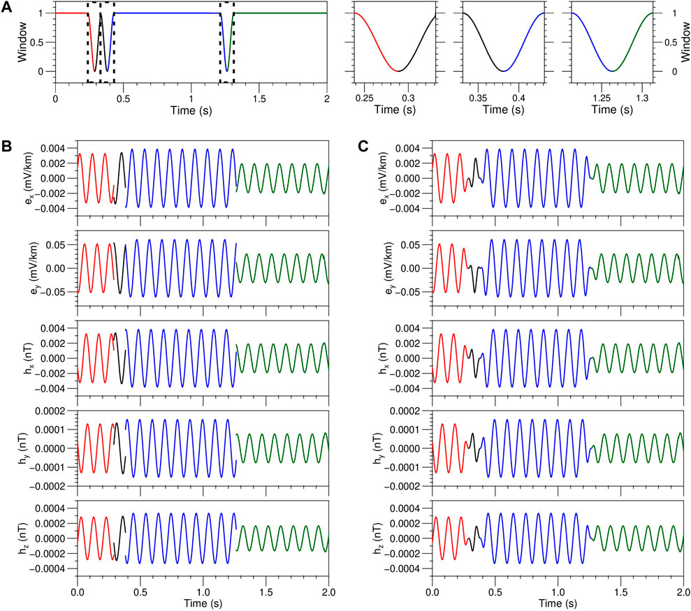
FIGURE 1. Time series splice diagram of a single frequency. The frequency is 10 Hz, the direction of source polarization is X, and the sampling rate is 2,400 Hz. (A) Window function time series, (B) original time series, and (C) windowed time series.

Figure 2 shows the synthesizing process of the time series of single frequency of H_x channel. The time series of the X-direction source is divided into four segments, whereas that of the Y-direction source is divided into two segments. The amplitude and phase of each segment are randomly generated by Eq. 7. The original time series is calculated by Eq. 1. The original time series is multiplied by the window function to obtain the windowed time series. And the windowed time series of the two sources were superimposed to get the total time series of the single frequency. The time series of multi-frequencies is the sum of all single frequencies, as shown in Figure 3.

FIGURE 2

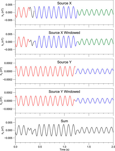
FIGURE 2. Synthesis a single frequency time series. The frequency is 10 Hz, the sampling rate is 2,400 Hz, and the field component is H_x.

FIGURE 3

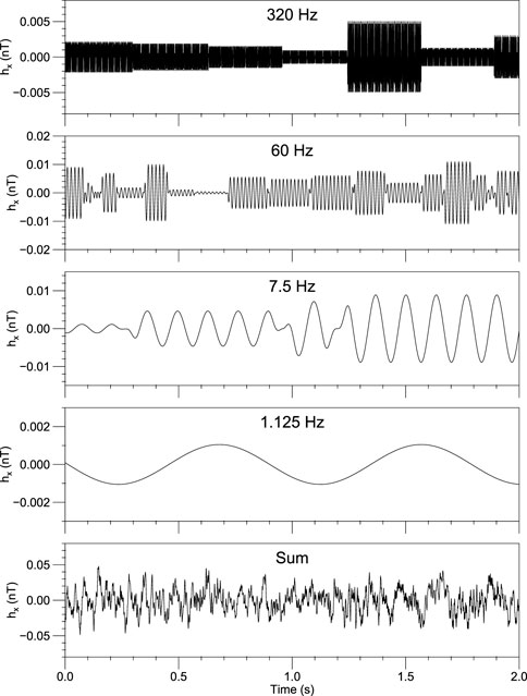
FIGURE 3. Synthesis of multi-frequency time series. The frequency ranges from 320 to 1.125 Hz, with 18 frequencies, of which only four are plotted in the figure. The sampling rate is 2,400 Hz, and the field component is H_x. The last subplot is a superimposed time series of 18 frequencies.

Synthesizing time series workflow

According to the above theory, the complete workflow of synthesizing magnetotelluric time series based on forward modeling is shown in Figure 4.

FIGURE 4

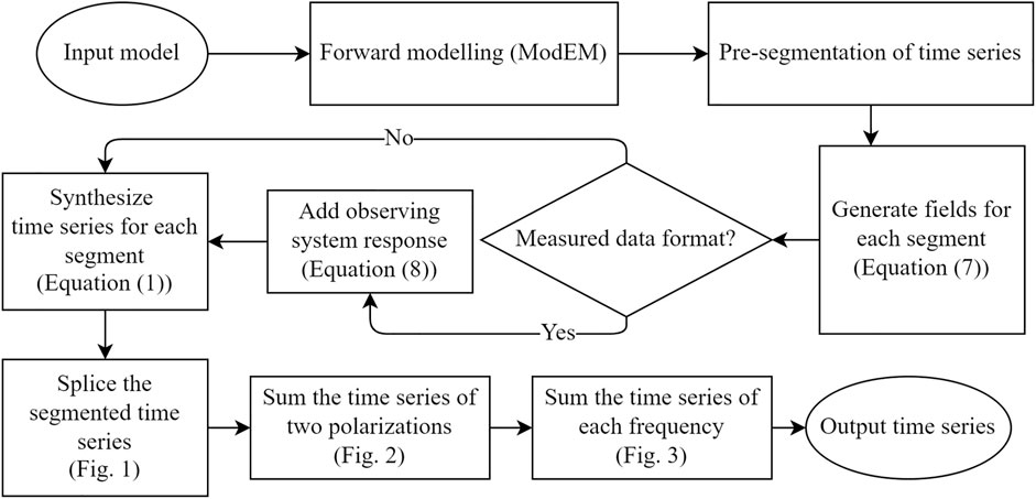
FIGURE 4. Flow chart of synthesis magnetotelluric time series based on forward modeling.

All the processes except forward modeling in Figure 4 have been implemented using Delphi language programming. The 3D forward modeling was performed using the modified ModEM code described above.

In addition, synthesizing time series in a measured data format requires the addition of the response of the observed system. In fieldwork, the measured electromagnetic field signal is recorded in a specific format according to the equipment used (e.g. Phoenix Geophysics, MTU-5A). The natural electromagnetic field signal measured by the sensor is transmitted to the instrument in the form of the electrical signals. To facilitate recording, the instrument takes an analog-to-digital conversion of this electrical signal before saving. During the conversion process, the analog-to-digital conversion coefficient (2²³ in MTU-5A) is multiplied and then rounded and stored (three-byte integer in MTU-5A). The relationship between the recorded data and the real signal is stable in the frequency domain, termed the instrument response (obtained from calibration). The instrument response is added as:

$A^o\left(\omega \right)=C{A}^r\left(\omega \right)R\left(\omega \right),(8)$

where A^r is the real signal, A^o is the output record, and R is the instrument response, C is the analog-to-digital conversion coefficient. Based on this principle, we implemented the synthesized time series with MTU-5A format as output.

Numerical experiments

1D model

To validate this approach, we first synthesized a time series of a 1D model for testing. We designed a three-layer model with resistivity of 10Ωm, 100Ωm, and 1Ωm from top to bottom, with the top two layers having thicknesses of 1 km and 10 km, respectively. We obtained the electromagnetic fields of the model through forward modeling, and the frequencies we used are approximately log-uniformly distributed, see the vertical grid in Figure 5D.

FIGURE 5

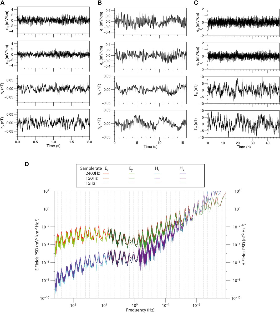
FIGURE 5. The synthetic time series and power spectrum density of the 1D model. (A) Time series with 2400Hz sampling rate, (B) Time series with 150Hz sampling rate, (C) Time series with 15Hz sampling rate, (D) power spectrum of the time series.

To avoid excessive data due to a single high sampling rate, the synthetic time series is divided into high, medium and low sampling rates of 2,400, 150, and 15 Hz using the parameters of MTU-5A. The length of the synthetic time series is 48 h, where the low sampling rate records are continuous while the high and medium sampling rate records are discontinuous. Each 300 s, a 16 s medium sampling rate record or a 2 s low sampling rate record is synthesized alternately. The synthesizing frequency ranges for high, medium, and low sampling rates are 320 Hz–1.125 Hz (a total of 18 frequencies), 10 Hz–0.140625 Hz (a total of 14 frequencies), and 0.75 Hz to 0.00001.72 Hz (a total of 32 frequencies), respectively.

Figure 5 shows the synthetic time series and its power spectral density (PSD). The time series is irregular, random, and resembles a non-stationary signal. The PSD at the given frequencies is approximately one order of magnitude higher than at the frequencies not given, implying that the synthetic time series contains the signal exactly at the target frequencies. Further, we use the least-squares method to estimate the impedance. As shown in Figure 6, the apparent resistivity and phase closely match the theoretical response, indicating that the time series of the 1D model constructed by this method is quite accurate.

FIGURE 6

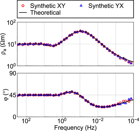
FIGURE 6. The apparent resistivity (ρ_a) and phase (φ) of the synthetic time series of the 1D model obtained by least square method processing.

3D model

The 3D model is closer to the actual situation. To further verify our method, we use the 3D model COMMEMI 3D-2A from (Zhdanov et al., 1997) for the following study. The model background is a three-layer medium (resistivity of 10, 100, and 0.1 Ωm) with two anomalous rectangular bodies (resistivity of 1Ωm and 100Ωm) on the top layer. Eight sites on the model surface were selected to synthesize time series, as shown in Figure 7.

FIGURE 7

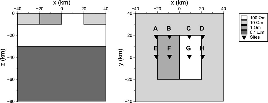
FIGURE 7. Model diagram of COMMEMI 3D-2A, the triangles are the locations of the sites.

The synthetic time series using the same sampling rates as above is shown in Figure 8. For clarity, only a portion of the time series is plotted for each sampling rate. The time series of the horizontal magnetic fields (H_x and H_y) at each site are quite similar, which is similar to the slow spatial variation of the natural horizontal magnetic field. The horizontal electric fields (E_x and E_y) at each site are quite similar in morphology but differ in amplitude and phase. This is because the electric field signal is more easily affected by the electrical structure under the same natural field source. The resistivity below site F is much lower than that at site G, so the horizontal electric field amplitude at site F is always smaller than that at site G with the same source. Consequently, the morphology of the synthetic time series is consistent with the given model.

FIGURE 8

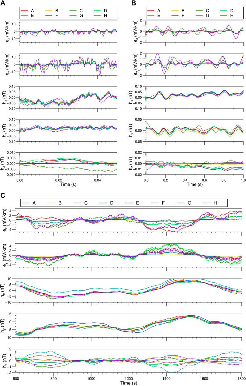
FIGURE 8. Synthetic time series of 8 sites in the 3D model. (A) Time series with 2400Hz sampling rate, (B) Time series with 150Hz sampling rate, (C) Time series with 15Hz sampling rate.

To facilitate processing with existing software, we add the observed system responses to the synthetic time series and output them in MTU-5A format. We processed the time series using the least-squares method, the commercial software SSMT2000 and the open-source software EMTF (Egbert, 1997). Figure 9 shows the processing results. All the results are consistent with the theoretical response, indicating that the synthetic time series of the 3D model are accurate and can be processed by existing methods.

FIGURE 9

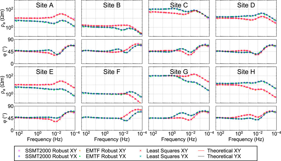
FIGURE 9. The processing results of the synthetic time series of 8 stations in the 3D model.

To further analyze the synthetic time series, we divided the time series into sections (to distinguish the “segment” in synthesizing time series, “section” is used here). Every two adjacent sections overlap by 50%. We preform the Fourier transform on each section, and calculate the frequency domain parameters such as the PSD of the electromagnetic field, the impedance tensor, the tipper vector, the ordinary coherence, and the polarization direction. These parameters were usually used in frequency domain selection techniques for MT noise separation (Weckmann et al., 2005). The PSD is defined as:

$PSD\left(A\right)=\frac{\sqrt{[A{A}^{*}}{]}^2}{\mathrm{\Delta }T},(9)$

where A = E_x(ω), E_y(ω), H_x(ω), H_y(ω) or H_z(ω), ΔT is the length of the section, A* is the complex conjugate of A.

The ordinary coherence is defined as:

$coh\left(AB\right)=\frac{|\left[A{B}^{*}\right]{|}^2}{\left[A{A}^{*}\right]\left[B{B}^{*}\right]},(10)$

where B is the same as A, but can be different field components.

The polarization direction α_E and α_H of electric and magnetic field are:

$\left\{\begin{array}{c}{\alpha }_E=\arctan \frac{2*\mathfrak{R}\left(\left[E_x{E}_y^{*}\right]\right)}{\left[E_x{E}_x^{*}\right]-\left[E_y{E}_y^{*}\right]}\hfill \\ {\alpha }_H=\arctan \frac{2*\mathfrak{R}\left(\left[H_x{H}_y^{*}\right]\right)}{\left[H_x{H}_x^{*}\right]-\left[H_y{H}_y^{*}\right]}\hfill \end{array}\right..(11)$

where $\mathfrak{R}$ stands for the real part.

Figure 10 shows the MT parameters at 2.25 Hz. The PSD distribution of electromagnetic field shows a random variation of signal intensity similar to natural fields. The distribution of the transfer function estimates exhibit one cluster around the actual value. The coherence of the orthogonal electromagnetic field is concentrated near 1. The polarization direction of electric and magnetic fields are disordered with time. The distributions of all these parameters follow those of a low-noise natural-field MT signal, suggesting that the synthetic time series can simulate natural MT signal with a high signal-to-noise.

FIGURE 10

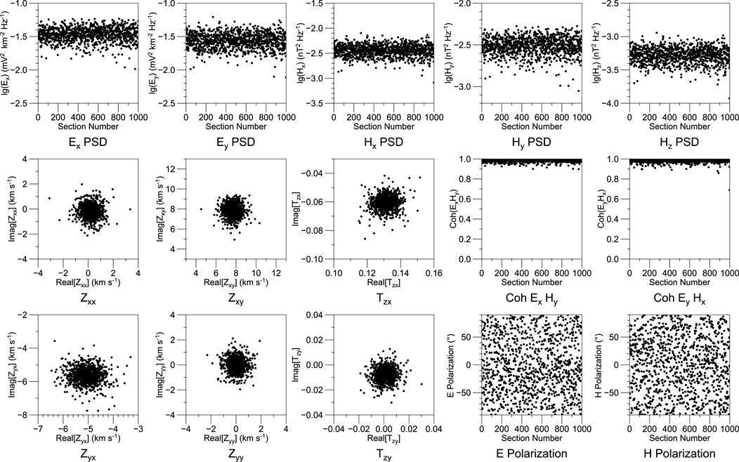
FIGURE 10. The distribution of parameters at 2.25 Hz of synthetic time series of site A. The x-axis of most graphs shows the section numbers. The six response function plots are displayed in the complex plane.

Noise test

By adding noise to the synthetic time series, we can test the effects of various noises on the MT response and verify the denoising ability, estimation results, and robustness of the data processing methods. For example, square-wave, triangular-wave, and impulsive noise are three common types of noise in MT exploration. We generated the three types of noise by pseudo-random, and added them to the E_x channel at site A (Figure 11).

FIGURE 11

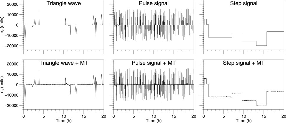
FIGURE 11. Synthetic time series with noise. The duration of the time series is 20 h.

We investigated the effect of different noises on the MT response by processing raw synthetic and noisy time series using the least-squares method. Figure 12 shows the apparent resistivity and phase curves. Different noises affect different frequency ranges. Triangular waves and step noise with large timescales affect low frequencies below 1 Hz. Impulsive noise has no effect on frequencies below 0.01 Hz, but only affects frequencies between 2 Hz and 0.01 Hz in a range similar to the dead band. Different noise has different effects on apparent resistivity and phase curve morphology. The apparent resistivity and phase, the apparent resistivity and phase are irregular in all but the case of triangular wave noise, which causes the apparent resistivity to increase steadily with decreasing frequency.

FIGURE 12

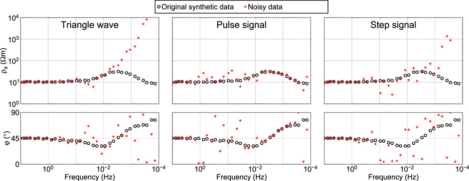
FIGURE 12. Response of time series with noise. Processed by the least-square method.

EMTF and SSMT2000 are the two most commonly used MT time series processing software. SSMT2000 is commonly used in conjunction with the frequency domain data selection software MTEditor to improve estimation quality. We used EMTF and SSMT2000 to process the noisy time series, and use MTEditor to select the spectral data processed by SSMT 2000. The final results are shown in Figure 13. Both EMTF and SSMT2000 provided accurate impedance estimation for synthetic time series with triangular and step noise at frequencies above 0.002 Hz. For low frequencies below 0.002 Hz, accurate impedance estimates were not obtained by either method due to insufficient stacking. For time series with impulsive noise, EMTF was able to accurately estimate the impedance in the frequency band affected by the noise, while SSMT2000 was unable to accurately estimate the impedance in a few frequencies. However, careful selection of spectral data using MTEditor improved the estimation of these frequencies. Moreover, in the low-frequency, the MTEditor result had three or four more effective frequencies than the other two results, so that SSMT2000 combined with MTEditor achieves the best performance in this test.

FIGURE 13

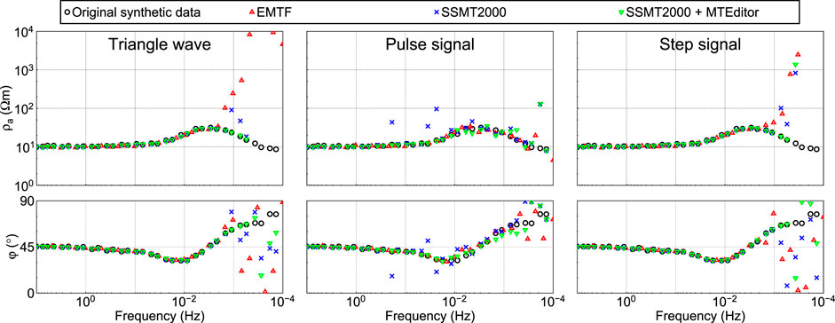
FIGURE 13. Comparison of processing results between EMTF and SSMT 2000. SSMT2000+MTEditor is the result processed by SSMT2000 and by MTEditor.

The above test results show that the synthesized time series of the proposed method can be used not only as the carrier of noise signals to study the influence of different noises on MT response, but also as a test standard to study the processing performance of different data processing methods to specific noises.

Conclusion

We propose a synthetic MT time series method based on forward modeling. First, the electromagnetic response of two orthogonal polarization sources for a given model is calculated using MT forward modeling. Then, the electromagnetic responses of the two polarization sources are randomly combined to simulate the random polarization properties of the natural field sources. Next, the electromagnetic fields are transformed from the frequency domain to the time domain according to the correspondence between the time and frequency domains. Finally, the time-varying source polarization is simulated by segmentation and concatenation to generate time series. We use this method to synthesize time series of 1D and 3D models. The spectral analysis of the synthetic time series shows that the distribution of the parameters in the frequency domain is similar to that of the measured low-noise natural field data. Commercial software and open-source software were used to process the synthetic time series, and the apparent resistivity and phase closely match the forward modeling response of the given model, confirming the correctness of the proposed method. By adding different types of noise into the synthetic time series, the effect of noise on MT response is analyzed, and the performance of different time series processing methods is tested and compared, which proves that the synthetic time series can be used as the evaluation criterion of time series processing methods.

The time series of all channels synthesized by the proposed method are directly derived from MT forward modeling, which is more reasonable than previous techniques that require a pre-determined time series of the magnetic fields. As shown in the 3D model example, time series of complex models can be synthesized to provide an effective study sample for analyzing the spatial distribution and temporal variability of MT time series of specific models. Synthetic time series can be used for single- and multi-site data processing studies. This method can be used to synthesize not only MT time series, but also time series of other frequency-domain electromagnetic methods. Therefore, various artificial source noises can be synthesized and added to the synthetic MT time series to investigate the signal-to-noise separation method, which is also the focus of our future study. Synthetic time series can provide rich and diverse learning samples for deep learning techniques, which can help apply artificial intelligence techniques in MT time series processing.

In summary, the method presented in this paper provides a technical basis to transform the forward modeling of electromagnetic responses from the frequency domain to the time domain. We can obtain time series for any model, which amounts to providing a standard signal generator for the study of time series processing techniques. In addition to testing the effectiveness of the time series processing method, it can be applied to other aspects. For example, to analyze the effect of different types of noise on the MT response, we can synthesize time series containing different noises, and then compare the processing results of noisy time series with the forward modeling response. In a practical MT application, after obtaining the inversion model of the studied region, we can attempt to extract the actual natural source information through time series of low-noise sites. We may then be able to construct random sources that are highly correlated with the true natural sources and synthesize time series for the inversion model. Moreover, time series not derived from the inversion model can be separated to study the distribution of noise. In this way, we can extract the source of the remote reference station and synthesize the time series highly correlated with the observation station, which can be used as the reference channels to improve the quality of the measured data. In other words, many new and interesting studies can be carried out based on the synthetic time series method proposed in this paper.

Data availability statement

The open-source code for the method and the data in the paper are available on Github: https://github.com/EMWPJ/SyntheticMTTimeSeries and https://github.com/EMWPJ/MT-synthetic-time-series-Data.

Author contributions

PW implemented the algorithms and wrote the manuscript. XC came up with the idea of the algorithm, supervised the study, performed the analyses, and edited the manuscript. YZ helped in processing the data and drew the figures.

Funding

This work is supported by the National Natural Science Foundation of China (41941016), the 2nd comprehensive scientific investigation into the Tibetan Plateau (2019QZKK0708), and the National Natural Science Foundation of China (42174093).

Acknowledgments

We are grateful to Anna Kelbert, Naser Meqbel, Gary D. Egbert, and Kush Tandon for providing the ModEM code (Kelbert et al., 2014). Generic Mapping Tools software (Wessel et al., 2019) was used to produce the figures in this manuscript.

Conflict of interest

The authors declare that the research was conducted in the absence of any commercial or financial relationships that could be construed as a potential conflict of interest.

Publisher’s note

All claims expressed in this article are solely those of the authors and do not necessarily represent those of their affiliated organizations, or those of the publisher, the editors and the reviewers. Any product that may be evaluated in this article, or claim that may be made by its manufacturer, is not guaranteed or endorsed by the publisher.

Supplementary material

The Supplementary Material for this article can be found online at: https://www.frontiersin.org/articles/10.3389/feart.2023.1086749/full#supplementary-material

References

Banks, R. J. (1998). The effects of non-stationary noise on electromagnetic response estimates. Geophys. J. Int. 135, 553–563. doi:10.1046/j.1365-246X.1998.00661.x

CrossRef Full Text | Google Scholar

Cai, J., and Chen, Q. (2015). Spectrum analysis of magnetotelluric data series based on EMD-teager transform. Pure Appl. Geophys. 172, 2901–2915. doi:10.1007/s00024-015-1083-0

CrossRef Full Text | Google Scholar

Cai, J., Chen, X., Xu, X., Tang, J., Wang, L., Guo, C., et al. (2017). Rupture mechanism and seismotectonics of the M_s 6.5 Ludian earthquake inferred from three?dimensional magnetotelluric imaging. Geophys. Res. Lett. 44, 1275–1285. doi:10.1002/2016GL071855

CrossRef Full Text | Google Scholar

Cai, J. (2014). A combinatorial filtering method for magnetotelluric time-series based on Hilbert–Huang transform. Explor. Geophys. 45, 63–73. doi:10.1071/EG13012

CrossRef Full Text | Google Scholar

Campanya, J., Ledo, J., Queralt, P., Marcuello, A., and Jones, A. G. (2014). A new methodology to estimate magnetotelluric (mt) tensor relationships: Estimation of local transfer-functions by combining interstation transfer-functions (elicit). Geophys. J. Int. 198, 484–494. doi:10.1093/gji/ggu147

CrossRef Full Text | Google Scholar

Carbonari, R., D’Auria, L., Di Maio, R., and Petrillo, Z. (2017). Denoising of magnetotelluric signals by polarization analysis in the discrete wavelet domain. Comput. Geosciences 100, 135–141. doi:10.1016/j.cageo.2016.12.011

CrossRef Full Text | Google Scholar

Chave, A. D., and Thomson, D. J. (2004). Bounded influence magnetotelluric response function estimation. Geophys. J. Int. 157, 988–1006. doi:10.1111/j.1365-246X.2004.02203.x

CrossRef Full Text | Google Scholar

Chave, A. D., Thomson, D. J., and Ander, M. E. (1987). On the robust estimation of power spectra, coherences, and transfer functions. J. Geophys. Res. 92, 633. doi:10.1029/JB092iB01p00633

CrossRef Full Text | Google Scholar

Chave, A. D. (2014). Magnetotelluric data, stable distributions and impropriety: An existential combination. Geophys. J. Int. 198, 622–636. doi:10.1093/gji/ggu121

CrossRef Full Text | Google Scholar

Chave, A. D. (2017). Estimation of the magnetotelluric response function: The path from robust estimation to a stable maximum likelihood estimator. Surv. Geophys. 38, 837–867. doi:10.1007/s10712-017-9422-6

CrossRef Full Text | Google Scholar

Egbert, G. D., and Booker, J. R. (1986). Robust estimation of geomagnetic transfer functions. Geophys. J. Int. 87, 173–194. doi:10.1111/j.1365-246X.1986.tb04552.x

CrossRef Full Text | Google Scholar

Egbert, G. D. (1997). Robust multiple-station magnetotelluric data processing. Geophys. J. Int. 130, 475–496. doi:10.1111/j.1365-246X.1997.tb05663.x

CrossRef Full Text | Google Scholar

Escalas, M., Queralt, P., Ledo, J., and Marcuello, A. (2013). Polarisation analysis of magnetotelluric time series using a wavelet-based scheme: A method for detection and characterisation of cultural noise sources. Phys. Earth Planet. Interiors 218, 31–50. doi:10.1016/j.pepi.2013.02.006

CrossRef Full Text | Google Scholar

Gamble, T. D., Goubau, W. M., and Clarke, J. (1979a). Error analysis for remote reference magnetotellurics. Geophysics 44, 959–968. doi:10.1190/1.1440988

CrossRef Full Text | Google Scholar

Gamble, T. D., Goubau, W. M., and Clarke, J. (1979b). Magnetotellurics with a remote magnetic reference. Geophysics 44, 53–68. doi:10.1190/1.1440923

CrossRef Full Text | Google Scholar

Goubau, W. M., Gamble, T. D., and Clarke, J. (1978). Magnetotelluric data analysis: Removal of bias. Geophysics 43, 1157–1166. doi:10.1190/1.1440885

CrossRef Full Text | Google Scholar

Guo, Z., Han, J., Gong, X., Liu, L., Zhou, R., and Wu, Y. (2022). ADMM-based method for estimating magnetotelluric impedance in the time domain. IEEE Trans. Geoscience Remote Sens. 60, 1–16. doi:10.1109/TGRS.2022.3171768

CrossRef Full Text | Google Scholar

Jiang, F., Chen, X., Unsworth, M. J., Cai, J., Han, B., Wang, L., et al. (2022). Mechanism for the uplift of gongga Shan in the southeastern Tibetan plateau constrained by 3d magnetotelluric data. Geophys. Res. Lett. 49, e2021GL097394. doi:10.1029/2021GL097394

CrossRef Full Text | Google Scholar

Junge, A. (1996). Characterization of and correction for cultural noise. Surv. Geophys. 17, 361–391. doi:10.1007/BF01901639

CrossRef Full Text | Google Scholar

Kappler, K. N. (2012). A data variance technique for automated despiking of magnetotelluric data with a remote reference: MT data despiking. Geophys. Prospect. 60, 179–191. doi:10.1111/j.1365-2478.2011.00965.x

CrossRef Full Text | Google Scholar

Kelbert, A., Meqbel, N., Egbert, G. D., and Tandon, K. (2014). ModEM: A modular system for inversion of electromagnetic geophysical data. Comput. Geosciences 66, 40–53. doi:10.1016/j.cageo.2014.01.010

CrossRef Full Text | Google Scholar

Kelbert, A., Balch, C. C., Pulkkinen, A., Egbert, G. D., Love, J. J., Rigler, E. J., et al. (2017). Methodology for time-domain estimation of storm time geoelectric fields using the 3-d magnetotelluric response tensors. Space weather. 15, 874–894. doi:10.1002/2017SW001594

CrossRef Full Text | Google Scholar

Larsen, J. C., Mackie, R. L., Manzella, A., Fiordelisi, A., and Rieven, S. (1996). Robust smooth magnetotelluric transfer functions. Geophys. J. Int. 124, 801–819. doi:10.1111/j.1365-246X.1996.tb05639.x

CrossRef Full Text | Google Scholar

Li, G., Liu, X., Tang, J., Deng, J., Hu, S., Zhou, C., et al. (2020a). Improved shift-invariant sparse coding for noise attenuation of magnetotelluric data. Earth, Planets Space 72, 45. doi:10.1186/s40623-020-01173-7

CrossRef Full Text | Google Scholar

Li, G., Liu, X., Tang, J., Li, J., Ren, Z., and Chen, C. (2020b). De-noising low-frequency magnetotelluric data using mathematical morphology filtering and sparse representation. J. Appl. Geophys. 172, 103919. doi:10.1016/j.jappgeo.2019.103919

CrossRef Full Text | Google Scholar

Li, G., Li, J., Liu, X., and Tang, J. (2020c). Magnetotelluric noise suppression based on impulsive atoms and NPSO-omp algorithm. Pure Appl. Geophys. 177, 5275–5297. doi:10.1007/s00024-020-02592-z

CrossRef Full Text | Google Scholar

Loddo, M., Schiavone, D., and Siniscalchi, A. (2002). Generation of synthetic wide-band electromagnetic time series. Ann. Geophys. 45, 289–301. doi:10.4401/ag-3506

CrossRef Full Text | Google Scholar

Pomposiello, M. C., Booker, J. R., and Favetto, A. (2009). A discussion of bias in magnetotelluric responses. Geophysics 74, F59–F65. doi:10.1190/1.3147132

CrossRef Full Text | Google Scholar

Shalivahan, , and Bhattacharya, B. B. (2002). How remote can the far remote reference site for magnetotelluric measurements be? J. Geophys. Res. Solid Earth 107, 2105. doi:10.1029/2000JB000119

CrossRef Full Text | Google Scholar

Sims, W. E., Bostick, F. X., and Smith, H. W. (1971). The estimation of magnetotelluric impedance tensor elements from measured data. Geophysics 36, 938–942. doi:10.1190/1.1440225

CrossRef Full Text | Google Scholar

Smirnov, M. Y. (2003). Magnetotelluric data processing with a robust statistical procedure having a high breakdown point. Geophys. J. Int. 152, 1–7. doi:10.1046/j.1365-246X.2003.01733.x

CrossRef Full Text | Google Scholar

Sutarno, D. (2005). Development of robust magnetotelluric impedance estimation: A riview. Indonesian J. Phys. 16, 79–89.

Google Scholar

Szarka, L. (1988). Geophysical aspects of man-made electromagnetic noise in the Earth—a review. Surv. Geophys. 9, 287–318. doi:10.1007/BF01901627

CrossRef Full Text | Google Scholar

Varentsov, I., and Sokolova, E. Y. (1995). Generation of synthetic magnetotelluric data. Izvestiya Phys. Solid Earth 30, 554–562.

Google Scholar

Wang, H., Campanyà, J., Cheng, J., Zhu, G., Wei, W., Jin, S., et al. (2017). Synthesis of natural electric and magnetic time-series using inter-station transfer functions and time-series from a neighboring site (stin): Applications for processing mt data. J. Geophys. Res. Solid Earth 122, 5835–5851. doi:10.1002/2017JB014190

CrossRef Full Text | Google Scholar

Wang, B., Liu, J., Hu, X., Liu, J., Guo, Z., and Xiao, J. (2021). Geophysical electromagnetic modeling and evaluation: A review. J. Appl. Geophys. 194, 104438. doi:10.1016/j.jappgeo.2021.104438

CrossRef Full Text | Google Scholar

Weckmann, U., Magunia, A., and Ritter, O. (2005). Effective noise separation for magnetotelluric single site data processing using a frequency domain selection scheme. Geophys. J. Int. 161, 635–652. doi:10.1111/j.1365-246X.2005.02621.x

CrossRef Full Text | Google Scholar

Wessel, P., Luis, J. F., Uieda, L., Scharroo, R., Wobbe, F., Smith, W. H. F., et al. (2019). The generic mapping Tools version 6. Geochem. Geophys. Geosystems 20, 5556–5564. doi:10.1029/2019GC008515

CrossRef Full Text | Google Scholar

Zhang, Y., Wang, P., Chen, X., Zhan, Y., Han, B., Wang, L., et al. (2022). Magnetotelluric time series processing in strong inferference environment. Seismol. Geol. 44, 786. doi:10.3969/j.issn.0253-4967.2022.03.014

CrossRef Full Text | Google Scholar

Zhdanov, M., Varentsov, I., Weaver, J., Golubev, N., and Krylov, V. (1997). Methods for modelling electromagnetic fields results from COMMEMI—The international project on the comparison of modelling methods for electromagnetic induction. J. Appl. Geophys. 37, 133–271. doi:10.1016/S0926-9851(97)00013-X

CrossRef Full Text | Google Scholar

Zhou, R., Han, J., Li, T., and Guo, Z. (2022). Fast independent component analysis denoising for magnetotelluric data based on a correlation coefficient and fast iterative shrinkage threshold algorithm. IEEE Trans. Geoscience Remote Sens. 60, 1–15. doi:10.1109/TGRS.2022.3182504

CrossRef Full Text | Google Scholar