Correction method by introducing cloud cover forecast factor in model temperature forecast

1 Introduction

In recent years, with the advancement of numerical forecast and the continuous improvement of statistical methods such as model output statistics (MOS), perfect prognosis (PP), artificial neural networks (ANN), Kalman filter (KF), and the support vector machine (SVM) (Huang and Xie, 1993; Zhang and Sha, 2001; Wang et al., 2004; Chen et al., 2005; Wu et al., 2007; Qian et al., 2010; Chen et al., 2011; Li et al., 2011), the accuracy of temperature forecasts has been greatly improved, but it is still unable to meet people’s growing demand for accurate and refined temperature forecasts. Therefore, methods of improving the accuracy of forecasts is an urgent issue. Temperature is sensitive to local weather and geographical characteristics. The MOS is the most commonly method used in daily temperature forecasting. It can introduce many forecast factors that are difficult to introduce by other methods, match local weather and climate characteristics, and make appropriate corrections to the systematic deviations of numerical models (Liu et al., 2004).

The MOS forecast method usually requires a certain length of historical data samples to achieve better forecast results. The samples should preferably have the same climate background characteristics, and the consistency factors of the samples should be as large as possible. Che et al. (2011) used the K-mean clustering method to make seasonal divisions in North China for temperature forecasts; the forecast error is generally smaller than the traditional seasonal division. Zhi et al. (2010, 2014) compared the different training periods of super-ensemble temperature forecasts and found that a sliding training period is better than a fixed training period. Wu et al. (2016) further optimized the division method of the training period. They used the quasi-symmetric sliding training period method to revise the model temperature forecast by selecting the sample data 1 month before and after the forecast date and also considered the model consistency and the sample’s climate characteristics, which significantly improved the forecast quality. However, methods that highlight the training period do not consider the influencing factor of temperature. Many scholars in China have introduced multiple factors. Liu et al. (2004) selected multiple factors for MOS forecasts, and the forecast verification results showed that the short-term temperature forecast was improved in most cases. Zhang et al. (2011) used the MOS method to select 11 factors on the basis of T213 to forecast the daily maximum and minimum temperatures of 124 stations in Yunnan Province, and the forecast results were improved, especially in summer. Zhu and Mu (2013) established a MOS forecast equation based on the WRF model, using temperature, wind, sea level pressure, relative humidity, and precipitation at Urumqi Airport as forecast factors. The accuracy of the hourly temperature forecast was significantly improved compared with the forecast results directly output by the model. The introduction of multiple factors to establish equations can improve temperature prediction, but the factors should be selected to optimize the role of the main factors.

The local variation of temperature depends on temperature advection, pressure change, atmospheric stability, and diabatic processes (Zhu et al., 2000). Liang and Huang (2006) pointed out that in the absence of large-scale system transit, the diabatic processes are the main factors that affect the temperature change in the near-surface layer, while the diabatic processes are affected by many factors, such as the sky condition, the topography, underlying surface, and vegetation type. Therefore, it is necessary to fully consider the role of cloud cover in temperature forecast. Qin et al. (2007) analyzed the relationship between cloud cover and temperature in Nanning City and found that total cloud cover has a significant negative correlation with mean temperature and maximum temperature, while low cloud cover has a significant negative correlation with maximum temperature and a significant positive correlation with minimum temperature. Zheng et al. (2013) adopted the optimized cloud scheme in GRAPES, and the surface temperature simulated by the model was closer to the observed value. Luo et al. (2014) classified the sky conditions and established the classic MOS forecast model. They selected the numerical forecast product factors corresponding to the general occurrence time of maximum and minimum temperature, which positively and significantly improved the quality of local temperature forecast. Forecasters also make adjustments to temperature forecasts by evaluating the cloud cover in practice, but the specific adjustment extent varies from person to person and cannot be uniformly regulated.

Currently, most MOS temperature forecast methods directly perform one-dimensional regression correction on the model temperature forecast product, which can achieve good correction effects. The forecast quality is not worse than that of multi-factor modeling correction and has been widely used in many meteorological departments. Different amounts of cloud cover will cause differences in the deviation between the model temperature forecast and the actual observation. Therefore, it is meaningful to introduce cloud cover forecast as an auxiliary factor to further optimize the MOS temperature forecast, but few people have studied and applied it in practice. The Fujian Provincial Meteorological Observatory divided temperature samples according to different total cloud cover, established independent models for each subset, and achieved good correction effects. It ranked first in the comprehensive skill of temperature in the 2021 National Meteorological System Intelligent Forecast Technology Method Exchange Competition. In this paper, the optimal scheme of daily maximum and daily minimum temperature forecasts based on cloud cover is selected by further studying the cloud cover groupings and comparing several schemes.

2 Data and pre-processing

2.1 Data

In this paper, the maximum and minimum temperature at 2 m, total cloud cover, and low cloud cover of ECMWF from 2018 to 2021 issued by the China Meteorological Administration were adopted. The ECMWF data are obtained twice a day at 08:00 and 20:00 (Beijing time, same below), and the forecast time period is 0–240 h, the horizontal resolution is 0.125° × 0.125°, and the time resolution is 3 h for 0–72 h and 6 h for 78–240 h. To ensure calculation efficiency and reliability of the observation data, the testing stations are 70 national meteorological stations in Fujian Province.

2.2 Data pre-processing

The inverse distance weighting interpolation method is used to interpolate the ECMWF fine grid point surface elements to the station, and the Cressman objective interpolation method is used as a reference for the weighting coefficients. This is carried out for station-based modeling and forecast. The interpolation method is as follows:

${\mathrm{P}}_{\mathrm{k}}=\frac{{\displaystyle \sum _{\mathrm{i}=1}^{\mathrm{m}}}{\displaystyle \sum _{\mathrm{j}=1}^{\mathrm{n}}}{\mathrm{W}}_{\mathrm{k}\mathrm{i}\mathrm{j}}{\mathrm{P}}_{\mathrm{i}\mathrm{j}}}{{\displaystyle \sum _{\mathrm{i}=1}^{\mathrm{m}}}{\displaystyle \sum _{\mathrm{j}=1}^{\mathrm{n}}}{\mathrm{W}}_{\mathrm{k}\mathrm{i}\mathrm{j}}}(1)$

In Formula 1, P_k is the forecast value of the element at the kth station obtained by interpolation, P_ij is the forecast value of the element at the grid point (i, j), W_kij is the weight factor, and m and n are the numbers of grid points in the latitudinal and longitudinal directions, respectively. The weighting factor used in this paper can be expressed as follows:

$W_{kij}=\left\{\begin{array}{l}\frac{R^2-d_{kij}^2}{R^2+d_{kij}^2},d_{kij}<R\\ 0,d_{kij}\ge R\end{array}\right.(2)$

In Formula 2, R is the effective influence radius and d_kij is the distance from grid point (i, j) to station k. In operational work, for the convenience of calculation, the difference between longitude and latitude is used to represent the distance, and the effective influence radius is taken as 1°.

The daily maximum temperature (T_max) and the daily minimum temperature (T_min) are calculated as the maximum and minimum temperatures over a 24-h period, respectively. Cloud cover (total cloud cover or low cloud cover) is calculated as the 12-h mean cloud cover, and the mean cloud cover at a given point is the mean of all available cloud cover forecasts at that point within a given forecast time period. Because the latest ECMWF data are usually obtained later than the forecast start time, the forecast in this paper is the correction of the model lag of 12 h; that is, the first day of operational forecast corresponds to the 12–36-h period of the model forecast and so on for the other forecast periods.

3 Methods

3.1 Correction method

The one-dimensional linear regression equations for T_max and T_min at a certain forecast period for each station are established using the least square method:

$S_i=a+b{F}_i.(3)$

In Formula 3, $S_i$ is regression correction temperature at the ith forecast period, $F_i$ is the temperature forecast value of the model at this period, a is a constant, and b is the regression coefficient. Taking cloud cover as the division basis, the forecast value and observation value are used to establish a and b for each subset after division and are updated twice a day, and the obtained regression equation is used to correct T_max and T_min of the corresponding subset.

During the day, direct solar radiation can reach the earth’s surface and warm it. If there is cloud cover, the cloud layer will reflect some of the solar radiation, reducing the energy input to the surface and hindering warming. At night, the heat released from the surface dissipates upwards, causing the surface temperature to decrease. If there is cloud cover, the cloud layer can reflect the heat from the surface, thereby weakening heat dissipation and hindering cooling. Therefore, the effect of cloud cover on surface temperature is opposite during the day and night, and the reverse is true under clear skies. Because cloud cover at night and during the day has opposite effects on temperature, daytime cloud cover is used as the auxiliary factor for the correction of T_max, and nighttime cloud cover is used as the auxiliary factor for correction of T_min.

3.2 Training period

The quasi-symmetric mixed sliding training period method can significantly improve the quality of a temperature forecast by the MOS method and has great application value in operational work (Wu et al., 2016). This paper continues to use this method, and the total samples during the training period mixed samples from 35 days before the forecast date and samples from 35 days after the forecast day of the previous year and used sliding sampling with the forecast date.

3.3 Inspection method

To evaluate the operational performance of the MOS forecast, the mean absolute error of temperature forecast (MAE, Zhou et al., 2006), the temperature forecast accuracy (FA), and the temperature forecast skill scores (FSS) were used in this paper:

$FA=\frac{N_r}{N_f}\times 100\%.(4)$

In Formula 4, FA is the percentage of the absolute deviation between the temperature forecast whose observed value does not exceed 2°C, N_r is the number of stations (times) where the value of the difference between the forecast temperature and the observed value does not exceed 2°C, and N_f is the total number of stations (times) that have been forecasted.

$FSS=\frac{{MAE}_0-{MAE}_N}{{MAE}_0}(5)$

In Formula 5, ${MAE}_O$ is the MAE of the temperature forecast of the initial scheme and ${MAE}_{\mathrm{N}}$ is the MAE of the temperature forecast for the improved scheme. When ${MAE}_O=0$, FSS = 1.01.

4 Scheme comparison and improvement

4.1 Initial scheme design

Based on the observed temperature data from 2019 to 2020 and temperature, total cloud cover, and low cloud cover forecast data from ECMWF, three schemes are designed and compared to discuss the feasibility and the improvement direction of introducing cloud cover.

Scheme 1: No grouping, using the quasi-symmetric mixed sliding training period method (one-dimensional regression) to model and revise all temperature forecast samples (Wu et al., 2016).

Scheme 2: Grouping by total cloud cover, the temperature forecast samples with total cloud cover less than the specified threshold value are grouped for separate modeling correction, and the remaining samples are grouped as another group. The exhaustive method is used for the cloud cover threshold, starting from 0% total cloud cover as the threshold, increasing to 100% at 5% intervals; 21 cloud cover values were selected as grouping thresholds for correction.

Scheme 3: Grouping by low cloud cover, the temperature forecast samples with cloud cover less than the specified threshold are grouped for separate modeling correction, and the remaining samples are grouped as another group. Groupings of the cloud thresholds are the same as in Scheme 2.

According to the forecast results of Scheme 2 (Figure 1A), the absolute forecast deviation of T_max for the first day is less than that of no grouping (the threshold of 0% cloud cover can be approximated to no grouping). When about 30%–40% cloud cover is used as the grouping threshold, the forecast result is better, the MAE is small, and the MAE of the optimal threshold can be reduced by about 0.05°C. For the T_min forecast (Figure 1B), the MAE of grouping is also less than that of no grouping. The improvement is obvious when grouping by the less and more cloud cover threshold intervals, and grouping by the less cloud cover threshold is slightly better than grouping by the more cloud cover threshold. Because the potential for improvement of the T_min forecast is smaller than that of the T_max forecast, there is not much difference between the different thresholds. The performance of Scheme 3 is similar to that of Scheme 2 and will not be presented separately.

FIGURE 1

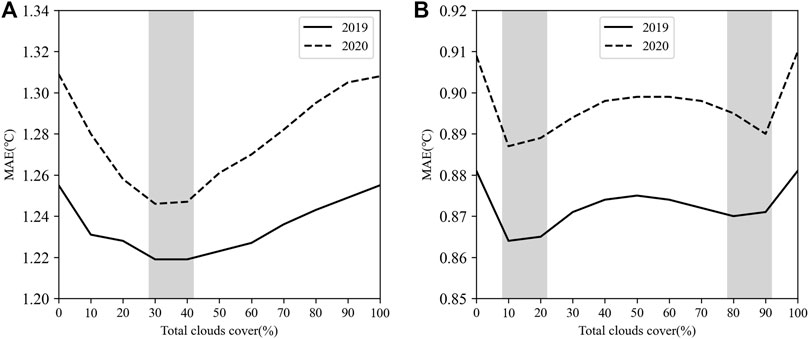
FIGURE 1. Comparison of the MAE of different total cloud cover threshold forecasts on the first day. (A) T_max; (B) T_min.

The optimal threshold scheme of T_max and T_min among the 21 grouping methods of Scheme 2 and Scheme 3 was selected to compare with Scheme 1 and the original uncorrected results. The results are shown in Figure 2. Seen from FA, the forecast results of T_max and T_min in all three revised schemes were significantly improved compared with the original uncorrected ones, and the improvement rate in the first 5 days was 100% or above. For T_max, the scheme grouping by total cloud cover performed better than the other two schemes in all forecast periods in terms of FA and MAE (Figures 2A, C). The FA of the scheme grouping by low cloud cover improved compared with no grouping in the first 4 days, but it was not better on the fifth day, while the MAE improved in all time periods. For T_min, the performance of Scheme 2 was also the best compared with the other schemes in all forecast periods (Figures 2B, D), followed by Scheme 3, and both schemes were better than Scheme 1 in terms of FA and MAE. In general, the introduction of cloud cover improved the forecast performance, and the introduction of total cloud cover was better than low cloud cover.

FIGURE 2

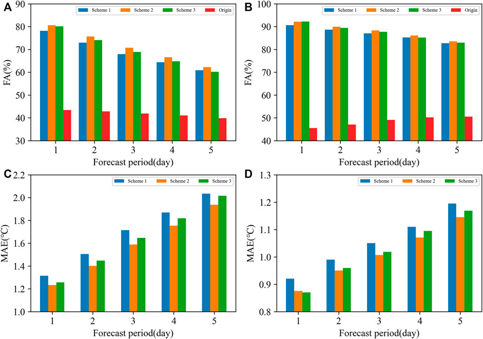
FIGURE 2. Comparison of the forecast results of the three schemes from 2019 to 2020. (A) FA of T_max (unit: %), (B) FA of T_min (unit: %), (C) MAE of T_max (unit: °C), and (D) MAE of T_min (unit: °C).

4.2 Relationship between cloud cover and temperature correction forecast deviation

In general, the least squares method is used to directly model and correct based on the modeled temperature forecast products. The ideal result of the mean deviation of the objective temperature forecast is unbiased; however, there is a significant correlation between forecast deviation of temperature and cloud cover. Figure 3 shows the relationship between the mean forecast deviation of T_max and T_min based on Scheme 1 and the total cloud cover with a 12–36 h forecast period in 2019 and 2020 for 70 national meteorological stations. The relationship between low cloud cover and temperature forecast is similar to the total cloud cover, which is not given in the paper. It can be seen that for T_max (Figure 3A), the 2-year mean forecast deviation of temperature has a good positive linear correlation with cloud cover; the correlation coefficient is 0.85 in 2019 and 0.95 in 2020. The forecast value is often less than the actual when the cloud cover is below 30%–40% and has a large linear slope. The forecast tends to be greater than the actual when the cloud cover is above 40% and has a smaller slope. For T_min (Figure 3B), a negative correlation exists below the threshold of 40% cloud cover, with a steep linear slope; the correlation coefficients were −0.96 in 2019 and −0.89 in 2020. Conversely, a positive correlation with a smaller linear slope was found above the threshold of 40% cloud cover; the correlation coefficients were 0.95 in 2019 and 0.96 in 2020. The common point of T_max and T_min is that the absolute deviation will be larger when the cloud cover is low. Although the influence of cloud cover has been considered in the ECMWF temperature forecast, there is still a strong mean correlation between the mean forecast deviation and cloud cover. Meanwhile, schemes of grouping by cloud cover demonstrate an improvement in forecast accuracy. Therefore, the multiple regression scheme introduces a cloud cover factor based on cloud cover grouping that can be used in professional work. In the following, schemes will be designed and compared to select the best.

FIGURE 3

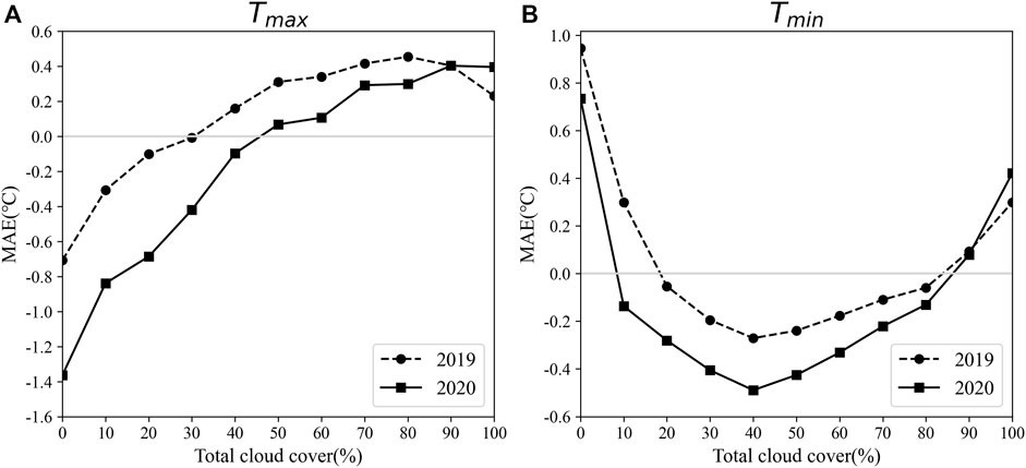
FIGURE 3. Relationship between the mean deviations of 12–36 h forecasts of temperature and the total cloud cover in 2019 and 2020. (A): T_max and (B): T_min.

4.3 Improving scheme design

Based on the aforementioned discussion, improvement plans were designed to maximize forecast performance by considering the roles of total cloud cover, grouping methods, and binary regression methods in the forecast.

Scheme 4: Binary regression, using the quasi-symmetric mixed sliding training period method (Wu et al., 2016), taking temperature and total cloud cover forecast as two forecast factors to establish the forecast equation.

Scheme 5: After grouping by total cloud cover, correction is performed using Scheme 4. From Figure 1A, it can be seen that the optimal threshold for the high-temperature grouping is at 30%–40% cloud cover, and Figure 3 shows that the 40% cloud cover is a special turning point in both T_max and T_min forecasts. In practical applications, less cloud cover is conducive to the increase of daytime T_max and the decrease of nighttime T_min. Therefore, the 40% cloud cover is used as the grouping threshold. After grouping, the cloud cover is introduced for binary regression to establish the forecast equation.

Using the aforementioned two plans, a verification experiment was conducted for T_max and T_min from 2019 to 2020, and the results were compared with Scheme 2 whose grouping threshold is set at 40% cloud cover (Figure 4). In terms of forecast verification results, for T_max (Figures 4A, C), the FA in Scheme 5 is generally larger than that in Scheme 2. With increased forecast time, the improvement is more obvious, but it is slightly less than that of Scheme 4 on the third to fifth days, while Scheme 4 is slightly worse than Scheme 2 on the 1st day. In terms of MAE, Scheme 5 has a slight decrease, which is better than the other two schemes. For T_min (Figures 4B, D), the overall improvement of Scheme 5 is more significant than that of T_max, and all forecast indicators at all forecast periods are improved compared with other schemes. Scheme 3 is better than Scheme 4. In general, Scheme 5 is superior to other schemes. For T_max, there is a linear relationship between the mean forecast deviation and cloud cover, with different slopes between low cloud cover and high cloud cover. Each of the three schemes has advantages, but the performance of the binary regression scheme after grouping performs more stably in terms of MAE. For T_min, the mean forecast deviation has an opposite relationship between less and more cloud cover. Therefore, the binary regression scheme after grouping can better improve the forecast quality.

FIGURE 4

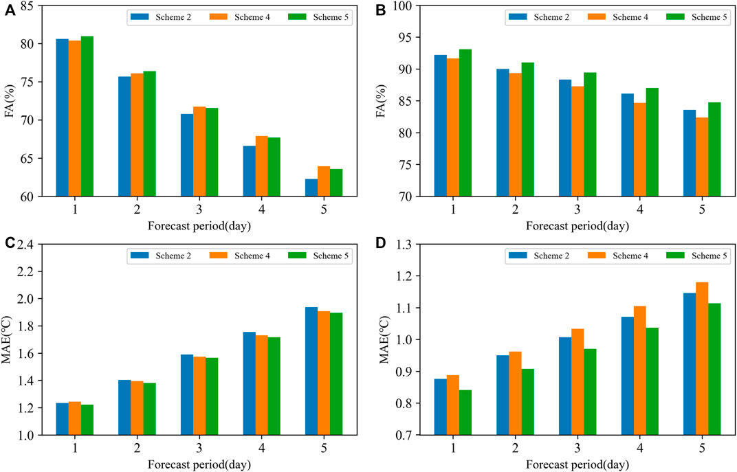
FIGURE 4. Comparison of the forecast results of the three schemes from 2019 to 2020. (A) FA of T_max (unit: %), (B) FA of T_min (unit: %), (C) MAE of T_max (unit: °C), and (D) MAE of T_min (unit: °C).

4.4 Availability and stability of improvement schemes

Scheme 5 was used for temperature forecast in 2021 to test the usability and stability of the method, and the verification results are shown in Table 1. According to the results of the T_max forecast, all verification indicators in Scheme 5 show significant improvements compared to Scheme 1, with an overall increase in FA of 1.2–2.6%. The highest increase is 2.6% on the 1st day; after the improvement, the mean accuracy rate reached 81%. The accuracy continued to increase by about 2% in the fifth to sixth days. MAE decreased by 0.04–0.08°C on all forecast periods, except for slightly less on the 7th day. The first 3 days decreased by about 0.08°C, and the FSS can reach 0.05–0.06. In terms of the T_min forecast, all indicators of all forecast periods also showed improvement, with an increase of 1.0%–2.4% in FA, and the highest increase was 2.36% on the first day. MAE decreased by approximately 0.05°C–0.08°C. The FSS in the first 3 days reached 0.06 to 0.08, and the FA on the first day reached 91.48%.

TABLE 1

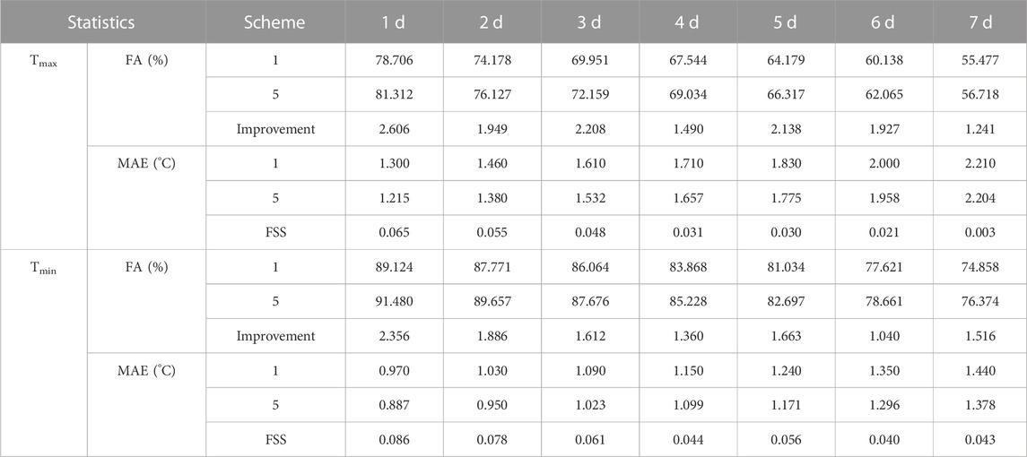
TABLE 1. Test results of T_max and T_min forecasts at 1–7 d by Scheme 1 and Scheme 5 in 2021.

In recent years, the application of the quasi-symmetric sliding training period MOS forecast method has greatly improved T_max and T_min forecast results in Fujian Province. The method ranks among the top in national forecast quality inspections; especially, the FA of T_min is basically more than 90%. Under the condition that the forecast accuracy of the original model has not been improved, there is some room for improvement of the forecast results, but the forecast accuracy of Scheme 5 increased by about 2% compared with Scheme 2 in T_max and T_min forecast in 2021. These findings show that this method can further improve the forecast quality, and it has a certain stability. At present, it has achieved good results in the operational application of actual temperature forecasts in Fujian. Although Scheme 5 showed some improvement in T_max forecasts compared to Scheme 4, the difference was not significant, and the best plan should be selected based on local conditions and corresponding evaluations in practical applications.

5 Conclusion

This paper designs a MOS forecast method that uses total cloud cover as a predictor for the 2 m temperature forecast. Different schemes are designed and optimized using multiple verification indicators. The results show that:

1. All grouping schemes based on cloud cover show improvement in forecast performance, and the introduction of total cloud cover shows advantages over low cloud cover.

2. There is a good positive correlation between the annual mean forecast deviation of the T_max and the mean total cloud cover. For T_min, there is a negative correlation below 40% cloud cover and a positive correlation above it. Both T_max and T_min forecasts have larger absolute deviations when total cloud cover is less than 40%.

3. Whether for T_max or T_min forecast, the binary regression scheme after grouping consistently showed the best performance, with the lowest MAE.

4. Based on the optimization of the scheme in the last 2 years, the improved scheme is used to forecast the T_max and T_min in 2021. The verification indicators show certain improvements in most forecast periods, with FA for T_max and T_min being 81.312% and 91.480%, respectively, which is an improvement of 2.4%–2.6% relative to single-factor regression plans. The FSS of 0.065 for T_max and 0.086 for T_min indicate that this method effectively improves forecast quality and stability, making it suitable for practical forecasting. The introduction of total cloud cover to the MOS forecast can significantly improve the forecast quality, but the correction effect may be poor when the model’s cloud cover forecast has large biases from observations. Further research is needed to determine the reliability of cloud cover forecasts from multiple models and ensemble prediction products.

Data availability statement

The raw data supporting the conclusion of this article will be made available by the authors, without undue reservation.

Author contributions

HM: methodology and writing. WQ: data curation and software. LH: visualization. YS: editing and translation. WG: validation.

Funding

This work was supported by the Natural Science and Technology Program of Fujian Province (2021J01457), the National Key R&D Program (2018YFC1506905), and the Innovation Project of the China Meteorological Administration (CXFZ2021Z009). The Chinese Meteorological Administration’s retrospective summary project (FPZJ2023-061).

Conflict of interest

The authors declare that the research was conducted in the absence of any commercial or financial relationships that could be construed as a potential conflict of interest.

Publisher’s note

All claims expressed in this article are solely those of the authors and do not necessarily represent those of their affiliated organizations, or those of the publisher, the editors, and the reviewers. Any product that may be evaluated in this article, or claim that may be made by its manufacturer, is not guaranteed or endorsed by the publisher.

References

Che, Q., Zhao, S., and Fan, G. (2011). Seasonal partition problem of MOS forecast for extreme temperature in North China[J]. J. Of Appl. Meteorological Sci. 22 (4), 429–436. doi:10.11898/1001-7313.20110405

CrossRef Full Text | Google Scholar

Chen, F., Jiao, M., and Chen, J. (2011). A new scheme calibration of ensemble forecast products based on bayesian processor of output and its study results for temperature prediction [J]. Meteorol. Mon. 37 (1), 14–20. doi:10.7519/j.issn.1000-0526.2011.1.002

CrossRef Full Text | Google Scholar

Chen, Y., Chen, X., Ma, J., and Wen, L. P. (2005). Nano neodymium oxide induces massive vacuolization and autophagic cell death in non-small cell lung cancer NCI-H460 cells. J. Arid Meteorology 23 (4), 52–60. doi:10.1016/j.bbrc.2005.09.018

PubMed Abstract | CrossRef Full Text | Google Scholar

Huang, J., and Xie, Z. (1993). The application of kalman filter technique to weather forecast[J]. Meteorol. Mon. 21 (2), 3–7. doi:10.7519/j.issn.1000-0526.1994.9.009

CrossRef Full Text | Google Scholar

Li, Q., Hu, B., and Wang, X. (2011). Analysis of hail disasters in the central region of gansu Province[J]. J. Arid Meteorology 29 (2), 231–235. doi:10.3969/j.issn.1006-7639.2011.02.017

CrossRef Full Text | Google Scholar

Liang, L., and Huang, G. (2006). Research on forecast method of maximum and minimum temperature at single station[J]. J. Of Guangxi Meteorology 27 (3), 4–6.

Google Scholar

Liu, H., Zhao, S., and Lu, Z. (2004). Objective element forecast at nmc—MOS system[J]. Xin Jiang Meteorol. 27 (3), 4–7.

Google Scholar

Luo, J., Zhou, J., and Yan, Y. (2014). Local temperature MOS forecast method based on numerical forecast products and superior guidance[J]. Meteorological Sci. Technol. 42 (003), 443–450. doi:10.3969/j.issn.1671-6345.2014.03.015

CrossRef Full Text | Google Scholar

Qian, L., Lan, X., and Yang, Y. (2010). The application of optimal subset neural network to temperature objective forecast in wuwei[J]. Meteorol. Mon. 36 (5), 102–107. doi:10.7519/j.issn.1000-0526.2010.5.015

CrossRef Full Text | Google Scholar

Qin, W., Huang, D., and Liao, X. (2007). Analysis of the variation characteristics of cloudiness in nanning and relationship with temperature and precipitation[J]. J. Of Meteorlogical Res. Appl. 28 (4), 14–19.

Google Scholar

Wang, X., Yang, X., and Shi, D. (2004). Application of numerical forecast products to summer high temperature prediction[J]. Meteorological Sci. Technol. 32 (S1), 47–49. doi:10.3969/j.issn.1671-6345.2004.z1.012

CrossRef Full Text | Google Scholar

Wu, J., Pei, H., and Shi, Y. (2007). The forecast of surface air temperature using BP-MOS method based on the numerical forecast results [J]. Sci. Meteorol. Sin. 27 (4), 430–435. doi:10.3969/j.issn.1009-0827.2007.04.012

CrossRef Full Text | Google Scholar

Wu, Q., Han, M., and Guo, H. (2016). The optimal training period scheme of MOS temperature forecast[J]. J. Appl. Meteorological Sci. 27 (4), 426–434. doi:10.11898/1001-7313.20160405

CrossRef Full Text | Google Scholar

Zhang, W., and Sha, W. C. (2001). An interpolation and similarity method of the study on temperature prediction[J]. Sci. Meteorol. Sin. 21 (2), 241–245. doi:10.3969/j.issn.1009-0827.2001.02.017

CrossRef Full Text | Google Scholar

Zhang, X., Cao, J., and Yang, S. (2011). Multi-model compositive MOS method application of fine temperature forecast[J]. J. Yunnan Univ. 33 (1), 67–70.

Google Scholar

Zheng, X., Xu, G., and Rongqing, W. (2013). Introducting and influence testing of the new cloud fractiong scheme in the GRAPES[J]. Meteorol. Mon. 39 (1), 57–66. doi:10.7519/j.issn.1000-0526.2013.01.007

CrossRef Full Text | Google Scholar

Zhi, X., Li, G., and Peng, T. (2014). On the probabilistic forecast of 2 meter temperature of a single station based on bayesian theory[J]. Trans. Atmos. Sci. 37 (6), 740–748. doi:10.13878/j.cnki.dqkxxb.20130613006

CrossRef Full Text | Google Scholar

Zhi, X., Wu, Q., Bai, Y., and Qi, H. (2010). The multimodel superensemble prediction of the surface temperature using the IPCC AR4 scenario runs. J. Meteorological Sci. (5), 708–714.

Google Scholar

Zhou, B., Zhao, C., and Zhao, S. (2006). Multi-model ensemble forecast technology with analysis and verification of the results[J]. J. Appl. Meteorological Sci. 17, 104–109. doi:10.3969/j.issn.1001-7313.2006.z1.015

CrossRef Full Text | Google Scholar

Zhu, G., and Mu, H. (2013). Application of model outout Statistics into objective element forecast at Airport[J]. Desert Oasis Meteorology 7 (3), 13–16. doi:10.3969/j.issn.1002-0799.2013.03.004

CrossRef Full Text | Google Scholar

Zhu, Q., Lin, J., and Shaowen, S. (2000). Principle of synoptic meteorology[M]. Beijing: Meteorological Press, 26–27.

Google Scholar