Seismic prediction of porosity in tight reservoirs based on transformer

1 Introduction

Unconventional oil and gas resources globally are abundant, with tight reservoirs being the primary focus of exploration, mainly referring to tight gas (Zou et al., 2014). Tight oil and gas research and development originated in North America (US Energy Information Administration, 2017; Hu et al., 2018). The porosity of reservoirs is a crucial parameter that determines oil and gas reserves and the productivity of reservoirs. Generally, the porosity of tight reservoirs is less than 10%. They are characterized by poor lateral continuity, strong vertical heterogeneity, complex lithology, and significant variations in physical properties, making it challenging to predict their porosity. Traditional interpretation methods for predicting porosity are slow and labor-intensive. This leads to a slow development of tight oil and gas exploration, emphasizing the critical need for new technologies and methods. Given the difficulty of predicting the physical properties of tight reservoirs, the accurate prediction of their porosity is particularly crucial during the development of new technologies.

Due to the complex nonlinear relationship between each parameter and porosity, conventional reservoir parameter prediction methods are not ideal. Traditionally, porosity prediction technology driven by a model obtains elastic properties by inversion first and then converts them into reservoir parameters such as porosity through a petrophysical model (Avseth et al., 2010; Johansen et al., 2013). However, this method is constrained by the shackles of linear equations. Tight sandstone reservoirs have problems such as low porosity and low permeability, poor physical properties, complex pore structure, and high irreducible water saturation, making it difficult to determine fluid properties and saturation. Some scholars have used the Bayesian formula’s joint inversion of elastic and petrophysical properties to estimate reservoir properties (Bosch et al., 2009; de Figueiredo et al., 2018; Wang P. et al., 2020). This approach continuously propagates uncertainty from seismic data to reservoir properties by considering elasticity and reservoir properties. In recent years, for tight reservoirs, scholars have also carried out corresponding research on reservoir properties, such as porosity, with traditional methods (Adelinet et al., 2015; Pang et al., 2021). However, when combining the elastic properties through statistical rock physics, the process of joint inversion problems associated with reservoir properties is often limited by computational and time costs. Therefore, it is difficult to accurately identify the fluid type in tight reservoirs, especially to find oil-bearing reservoirs in the formation.

In recent years, the development of deep learning in geophysical exploration has been significant. Numerous experimental studies have confirmed that different data representations significantly impact the accuracy of task learning. A suitable data representation method can eliminate irrelevant factors to the learning objective while preserving intrinsically related information (Li et al., 2019a). Rapid and reliable porosity prediction based on seismic data is a critical issue in reservoir exploration and development. Several researchers have used deep learning for porosity prediction with some preliminary application results (Wang J. et al., 2020; Song et al., 2021). For instance, seismic inversion and feedforward neural networks have been used for three-dimensional porosity prediction (Leite, E. P. and Vidal A. C., 2011). Recurrent Neural Networks (RNNs) and Convolutional Neural Networks (CNNs) are commonly used deep learning techniques for geophysical data processing and interpretation. For example, based on Multilayer Long and Short Term Memory Network (MLSTM) developed based on traditional Long and Short Term Memory (LSTM) model for porosity prediction of logs (Wei Chen et al., 2020). Additionally, some researchers have directly predicted porosity using CNNs with full waveform inversion parameters (Feng, 2020) and have used the Gaussian Mixture Model Deep Neural Network (GMM-DNN) to invert porosity from seismic elastic parameters (Wang et al., 2022).

Most studies in seismic and well logging data processing have incorporated deep learning techniques, particularly the Transformer architecture, which is the best model for sequence data processing due to its attention mechanism (Vaswani et al., 2017). Today it is widely adopted in various fields, such as natural language processing (NLP), computer vision (CV), and speech processing. However, its flexible design has led to its adoption in many other fields. These include image classification (Chen et al., 2020; Dosovitskiy et al., 2020; Liu et al., 2021), object detection (Carion et al., 2020; Zheng et al., 2020; Zhu et al., 2020; Liu et al., 2021), speech-to-text translation (Han et al., 2021), and text-to-image generation (Ding et al., 2021; Ramesh et al., 2021). Among their salient benefits, Transformers enable modeling long dependencies between input sequence elements and support parallel processing of sequence as compared to recurrent networks, e.g., Long short-term memory (LSTM). Moreover, their simple design allows similar processing blocks for multiple modalities, including images, video, text, and speech, making them highly scalable for processing large volumes of data. Based on Transformer’s implementation in different domains, these state-of-the-art results demonstrate Transformer’s effectiveness. These advantages lay the foundation for using the Transformer network for seismic data applications. It is based on the attention mechanism (Bahdanau et al., 2014). In a sequence prediction task, it is essential to efficiently allocate resources to enhance the information of highly correlated sequence data while reducing the information of weakly correlated sequence data to improve prediction accuracy and reliability. The attention mechanism is a resource allocation mechanism that focuses on important features, dividing the degree of attention to the information in a feature-weighted manner and highlighting the impact of more important information. By mapping weights and learning parameter matrices, the attention mechanism (Zang H et al., 2020) reduces information loss and enhances the impact of important information, thus improving prediction accuracy and reliability. Transformer architecture, which abandons the usual recursion and convolution, has shown improved quality and superior parallel computing capabilities for processing large data (Brown et al., 2020; Lepikhin et al., 2021; Zu et al., 2022) compared to the Long Short-Term Memory network (LSTM) (Hocheriter et al., 1997), which overcomes the gradient vanishing and bursting problems in recurrent neural networks and can effectively process sequence data. Consequently, deep learning can solve problems with massive amounts of data. On this basis, this study proposes a Transformer architecture based on the attention mechanism. It establishes a new network TP (Transformer Prediction), which uses multi-attribute seismic and multi-scale data to predict the porosity of tight reservoirs. It has been shown that this network framework has better results in natural language translation, image processing, and data analysis processing. It is much faster than recurrent neural networks and convolutional neural networks regarding training speed. Even though the resolution of the prediction results is reduced compared with the logging data, the nonlinear inversion scheme can effectively reflect the complex relationship between rock properties and seismic data. It may obtain relatively more comprehensive and high-quality inversion results. As a regression process, apply deep learning to estimate tight reservoir porosity based on the output of a seismic inversion scheme. In order to learn the relationship between different features, a recurrent layer is used for local processing and a multi-head attention layer for long-term dependencies, allowing the network architecture to capture potential features better, ensuring better predictive performance. Finally, the method was successfully applied to the actual seismic data of a survey area in the Sichuan Basin and obtained a relatively good inversion result.

2 Methodology

We design the TP model to construct features efficiently for predicting porosity in dense reservoirs and, ultimately, the overall porosity. The main components of the TP are.

1) Gating mechanism: to skip unused components of the architecture to accommodate the input transmission of different seismic data.

2) Static covariates encoders: integration of static features into the network, conditioning the data by encoding the context vectors.

3) Variable selection module: Selects relevant variables for the input data.

Figure 1 illustrates the overall structure of the TP, and the individual components are described in detail in the subsequent subsections.

FIGURE 1

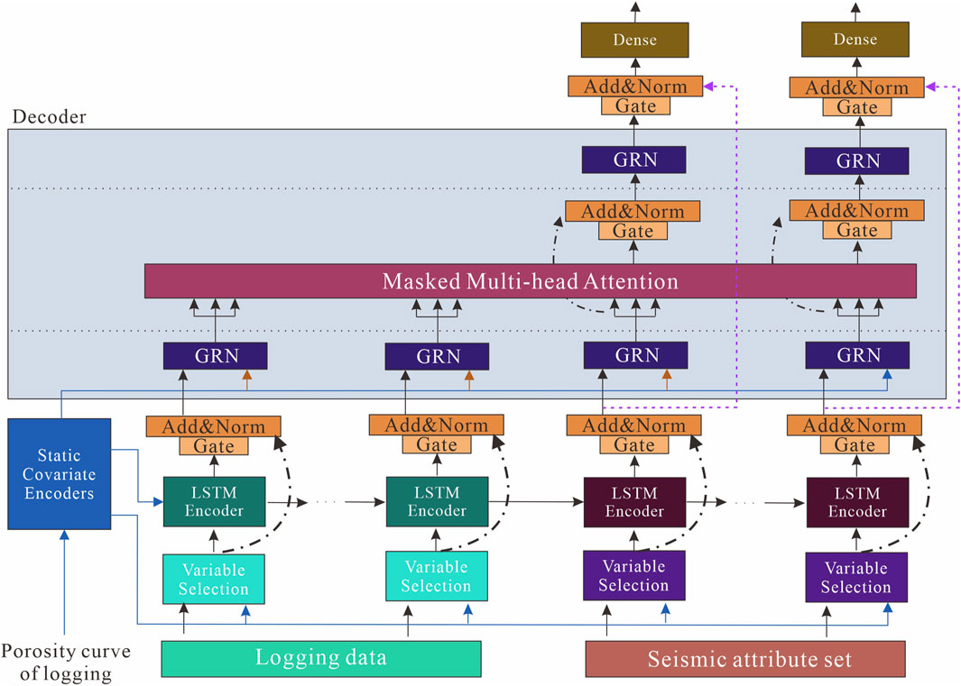
FIGURE 1. Transformer Prediction Network Architecture. GRN and LSTM are gated residual network and Long Short-Term Memory network, respectively.

2.1 Multi-headed attention mechanism

Seismic data is a type of sequence data, and the attention mechanism is inspired by the selective attention mechanism of human vision, which focuses on critical information while ignoring secondary information. It allows sifting through complex data to find helpful information for the present. The core idea of the attention mechanism is to selectively focus on input information by assigning weights that filter out less important information from a large amount of data. The multi-headed attention mechanism is the key component of the Transformer architecture, entirely based on the attention mechanism. It uses multiple copies of the single-headed attention mechanism to extract different information, and the outputs of these heads are concatenated and passed through a fully connected layer to produce the final output.

The multi-headed attention mechanism is defined as follows (Vaswani et al., 2017):

$\left[Q,K,V\right]=P_{QKV}\left(z_t\right)(1)$

$Attention\left(Q,K,V\right)=\mathrm{s}\mathrm{o}\mathrm{f}\mathrm{t}\mathrm{m}\mathrm{a}\mathrm{x}\left(\frac{Q{K}^T}{\sqrt{D}}\right)V(2)$

Where $Q$ denotes the information query set, $K$ is the corresponding similarity set, and $V$ denotes the value set. The matrices of $Q$, $K$ and $V$ are projected by the inputs in the attention module using the fully connected layer shown in Eq 1. The scaling factor $1/\sqrt{D}$ is applied to the parametric gradient, the softmax function such that the sum of $Q{K}^T/\sqrt{D}$ is equal to 1. The attention weight is denoted as $\mathrm{W}=\mathrm{s}\mathrm{o}\mathrm{f}\mathrm{t}\mathrm{m}\mathrm{a}\mathrm{x}\left(Q{K}^T/\sqrt{D}\right)$, where $W$ is based on the pairwise correlation between the query set $Q$ and the key set $K$, $D$ denotes the dimension of the sequence. In addition, the attention weights allow us to extract relevant features using the value set V. For more details on the Transformer architecture, refer to Vaswani et al. (2017).

When using the LSTM network alone to input a long sequence for prediction, the gradient update may decay quickly, hindering the update of sequence data to some extent and making it challenging to represent the feature vector effectively. Additionally, subsequent input data also overwrites the previous input, resulting in the loss of details. However, by using the multi-head attention module and performing a linear transformation to generate $Q$, $K$, and $V$ matrices, after expanding the original low-dimensional information to a higher dimension, taking into account the differences between seismic data and natural language, and at the same time having the interaction capability of global information for the input of long sequence multiple seismic attribute data. It not only enhances the influence of strong signals of seismic attribute data but also focuses on weak signal anomalies, avoiding the problem of losing important feature information and reducing the interference of unnecessary information in the sequence. The joint LSTM can effectively learn the rich features and laws in the input data to obtain the porosity data in dense reservoirs. Therefore, the attention mechanism is auxiliary in extracting complex data features.

2.2 Variable selection and gating network

According to the Temporal Fusion Transformer architecture (Lim B et al., 2021), some modules were modified accordingly for the large seismic data volume. We added a gating and variable selection network to the Transformer for seismic data.

In geological studies, lithology typically varies with depth Logging data provides information about the formation rocks, while seismic attributes reflect different features of the formation. The corresponding values for porosity prediction should be a weighted sum of adjacent characteristic responses that have a certain correlation with each other. Therefore, when we establish the relationship between porosity and external input of various seismic attributes, we should consider the local correlation, the trend of change with depth, and the relationship of adjacent strata. However, since the relationships between external seismic attribute inputs are unknown and uninterpretable for porosity prediction, it is difficult to determine which variables are correlated and the degree of nonlinear processing required. In summary, we need a module for the nonlinear processing of the inputs in this network, so we added a gated residual network (GRN) as a building block for our network. The GRN would accept a primary input $\mathbf{a}$ and context vector $\mathbf{c}$, giving it the functionality to obtain more accurate and comprehensive features.

$GR{N}_{\omega }\left(\mathbf{a},\mathbf{c}\right)=LayerNorm\left(\mathbf{a}+GL{U}_{\omega }\left({\mathbf{\eta }}_{\mathbf{1}}\right)\right)(3)$

${\mathbf{\eta }}_{\mathbf{1}}={\mathbf{W}}_{1,\omega }{\mathbf{\eta }}_{\mathbf{2}}+{\mathbf{b}}_{1,\omega }(4)$

${\mathbf{\eta }}_{\mathbf{2}}=ELU\left({\mathbf{W}}_{2,\omega }\mathbf{a}+{\mathbf{W}}_{3,\omega }\mathbf{c}+{\mathbf{b}}_{2,\omega }\right)(5)$

Where ELU denotes the unit activation function (Clevert, Unterthiner, & Hochreiter, 2016), ${\mathbf{\eta }}_{\mathbf{1}}\in {\mathbb{R}}^{d_{model}}$, ${\mathbf{\eta }}_{\mathbf{2}}\in {\mathbb{R}}^{d_{model}}$ are intermediate layers, $LayerNorm$ is a standard layer normalization by Lei Ba, Kiros and Hinton (2016), $\omega$ is the metric indicating weight sharing, ${\mathbf{b}}_{\left(·\right)}\in {\mathbb{R}}^{d_{model}}$ are the weights and biases. The ELU activation function will then function as a recognition function when ${\mathbf{W}}_{2,\omega }\mathbf{a}+{\mathbf{W}}_{3,\omega }\mathbf{c}+{\mathbf{b}}_{2,\omega }$ is greater than zero, and ELU activation will produce a constant output when ${\mathbf{W}}_{2,\omega }\mathbf{a}+{\mathbf{W}}_{3,\omega }\mathbf{c}+{\mathbf{b}}_{2,\omega }$ is less than zero. We use a component gating layer based on Gated Linear Units (GLUs) (Dauphin et al., 2017) to provide flexibility to suppress certain repetitions of unwanted parts of a particular seismic attribute dataset.

The variable selection also allows TP to remove any unnecessary noisy inputs that may negatively affect the prediction. However, identifying null or invalid values of the seismic attribute data manually in a large work area can be time-consuming and laborious. Hence, we introduced a variable selection module (Gal & Ghahramani, 2016) to automate this process. A linear transformation of the variables is also applied to convert each post-input variable into a d-dimensional vector, which matches the dimensions in the subsequent layers and is mainly used to achieve jump connections. The weights vary for different data (determined by the correlation of each attribute with the porosity). The variable selection network on the seismic data input is presented below, as shown in Figure 2. Note that the variable selection network is the same for the other data set inputs.

FIGURE 2

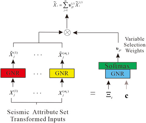
FIGURE 2. Variable selection network.

We denote $X_i^{\left(j\right)}\in {\mathbb{R}}^{d_{model}}$ as the $j_{th}$ variable input value in a time-domain earthquake sequence, where ${\mathrm{\Xi }}_i={\left[X_i^{{\left(1\right)}^T},\dots ,X_i^{{\left(m\right)}^T}\right]}^T$ is the flattened vector of which all have been entered. The weights for variable selection are then generated by feeding both ${\mathrm{\Xi }}_i$ and additional context vectors $\mathbf{c}$ into GRN and then into the Softmax layer:

${\mathbf{\upsilon }}_{\chi t}=\mathrm{S}\mathrm{o}\mathrm{f}\mathrm{t}\mathrm{m}\mathrm{a}\mathrm{x}\left(GR{N}_{\upsilon \chi }\left({\mathrm{\Xi }}_t,\mathbf{c}\right)\right)(6)$

Where ${\mathbf{\upsilon }}_{\chi t}\in {\mathbb{R}}^{m_{\chi }}$ is the vector of variable selection weights and $\mathbf{c}$ is obtained from the static covariate encoder (Section 2.3).

An additional non-linear processing layer is applied during the input process by passing each sequence element through its own GNR.

${\stackrel{\sim }{X}}_i^{\left(j\right)}=GR{N}_{\stackrel{\sim }{X}\left(j\right)}\left(X_i^{\left(j\right)}\right)(7)$

where ${\stackrel{\sim }{X}}_i^{\left(j\right)}$ is the feature vector after processing the seismic attribute $j$. We note that each sequence has its own $GR{N}_{\stackrel{\sim }{X}\left(j\right)}$, and the weights are shared globally. The processed features are then weighted and combined according to their variable selection weights as follows:

${\stackrel{\sim }{X}}_i={\displaystyle \sum _{j=1}^m}{\mathbf{\upsilon }}_{\chi t}^{\left(j\right)}{\stackrel{\sim }{X}}_i^{\left(j\right)}(8)$

Where ${\mathbf{\upsilon }}_{\chi t}^{\left(j\right)}$ is the $j_{th}$ element of vector ${\mathbf{\upsilon }}_{\chi t}$.

In summary, the correlation between seismic attribute data and porosity is unknown, and adding the GRN module provides the advantage of complementing the seismic attribute preference. Additionally, because the input of various seismic attribute data may contain many invalid values, the variable selection network is used to further optimize the input data and prevent significant errors in the prediction results.

2.3 Static covariant encoder

Due to the variation of rock properties with depth and the correlation between seismic response adjacencies, it is crucial to consider not only the local correlation between seismic attribute data but also the trend of seismic data with depth and adjacency information when establishing the mapping relationship between different attribute data and porosity. The TP model can integrate information from the logging porosity data. A separate GNR encoder is then used to generate a context vector. The context vectors are connected to different locations in the network architecture where static variables play an essential role. These include the selection of data for additional seismic attributes, the underlying processing of features, the use of logging curves to guide the identification of the context vector, and the enrichment of features for data adjacency.

2.4 Decoder

We have considered the use of the LSTM encoder-decoder as a building block for our prediction architecture, following the success of this approach in typical sequential coding problems (Wen et al., 2017; Fan et al., 2019; Wang et al., 2022). Due to the specificity of seismic data, the critical points in the data we apply are usually determined based on the surrounding values. Therefore, we propose to use a sequence-to-sequence layer to process the data naturally. Send $X_{i-k:i}$ to the encoder and $X_{i+k:i+{\tau }_{\max }}$ to the decoder. A set of uniform features is generated as input to the decoder itself, using $\varphi \left(i,n\right)\in \left\{\varphi \left(i,-k\right),\dots ,\varphi \left(i,{\tau }_{\max }\right)\right\}$, and $n$ is a position index. In addition, to allow static metadata to affect local processing, we use a context vector from a static covariate encoder to initialize the cell state and hidden state of the first LSTM in the layer, respectively. We also employ a gated jump connection on this layer at:

$\stackrel{\sim }{\varphi }\left(i,n\right)=LayerNorm\left(X_{i+n}+GL{U}_{\stackrel{\sim }{\varphi }}\left(\varphi \left(i,n\right)\right)\right)(9)$

Where $n\in \left[-k,{\tau }_{\max }\right]$ is a location index, $i$ denotes the $i_{th}$ sequence data.

Since static covariates often have an enormous impact on features, we introduce a layer simultaneously to augment the corresponding features with static metadata. For a given location index $n$, the form of:

$\theta \left(i,n\right)=GR{N}_{\theta }\left(\stackrel{\sim }{\varphi }\left(i,n\right),\mathbf{c}\right)(10)$

Where the whole layer shares the weights of $GR{N}_{\theta }$, and $\mathbf{c}$ is the context vector from the static covariate encoder. Finally, the attention layer, the decoder mask (Vaswani et al., 2017; Li et al., 2019b), is applied to the multi-head attention mask layer to ensure that each dimension notices its previous features.

3 A case study

3.1 Data preparation

Considering the completeness and universality, many seismic attributes need to be extracted, resulting in redundant information. Seismic attribute optimization is to preferably select the attributes with better correlation with the target reservoir parameters from a large number of attributes to eliminate the redundant information and thus improve the prediction accuracy. The preferred effect of seismic attributes is often reflected in oil and gas prediction results. In this study, the analysis of the rendezvous plots was first conducted using the Pearson correlation coefficient (PCC) as the criterion. The PCC reflects the degree of similarity of each unit change between two variables, and the closer the result is to 1 indicates the more significant correlation between the variables, which is calculated by the following equation:

$PCC=\frac{Cov\left(y,\widehat{y}\right)}{{\sigma }_y{\sigma }_{\widehat{y}}}(11)$

Where $Cov\left(y,\widehat{y}\right)$ denotes the covariance of the two variables $y$ and $\widehat{y}$, used to describe the linear relationship between the two variables, and $\sigma$ is the standard deviation.

This study analyzed porosity separately with multiple attributes, and we used the attribute preference method to perform preliminary screening of each seismic attribute. The multiple seismic attributes shown in Table 1 include post-stack seismic attributes and various derived post-stack attributes in order to avoid the multi-solution nature of single-parameter inversion to initially screen out the useless data with enormous influence. Figure 1 shows a representative rendezvous analysis of several attributes, and other rendezvous analyses are also performed in the same way we can select the corresponding seismic attributes. Finally, 12 seismic attribute bodies such as Q Factor, Fluid Factor, PG, P-impedance, and variance are selected as input according to PCC, as shown in Table 2 and Figure 3.

TABLE 1

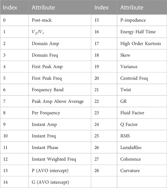
TABLE 1. Optional seismic attributes.

TABLE 2

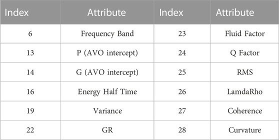
TABLE 2. Input seismic attribute data.

FIGURE 3

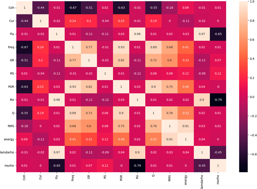
FIGURE 3. Seismic attributes and porosity intersection map.

3.2 Evaluation criteria

This study uses three primary metrics to evaluate the performance of porosity prediction, namely, mean square error (MSE), Pearson correlation coefficient (PCC), and coefficient of determination ($R^2$), to quantitatively evaluate the inversion results.

Mean squared error. MSE is the sum of squares of the corresponding point errors between the predicted and actual data. The smaller the value, the better the fit between predicted and actual data. It is defined as shown in Eq 12.

$MSE=\frac{1}{N}{\sum }_{i=1}^n{\left(y_i-{\stackrel{⌢}{y}}_i\right)}^2(12)$

Where $y_i$ and ${\stackrel{⌢}{y}}_i$ are the predicted and actual values of the series, and $N$ is the number of sampling points.

Pearson Correlation Coefficient. PCC indicates the overall fit between the predicted and actual data. Its range is [-1,1]. The larger the value, the stronger the linear correlation. It is defined in Eq 11.

Coefficient of determination. $R^2$ is used to assess the fit between the variables and considers the mean square error between the predicted and actual data. It ranges from [0,1]. The larger the value, the better the fit between the variables. The following equation gives it:

$R^2=1-\frac{{{\sum }_{i=1}^n\left(y_i-{\stackrel{⌢}{y}}_i\right)}^2}{{{\sum }_{i=1}^n\left(y_i-{\overline{y}}_i\right)}^2}(13)$

Where $\overline{y}$ is the average value of $y_i\left(i=\mathrm{1,2},...,n\right)$.

3.3 Experiment and result analysis

In order to assess the validity of our proposed method, we conducted a method analysis experiment using logging data from two wells, X and Y, in a dense sandstone reservoir in an actual working area. The logging depth of well X was between 2750 m and 2940m, while that of well Y was between 2714m and 2870 m. The logging curves included porosity, density, spontaneous potential, p-wave velocity, natural gamma ray, deep lateral resistivity, compensated neutron, and others. After removing any outliers, we obtained two sets of logging data from wells X and Y for training and test datasets in the Transformer architecture. First, we screened the sensitive parameters of well X using Pearson correlation coefficients. Next, we used the Transformer model built with the logging data of well X to predict the porosity of well Y. To compare our model with other existing models, we also used bi-directional Long Short-Term Memory (BLSTM) and convolutional neural network (CNN) in this experiment.

The correlation between the porosity and other logging parameters was obtained by correlating the petrophysical logging parameters of the two test study wells, as shown in Figure 4.

FIGURE 4

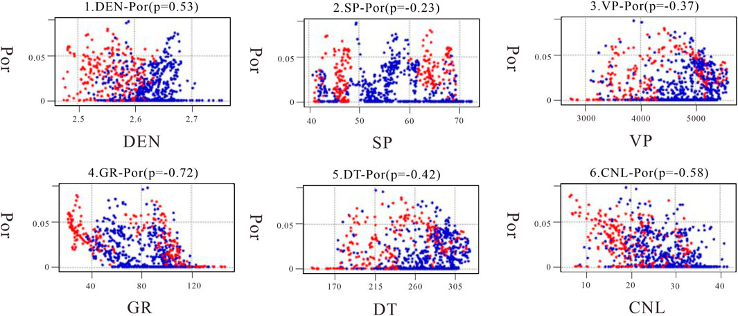
FIGURE 4. Logging parameters and porosity intersection map.

The logging parameters selected for this study are density (DEN), spontaneous potential (SP), p-wave velocity (VP), natural gamma (GR), acoustic log(DT), and compensate neutron log(CNL). From the correlation graph shown in Figure 4, it is evident that CNL, DEN, DT, and GR are highly correlated with porosity (POR), whereas natural potential and longitudinal velocity exhibit weaker correlations. Therefore, we have used the four input datasets with higher correlation for predicting porosity in tight reservoir logs. In this study, we have used Root Mean Square Error (RMSE), Mean Absolute Error (MAE), and Mean Absolute Percentage Error (MAPE) as evaluation metrics to assess the performance of the model. These metrics measure the deviation between the predicted and actual data, with lower values indicating better performance.

We trained the model on the preferred well X data and used it to predict the porosity of well Y. The results of the prediction are presented in Figure 5. Using deep learning techniques and sensitive feature parameters, such as CNL, DEN, DT, and GR, we obtained good results in porosity prediction of wells. Three models, namely, Transformer, BLSTM, and CNN, were used for porosity prediction, and while errors existed, the overall fit to the actual porosity curve was satisfactory. As illustrated in Figure 5, the predicted values of the Transformer model were closer to the actual values than those of the BLSTM and CNN models, especially in the areas of significant variation, where the results were more satisfactory. The prediction errors are summarized in Table 3, and it can be concluded that the Transformer model has more advantages.

FIGURE 5

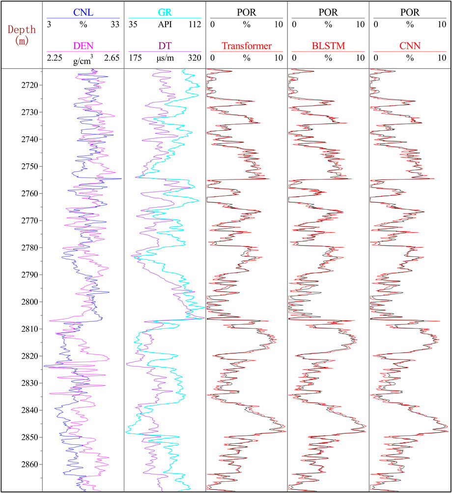
FIGURE 5. Results of porosity prediction across wells with different models (well Y).

TABLE 3

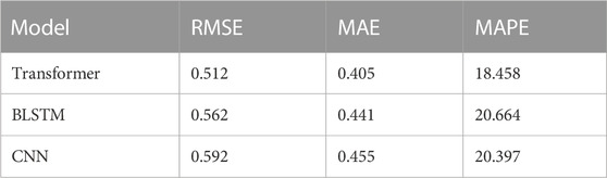
TABLE 3. Porosity prediction error for well Y.

In this study, we applied the model to the actual data of an exploration area in eastern Sichuan for tight sandstone oil and gas exploration. It is difficult to describe the reservoir in this exploration area; the seismic response of the submerged river sand body is not obvious and variable, the reservoir thickness of the river sand body is large, but the porosity is small, the porosity prediction is difficult, and it is a dense gas reservoir. We used the logging data of 5 wells and optimized 12 types of seismic volume attribute data in this work area. We divided our dataset into three parts - a training set for learning, a validation set for hyperparameter tuning, and a test set reserved for performance evaluation. For hyperparameter optimization, we use the random search method. Table 4 shows the entire search range of all hyperparameters as follows and the optimal model parameters.

● State Size–10,20,40,80,160,240

● Dropout rate–0.1, 0.2, 0.3, 0.4, 0.5, 0.7, 0.9

● Minibatch size–64, 128, 256

● Learning rate–0.0001, 0.001, 0.01, 0.1

● Max. gradient norm–0.01, 1.0, 100.0

● Num. heads–1, 4

TABLE 4

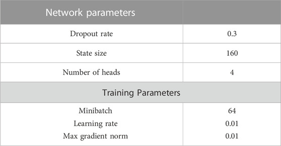
TABLE 4. Optimal network parameters.

During the training process of our dataset, a significant amount of seismic data input is required. However, using the basic architecture of the Transformer model, the entire architecture can be deployed on a single GPU without consuming many computer resources. For instance, when we used NVIDIA Quadro GP100 GPU for the experimental data, our optimal parameter TP model only required less than 2 hours to complete training. Figure 6 presents the comparison of well porosity prediction results, in which the red curve is the actual value, the blue curve is the CNN prediction value, the purple curve is the BLSTM prediction value and the green curve is the TP prediction value. With the CNN and BLSTM data were added to compare network effects in this study. From the comparison in the figure, we can find that the prediction result of TP is more accurate than CNN or BLSTM, and the mean square error (MSE), Pearson correlation coefficient (PCC), and are used as regression evaluation indicators. Table 5 selects four wells (coded by A, B, C, and D), and it can also be proved from Table 5 that our TP can obtain more accurate results.

FIGURE 6

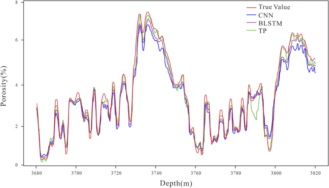
FIGURE 6. Comparison of well porosity prediction results.

TABLE 5

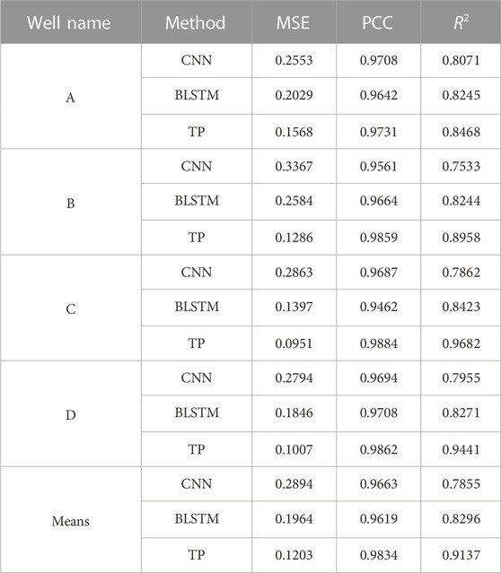
TABLE 5. Comparison of the porosity prediction errors of different models; “Means” indicates the average value of the prediction errors of different methods; “TP” indicates that Transformer Prediction.

Figure 7 shows the porosity result profile predicted by the TP model in this study. Specifically, Figure 7A presents the porosity result profile utilizing standard software for frequency division inversion, whereas Figure 7B represents the porosity inversion of TP training. In the porosity result profile, the red area represents the distribution range of high porosity. The porosity curve of critical well location A in this work area is utilized to verify the prediction results. It is known that the porosity of tight reservoirs inverted by traditional methods is generally small. The important basis is the well-logging porosity, which is significantly affected by the logging data, so the overall resolution is low. Figure 7A also proves that the overall porosity resolution inversion of the tight reservoir is not high, and the lateral continuity is poor. During porosity comparison with logging, the overall porosity in Figure 7A is relatively small due to the complex characteristics of tight reservoirs. However, it can be found from the logging report that the actual porosity range is 0–8%. Hence, the single inversion method still has limitations and does not match the porosity reservoir characteristics of the actual work area. In contrast, Figure 7B illustrates the resulting porosity profile predicted by the TP model. It is observed that the high values are also concentrated near Well A compared to Figure 7A. The overall porosity range also reaches 0–8%, but Figure 7B has a higher resolution. The comparison around 2058 ms shows that the porosity distribution in Figure 7B is more accurate in the lateral direction. Figure 7A shows that the traditional method cannot accurately invert the pore distribution in the right half, far away from the well location, due to the limitation of logging data. Table 6 shows the well and porosity profile prediction and the MSE, PCC, and $R^2$ of logging and input porosity profile, respectively.

FIGURE 7

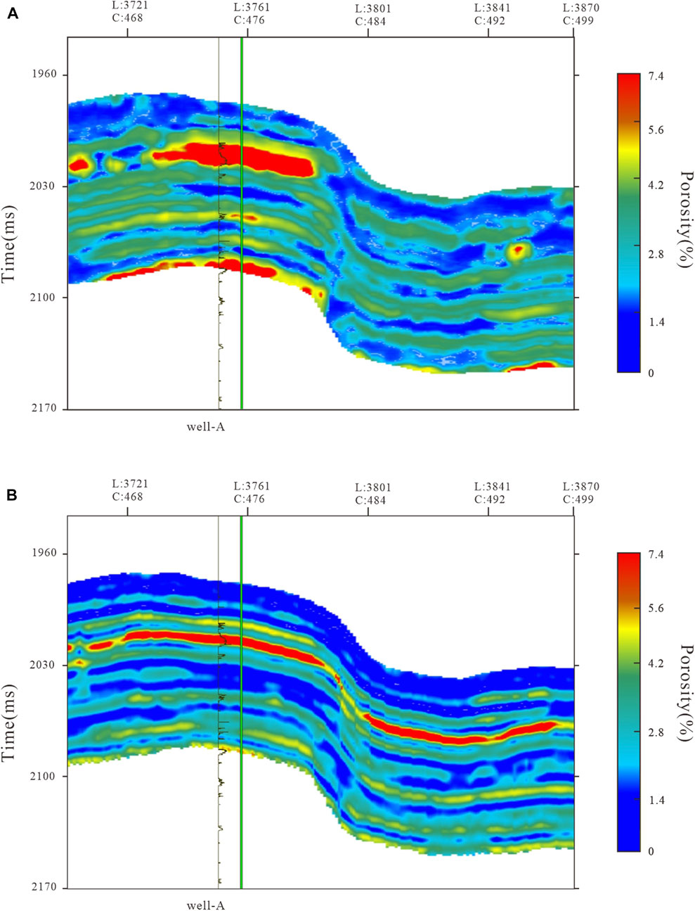
FIGURE 7. Section of porosity results. (A). Frequency division inversion porosity profile; (B). TP predicted porosity profile.

TABLE 6

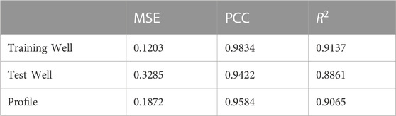
TABLE 6. Prediction of well and porosity profile and MSE, PCC and $R^2$.

4 Discussion

In the previous experiment, the Transformer model’s RMSE, MAE, and MAPE metrics for well X were 8.91%, 8.16%, and 10.68% lower than those of the BLSTM, respectively, and 13.51%, 10.98%, and 9.51% lower than those of the CNN. Although the overall effect was not as good as that of the well porosity prediction, the effect was more evident and reflected the generalization ability of the proposed method. Subsequent experiments comparing TP with several deep learning methods showed that the proposed method had high accuracy and strong continuity in predicting the porosity of dense reservoirs. The MSE, PCC, and $R^2$ of predicted actual data porosity were 0.1203, 0.9834, and 0.9137, respectively. The MSE of predicted porosity was decreased by 0.1691 and 0.0761 when compared with the CNN-based and BLSTM-based methods, respectively, and the PCC was improved by 0.0171 and 0.0215, and $R^2$ was improved by 0.1282 and 0.0841. The profile application also showed that TP accurately predicted porosity in the training work area (MSE = 0.1872, PCC = 0.9584, $R^2$ = 0.9065). In summary, the TP model had certain advantages and effects regarding overall prediction accuracy and accuracy. Additionally, the TP model had an advantage in predicting the porosity of a tight reservoir, which was generally in line with the sedimentary characteristics of tight sandstone reservoirs. The experimental verification and accuracy analysis of the proposed method proved the effectiveness of the deep learning algorithm in predicting the porosity of tight reservoirs. By combining the particularity of tight reservoirs and the advantages of deep learning algorithms, this paper provided a new method for the porosity prediction of tight reservoirs, which significantly improved the accuracy of porosity prediction in tight reservoirs and provided valuable insights for reservoir exploration and exploitation. However, deep learning is a statistical model that needs to be improved in solving complex earthquake prediction problems in different work areas due to entanglement and multi-solution problems. Therefore, more targeted modules must be added to the model, which may lead to parameter redundancy and higher computational overhead costs that need to be weighed between accuracy and efficiency. To further improve the method model, the Transformer-based encoding-decoding model in porosity prediction may require the addition of appropriate constraints, a smoother loss function, or a more intelligent design, which requires more in-depth research.

5 Conclusion

This paper proposes the TP network model, a new attention-based method for predicting porosity in tight reservoirs, which improves prediction accuracy. During training, TP does not directly map seismic data to inversion parameters. Instead, the network utilizes specialized processing components to target large data of various seismic attributes, including (1) The self-attention mechanism, which enables global information interaction between data and captures deeper feature information, (2) Static covariate encoder, which integrates static metadata into the network and adjusts the data by encoding context vectors, (3) Gated network, which optimizes the transfer of data, and (4) Variable selection, which further optimizes data input. TP predicts porosity by learning the characteristics of logs as well as seismic attribute bodies. The proposed TP inversion network with high resolution, accuracy and horizontal continuity is verified in practical data experiments to effectively predict reservoir porosity in dense formations.

Data availability statement

The original contributions presented in the study are included in the article/supplementary material further inquiries can be directed to the corresponding author.

Author contributions

ZS: Software, Methodology, Writing—original draft; JC: Funding acquisition, Writing—review and editing, Supervision; TX: Methodology, Formal analysis; JF and SS: Data curation, Visualization. All authors contributed to the article and approved the submitted version.

Funding

This work was supported by the National Natural Science Foundation of China (Grant Nos 42030812 and 41974160).

Conflict of interest

The authors declare that the research was conducted in the absence of any commercial or financial relationships that could be construed as a potential conflict of interest.

Publisher’s note

All claims expressed in this article are solely those of the authors and do not necessarily represent those of their affiliated organizations, or those of the publisher, the editors and the reviewers. Any product that may be evaluated in this article, or claim that may be made by its manufacturer, is not guaranteed or endorsed by the publisher.

References

Adelinet, M., and Ravalec, M. L. (2015). Effective medium modeling: How to efficiently infer porosity from seismic data? Interpretation 3 (4), SAC1–SAC7. doi:10.1190/int-2015-0065.1

CrossRef Full Text | Google Scholar

Aditya, R., Mikhail, P., Gabriel, G., Scott, G., Chelsea, V., and Alec, R., (2021). Zero-shot text-to-image generation. https://arxiv.org/abs/2102.12092.

Google Scholar

Avseth, P., Mukerji, T., and Mavko, G. (2010). Quantitative seismic interpretation: Applying rock physics tools to reduce interpretation risk. Cambridge, UK: Cambridge University Press.

Google Scholar

Bahdanau, D., Cho, K., and Bengio, Y. (2014). Neural machine translation by jointly learning to align and translate. https://arxiv.org/abs/1409.0473.

Google Scholar

Bosch, M., Carvajal, C., Rodrigues, J., Torres, A., Aldana, M., and Sierra, J. (2009). Petrophysical seismic inversion conditioned to well-log data: Methods and application to a gas reservoir. Geophysics 74 (2), O1–O15. doi:10.1190/1.3043796

CrossRef Full Text | Google Scholar

Chen, M., and Radford, A. (2020). “Generative pretraining from pixels,” in Proceedings of the ICML, Baltimore, ML, USA, June 2020.

Google Scholar

Clevert, D. A., Unterthiner, T., and Hochreiter, S. (2016). Fast and accurate deep network learning by exponential linear units (ELUs). https://arxiv.org/abs/1511.07289.

Google Scholar

Cornia, M., Stefanini, M., Baraldi, L., and Cucchiara, R. (2020). “Meshedmemory transformer for image captioning,” in Proceedings of the 2020 IEEE/CVF Conference on Computer Vision and Pattern Recognition, CVPR 2020, Seattle, WA, USA, June 2020, 10575–10584.

CrossRef Full Text | Google Scholar

Dauphin, Y., Fan, A., and Auli, M. (2017). “Language modeling with gated convolutional networks,” in Proceedings of the International conference on machine learning, Baltimore, ML, USA, December 2017 (PMLR), 933–941.

Google Scholar

de Figueiredo, L. P., Grana, D., Bordignon, F. L., Santos, M., Roisenberg, M., and Rodrigues, B. B. (2018). Joint Bayesian inversion based on rock-physics prior modeling for the estimation of spatially correlated reservoir properties. Geophysics 83 (5), M49–M61. doi:10.1190/geo2017-0463.1

CrossRef Full Text | Google Scholar

Ding, Ming, Yang, Zhuoyi, and Hong, Wenyi (2021). Cogview: mastering text-to-image generation via transformers. https://arxiv.org/abs/2105.13290.

Google Scholar

Dosovitskiy, Alexey, and Beyer, (2020). An image is worth 16x16 words: Transformers for image recognition at scale. https://arxiv.org/abs/2010.11929.

Google Scholar

Fan, C., Zhang, Y., and Pan, Y. (2019). “Multi-horizon time series forecasting with temporal attention learning,” in Proceedings of the 25th ACM SIGKDD International conference on knowledge discovery and data mining, Long Beach, CA, USA, July 2019, 2527–2535.

CrossRef Full Text | Google Scholar

Feng, R. (2020). Estimation of reservoir porosity based on seismic inversion results using deep learning methods. J. Nat. Gas Sci. Eng. 77, 103270. doi:10.1016/j.jngse.2020.103270

CrossRef Full Text | Google Scholar

Gal, Y., and Ghahramani, Z. (2016). A theoretically grounded application of dropout in recurrent neural networks. Adv. neural Inf. Process. Syst. 29.

Google Scholar

Han, Chi, Wang, Mingxuan, Ji, Heng, and Li, Lei (2021). Learning shared semantic space for speech-to-text translation. https://arxiv.org/abs/2105.03095.

CrossRef Full Text | Google Scholar

Hocheriter, S., Schmidhuber, J., and Cummins, F. (1997). Long short-term memory. Neural comput. 9 (8), 1735–1780. doi:10.1162/neco.1997.9.8.1735

PubMed Abstract | CrossRef Full Text | Google Scholar

Hu, S., Zhu, R., and Wu, S. (2018). Profitable exploration and development of continental tight oil in China. Petroleum Explor. Dev. 45 (4), 737–748. doi:10.11698/PED.2018.04.20

CrossRef Full Text | Google Scholar

Johansen, T. A., Jensen, E. H., Mavko, G., and Dvorkin, J. (2013). Inverse rock physics modeling for reservoir quality prediction. Geophysics 78 (2), M1–M18. doi:10.1190/geo2012-0215.1

CrossRef Full Text | Google Scholar

Leite, E. P., and Vidal, Alexandre C. (2011). 3D porosity prediction from seismic inversion and neural networks. Comput. Geosciences37 8, 1174–1180. doi:10.1016/j.cageo.2010.08.001

CrossRef Full Text | Google Scholar

Lepikhin, D., Lee, H. J., and Xu, Y. (2021). “GShard: Scaling giant models with conditional computation and automatic sharding,” in Proceedings of the International Conference on Learning Representations, Vienna, Austria, May 2021.

Google Scholar

Li, S. (2019b). Enhancing the locality and breaking the memory bottleneck of transformer on time series forecasting. https://arxiv.org/abs/1907.00235.

Google Scholar

Li, S., Liu, B., Ren, Y., Chen, Y., Yang, S., Wang, Y., et al. (2019a). Deep-learning inversion of seismic data. IEEE Trans. Geoscience Remote Sens. 58 (3), 2135–2149. doi:10.1109/tgrs.2019.2953473

CrossRef Full Text | Google Scholar

Lim, B., Arık, S. Ö., Loeff, N., and Pfister, T. (2021). Temporal Fusion Transformers for interpretable multi-horizon time series forecasting. Int. J. Forecast. 37 (4), 1748–1764. doi:10.1016/j.ijforecast.2021.03.012

CrossRef Full Text | Google Scholar

Liu, Ze, Lin, Y., and Cao, Y. (2021). Swin transformer: Hierarchical vision transformer using shifted windows. https://arxiv.org/abs/2103.14030.

CrossRef Full Text | Google Scholar

Pang, M., Ba, J., Carcione, J. M., Zhang, L., Ma, R., and Wei, Y. (2021). Seismic identification of tight-oil reservoirs by using 3D rock-physics templates. J. Petroleum Sci. Eng. 201, 108476. doi:10.1016/j.petrol.2021.108476

CrossRef Full Text | Google Scholar

Song, W., Feng, X., and Wu, G. (2021). Convolutional neural network, res-unet++, based dispersion curve picking from noise cross-correlations. J. Geophys. Res. Solid Earth 126 (11), e2021JB022027. doi:10.1029/2021JB022027

CrossRef Full Text | Google Scholar

Us Energy Information Administration(Eia), (2013). Outlook For Shale Gas And Tight Oil Development In The Us. Washington, DC, USA: US Energy Information Administration

Google Scholar

Vaswani, A., Shazeer, N., and Parmar, N. (2017). Attention is all you need. Adv. neural Inf. Process. Syst. 30.

Google Scholar

Wang, J., Cao, J., and You, J. (2020b). Log reconstruction based on gated recurrent unit recurrent neural network. Seg. Glob. Meet. Abstr. Society of Exploration Geophysicists, 91–94. doi:10.1190/iwmg2019_22.1

CrossRef Full Text | Google Scholar

Wang, J., Cao, J., and Yuan, S. (2022a). Deep learning reservoir porosity prediction method based on a spatiotemporal convolution bi-directional long short-term memory neural network model. Geomechanics Energy Environ. 32.doi:100282

CrossRef Full Text | Google Scholar

Wang, P., Chen, X., Li, J., and Wang, B. (2020a). Accurate porosity prediction for tight sandstone reservoir: A case study from North China. Geophysics 85 (2), B35–B47. doi:10.1190/geo2018-0852.1

CrossRef Full Text | Google Scholar

Wang, Y., Niu, L., Zhao, L., Wang, B., He, Z., Zhang, H., et al. (2022b). Gaussian mixture model deep neural network and its application in porosity prediction of deep carbonate reservoir. Geophysics 87 (2), M59–M72. doi:10.1190/geo2020-0740.1

CrossRef Full Text | Google Scholar

Wen, R. (2017). A multi-horizon quantile recurrent forecaster. https://arxiv.org/abs/1711.11053.

Google Scholar

Zheng, M., Gao, P., and Wang, X. (2020). End-to-end object detection with adaptive clustering transformer. https://arxiv.org/abs/2011.09315.

Google Scholar

Zhu, X., Su, W., and Lu, L. (2020). Deformable DETR: deformable transformers for end-to-end object detection. https://arxiv.org/abs/2010.04159.

Google Scholar

Zou, C., Tao, S., and Hou, L. (2014). Unconventional petroleum geology. Beijing, China: Geological Publishing House.

Google Scholar

Zu, S., Ke, C., Hou, C., Cao, J., and Zhang, H. (2022). End-to-End deblending of simultaneous source data using transformer. IEEE Geoscience Remote Sens. Lett. 19, 1–5. doi:10.1109/lgrs.2022.3174106

CrossRef Full Text | Google Scholar