Numerical simulation inversion of creep laws of composite salt layers based on reaming while drilling

1 Research background

Salt-gypsum beds refer to rock beds mainly composed of salts or gypsum. In the petroleum drilling industry, formations predominantly consisting of sodium chloride or other water-soluble inorganic salts, such as potassium chloride, magnesium chloride, calcium chloride, and gypsum or mirabilite, are referred to as salt-gypsum formations. Statistics show that salt rocks in sedimentary basins are the best caprocks, below which 80%–90% of the global oil and gas resources are stored. Therefore, salt-gypsum beds have attracted high attention in both the global petroleum industry and the development of China’s oil and gas resources (Li et al., 2019). Composite salt rocks in Tarim present a high flow capability under high temperature and high pressure. If the drilling fluid fails to maintain the proper performance during drilling, downhole accidents, such as hole shrinkage, sticking, and wellbore collapse, may be caused in a short time. The pressure-bearing capacity of inter-salt formations is low and tensile fractures that can trigger severe lost circulation are highly likely to occur, as the drilling fluid column pressure exceeds the breakdown pressure of inter-salt formations. Creep-induced hole shrinkage and blocking/sticking accidents in salt rocks are relatively severe. Statistics of field accidents occurring in the one typical group report more than 1,000 blocking, more than 100 lost circulations, and nearly 50 well kick events, and the accidents in gypsum-salt beds account for 49% of drilling accidents of the typical group—the gypsum-salt interval, a composite of salt rock, mudstone, and sandstone, is highly troublesome. The most frequent accident is blocking/sticking and 46% of formations found with blocking/sticking accidents are salt rock-bearing.

In view of the creep mechanical properties of salt rocks, scholars of different countries have carried out laboratory experimental studies and predicted the stability of the wellbore in salt beds and the salt cavern gas storage in a theoretical or numerical simulation approach. Farmer and Gilbert, (1984) performed tri-axial experiments on salt rock samples, which showed that salt rock samples present different characteristics, in cases of varied confining pressure. Huang and Deng, (2000) studied the variation law of rheological coefficients of mudstone and salt rocks with the stress, temperature, and water content through a large number of laboratory experiments and theoretical analysis identified the correlations among these parameters, and thus provided critical basic data for understanding the deformation and shrinkage of wellbores in movable formations and calculating the casing external load. Liang and Zhao, (2004) used anhydrous mirabilite salt rocks as salt rock samples to perform uniaxial compression tests and it was shown that the failure mode of anhydrous mirabilite salt rocks is mainly ductile failure during uniaxial compression, with the deformation behavior considerably different from those of conventional rock samples. Jiang et al. (2006) experimentally reported the short-term strength and deformation characteristics of salt rock samples of the Jintan salt mine, Jiangsu Province, China. These samples were characterized by the high transverse deformation capability and high Poisson’s ratio, and correspondingly relatively low elastic modulus and uniaxial compressive strength. Moosavi et al. (2009) carried out laboratory indentation creep tests on salt rocks under different temperatures and stresses and observed creep behaviors under different temperature and stress conditions, which can also be divided into three stages. Their research validated the practicability of the indentation creep test. Li et al. (2009) established a new Cosserat-like constitutive model for bedded salt rocks and made discussion on the stability of salt cavern and natural gas storage. Zeng et al. (2012) developed a finite element method-based three-dimensional model of hole shrinkage in a composite salt layer of interbedding salt rocks and sand-mudstone under the three-dimensional in situ stress condition and quantified the variation of hole shrinkage in the salt layer with the mud density. Based on the constitutive model, Orozco et al. (2018) evaluated the uncertainty and limitation of estimating creep borehole closure during salt rock drilling and delivered the parameter analysis to clarify the influences of the uppermost factors affecting salt creep on borehole closure. This research provided general suggestions for well designers to deal with creep plugging in the case of uncertain salt composition during well planning and drilling operations, so as to prevent harmful drilling events and high economic loss. In terms of the creep of interbedding soft mudstone and salt-gypsum rocks, Lin et al. (2018) established a three-dimensional composite salt layer model of the soft mudstone sandwiched by salt rocks and developed the drilling fluid density plot. Orlic et al. (2019) carried out the geomechanical numerical simulation to estimate the borehole closure time and the results showed that the creep of salt rocks is mainly dependent on the salinity, stress difference, and formation temperature.

Lin et al. (2005) studied the methods for identifying constitutive models of underground salt rocks, established the objective function for the identification of salt rock constitutive models, and developed a displacement back analysis method to determine the creep characteristic parameters of salt rocks, based on borehole caliper measurements. The proposed method can well predict the creep law of downhole salt rocks and hence quantify the hole shrinkage and proper drilling fluid density. Based on the theoretical model analysis, Chen et al. (2014) determined the main influential factors of creep of salt-gypsum rocks and the direct drivers of creep shrinkage, and proposed the inversion method of borehole shrinkage rates and sticking time prediction. Wang et al. (2022) made a lab-scale testing to investigate macro-meso dynamic fracture behaviors of Xinjiang marble. In this research, a numerical simulation method based on reaming while drilling was developed to invert the creep behaviors of composite salt layers. Furthermore, with the actual measurements before and after reaming, the field data were used to validate the inversion results via the theoretical analysis of the salt rock creep pattern and the hole shrinkage numerical simulation at the wellbore scale.

2 The reaming while drilling technology and tools

In terms of the control strategy of creep shrinkage of boreholes in composite salt layers, the application of reaming mainly aims at offering space for the creep of salt layers.

Following the creep mechanism, the wellbore deforms and shrinks after a certain time, which results in accidents like sticking/blocking. The common control method is to properly adjust the drilling fluid density to prevent shrinkage deformation of the borehole wall. However, the drilling difficulty of composite salt layers is attributed to the composite nature of formations—the required drilling fluid densities are different for different lithologies and the requirements on the control practice are more demanding. The strategy behind the reaming-based control technology is to expand the borehole in advance and wait for it to shrink to the original diameter with the elapsed time, and under such circumstances, sticking/blocking can be avoided as long as the time-dependent deformation is well handled, with no need to constantly adjusting the drilling fluid density. The field data show that the reaming effect of hydraulic integrated reaming while drilling is good and the expected reaming effect is achieved. Field applications of the hydraulic integrated reamer while drilling were found with satisfactory reaming while drilling performance.

The reaming technology is an unconventional drilling technology and needs to consider numerous factors, such as operational safety and efficiency, reaming while drilling tools. By whether or not cutting parts are movable, the reamer while drilling can be divided into two types: fixed cutter and movable cutter reamers. Considering the rock mechanical characteristic of fast creep of salt-gypsum layers in the piedmont zone, the Schlumberger (Smith) Rhino XS integrated hydraulic reamer, which is highly reliable with high tensile and torsional resistance and free of limitations by upper casing inner diameters, and presents high hole enlargement rates, was selected.

Tool introduction: Hydraulic reamers are hydraulically-actuated expandable reamers. The Rhino XS integrated hydraulic reamer allows reaming while drilling below the casing shoe. It has expandable cutters that can also be withdrawn. When the tool passes through the wellbore restrictions, the cutter is deactivated and retracted inside the tool body (the deactivation state in Figure 1). Once the tool has passed through restrictions, the tool opens cutters with the help of the pressure difference imposed by the mud and places them against the borehole wall (the activation state in Figure 2). After reaming is completed, the pump is stopped and cutters are retracted back into the tool body—at this state, the tool can again pass through borehole restrictions and thus be tripped out.

FIGURE 1

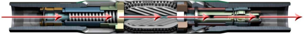
FIGURE 1. Deactivation state of the tool.

FIGURE 2

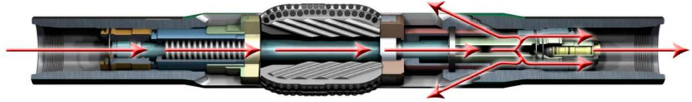
FIGURE 2. Activation state of the tool.

How it works: The hydraulic reamer is driven by hydraulic pressure. The pressure difference acting on the piston inside the tool drives the cutter to move upward along the Z-shaped rail and expand. At the same time, the piston cavity is reduced and the mud was squeezed out from the nozzle, which results in the pressure drop indicative of the opening of cutters. Because of the geometric feature of the Z-shaped cutter groove, the WOB exerted by the hydraulic reamer can keep the opening posture of cutters in the case of forward reaming, and meanwhile, eliminate the vibration of cutters and prolong the service life of PDC composites. The tool structure, specifically the Z-shaped guide rail and the matching cutters, enables adjustable reaming diameters of the tool. A threaded sleeve is installed in the reamer to adjust the opening size of the tool cutter and the opening size of the cutter is constrained within the design range by limiting the moving displacement of the cutter.

Technical features: 1) Reaming can be performed both alone and while drilling. 2) Reaming while drilling can be performed during drilling drillable cement plugs with no need to trip out of hole. 3) It is compatible with the rotary steering system (RSS). 4) The borehole can be enlarged to 125% of the tool size. 5) The PDC cutter is fixed as splines instead of hinges, which enables back reaming and centralizing. 6) The integrated design enhances the torsion resistance and tensile strength of the tool, and the nozzle design on the tool body enhances the hydraulics of the tool, which is beneficial for the clean-up of cuttings.

3 Mechanical model of salt layer creep mechanisms

The composite salt layer is mainly composed of salt rocks, gypsum, gypsum-mudstone, and mudstone-gypsum rock, with thin interbeds of mudstone and muddy siltstone. Salt layers are highly movable under high temperatures and high pressure, which leads to high odds of sticking attributed to creep shrinkage, especially in deep wells. The creep rate of salt layers under high temperature can be high up to causing immediate borehole closure and thus locking of the bit.

Extensive studies have revealed the following creep constitutive relation of gypsum-salt layers and Figure 3 illustrates a typical creep curve. At t=0, the loading starts and the resultant deformation of the specimen is elastic. The creep curve is divided into three stages. The first stage is the transition stage, in which the strain rate decreases with the elapsed time. The second stage is the steady creep stage, in which the strain rate is constant. The third stage is the accelerated creep stage, in which the strain rate increases gradually until the final shear failure of the rock specimen. The creep stages I and II are critical for drilling. The first stage lasts for a very short time and the creep magnitude is small, while the second stage lasts for a rather long time and the creep magnitude of salt rocks can be measured using the corresponding strain. The steady creep rate of salt rocks is highly dependent on the structure and composition of salt rocks and the temperature and pressure to which salt rocks are exposed. To study the rheological properties of specific salt rocks is to determine the relationship between the steady creep rate and temperature and pressure, namely the creep equation.

FIGURE 3

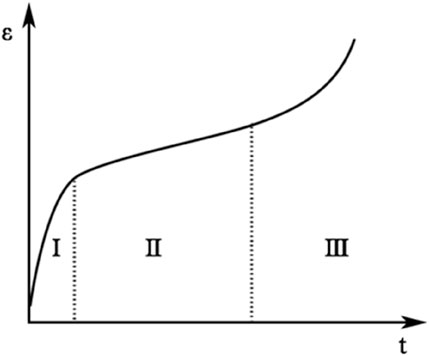
FIGURE 3. A typical creep curve.

The long-term creep behavior of salt rocks is uncertain. Generally, the creep behavior of salt rocks is measured at the laboratory scale. In laboratory deformation experiments, the differential stress is 1 MPa or higher, and the typical strain rate ranges from 10⁻⁹ s⁻¹ to 10⁻⁶ s⁻¹. We developed a long-term creep model for salt rocks, which takes into account the first-order effect of the pressure dissolution creep, grain size, dynamic crystallization, and the composite creep law, and consists of the pressure dissolution and dislocation components. The total strain rate can be divided into transient and steady-state strain rates (mainly manifested as the dislocation and pressure dissolution creep components). The transient part reflects the deformation strain rate of salt rocks from the elastic stage to the steady state stage, while the steady part represents the creep stage of salt rocks with a constant strain rate.

$\dot{\mathit{\epsilon }}={\dot{\mathit{\epsilon }}}_{\mathit{t}\mathit{r}}+{\dot{\mathit{\epsilon }}}_{\mathit{d}\mathit{c}}+{\dot{\mathit{\epsilon }}}_{\mathit{p}\mathit{s}}$

The dislocation creep is expressed as below:

${\dot{\epsilon }}_{dc}=A_{dc}\cdot \exp \left(-\frac{Q_{dc}}{RT}\right){\sigma }^n$

where:

A′—a rheological constant; n—the non-linear coefficient (generally n=4–5 with the maximum value up to 7).

The pressure dissolution creep is expressed below:

${\dot{\epsilon }}_{ps}=A_{ps}\cdot \exp \left(-\frac{Q_{ps}}{RT}\right)\frac{\sigma }{T{D}^m}$

where $A_{ps}$ and $A_{ps}$ are the creep pre-coefficients representing the specific creep mechanisms, the unit is MPa^-ns⁻¹; $Q_{ps}$ and $Q_{dc}$ are the corresponding activation energy parameters; R is the gas constant; T is the absolute temperature; D is the average grain size; $\sigma$ is the second invariant of the deviator stress tensor of the (square root of) effective differential stress; n and m are the exponents of the dislocation creep and grain size, respectively.

Laboratory testing is a direct way to observe the creep characteristics of salt rocks. The flow of salt rocks often occurs at 20°C–200°C. In view of the long-term creep of salt rocks in this temperature range, a large number of laboratory tests have been performed (Spiers et al., 1990; Wawersik and Zimmerer, 1994; Weidinger et al., 1997; Hunsche and Hampel, 1999; Hunsche et al., 2003), of which the results were collected in this research. Figures 4A, B show the relationship between strain rate and deviator stress of salt rocks under steady creep. A part of the salt rock specimens in these tests was collected from the Asse and Gorleben salt domes in Germany, the Avery Island in the Gulf of Mexico, and the southern Oman, and another part was artificial specimens. As illustrated, the steady creep of salt rocks follows two basic creep laws, namely, the power law based on the dislocation creep (the non-Newtonian flow equation) in Figure 4A and the Newtonian flow equation based on the dissolution-precipitation creep in Figure 4B.

FIGURE 4

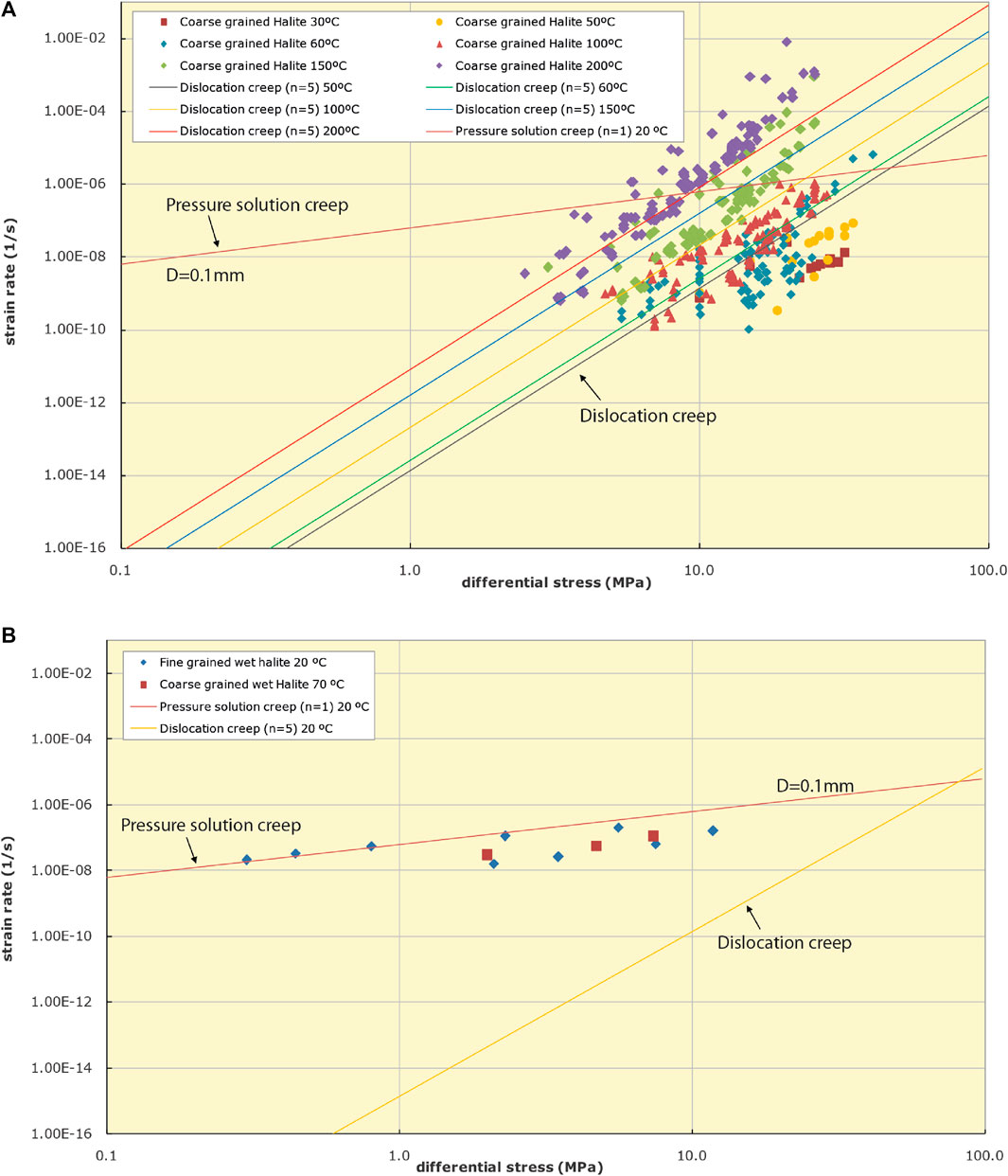
FIGURE 4. (A) Strain rate vs deviator stress controlled by dislocation creep (Li and Urai, 2016). (B). Strain rate vs deviator stress controlled by dissolution-precipitation (or pressure solution) creep (Li and Urai, 2016).

Figure 4A summarized the results of a large number of laboratory tests. Clearly, the relationship between the strain rate and deviator stress of salt rocks is exponential, with an exponent of about 5. This power law indicates that the specimen is controlled by the dislocation creep and reflects the deformation of salt rocks at 20°C–200°C (Weidinger et al., 1997; Hunsche and Hampel, 1999; Hunsche et al., 2003). At each temperature, the variation range of strain rates reaches about 2–3 orders of magnitude in the case of constant deviator stress. Figure 4A demonstrates that the creep of salt rocks is closely related to temperature and the strain rate is higher at a higher temperature. It should be noted that due to the limited experimental time in laboratory tests (the maximum test time lasted about 2–3 years), the high dependence on the crystal grain size, and water content loss in specimens, the dissolution-precipitation creep is rarely reflected in the test results. Therefore, the pattern of the dissolution-precipitation creep is often neglected in the engineering-scale research and application, while the dislocation creep-attributed power law is always regarded as the creep law at the engineering scale (Hunsche and Hampel, 1999; Fossum and Fredrich, 2002). However, the real formation conditions, such as the presence of water in salt rocks and fine crystals, are all critical drivers for the dissolution-precipitation creep deformation, which, in fact, cannot be ignored. Hence, the mechanism of the dissolution-precipitation creep (also referred to as the pressure solution creep) was also incorporated in this research.

In view of the creep law controlled by the dissolution-precipitation (or pressure solution) creep, some laboratory tests have also been carried out (Urai et al., 1986; Spiers et al., 1990; Renard et al., 2004). Salt rock specimens with water content greater than 10 ppm and grain size less than 0.5 mm were used in such tests. Figure 4B summarizes some of the test results—the steady creep strain rate of salt rocks with high water content (also called wet salt) is dependent on three major factors, namely the grain size, water content, and temperature. As shown in Figure 5B, the creep strain rate of fine wet salts (with the grain size of 0.1 mm and water content greater than 10 ppm) at 20°C is above 10⁻⁸ s⁻¹, which is close to that of coarse wet salts (with the particle size of 10 mm and water content greater than 10 ppm) at 70°C. In addition, the water content of salt rock also affects the steady creep.

FIGURE 5

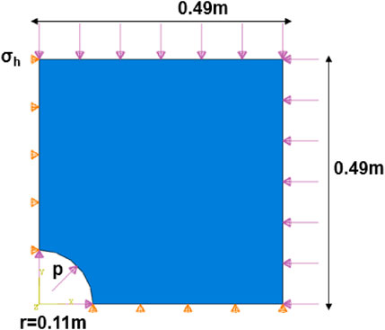
FIGURE 5. Near-wellbore mechanical model.

The creep experiment has been performed at high temperature and high confining pressure on the natural outcrops in the Keshen block of the Tarim oilfield (Liang et al., 2022). According to the experimental data, the deformation of deep salt-gypsum formations is controlled by the dislocation creep mechanism, and the steady-state creep rate of salt rock increases with the increasing temperature and differential stress, of which the expression can be summarized as a stress-independent power law (non-Newtonian body flow) equation.

4 Near-wellbore numerical modeling and field applications of reaming

4.1 Near-wellbore geological and engineering numerical model

The analysis of downhole accidents and complex issues at the regional and well scale can help identify the characteristics of troublesome intervals and is both the premise and foundation of the near-wellbore geological and engineering research. It clearly classifies various accidents, such as blocking, lost circulation, and well kick, and identifies the location and characteristics of troublesome intervals, according to the situation of each well.

The lithologic association of the troublesome interval was identified and the corresponding formation temperature was calculated, according to the geothermal gradient. The geological association provides an important basis for geometric modeling and material modeling of the subsequent geological and engineering models. The lithology distribution of formations is the data basis of multi-layer modeling and a geological engineering model truly reflecting the vertical distribution of formation lithology can be built, in accordance with actual field geological and engineering data.

The wellbore parameters and well trajectory were determined, according to data from drilled wells. They are also an important basis for the geometric modeling of geological and engineering models. Furthermore, the in situ stress profile along the wellbore trajectory was extracted from the three-dimensional stress field based on the lithologic association of the troublesome interval and the wellbore and trajectory data. The stress state is a critical boundary condition of the near-wellbore geological engineering model. The effects of the weight of drilling fluids can be simulated by exerting pressure upon the inner wall of the wellbore. When the geometry, material data, and boundary conditions are all deterministic, the near-wellbore geomechanical model can be developed.

After building the model, it is necessary to define the creep properties, according to the rock materials, and also the creep constitutive relation for the model, according to the laboratory experiments. In this research, the drifting time was set as the simulation time to calculate the drilling fluid density required to prevent sticking and the corresponding creep shrinkage magnitude as well as the shrinkage rate. Among them, the shrinkage rate can be expressed as the ratio of the salt rock shrinkage displacement along the radial direction of the wellbore to the borehole radius (Figure 5).

In addition, the model is a two-dimensional plane strain model. The assumption of plane strain model is:

${\epsilon }_z=0(1)$

${\sigma }_z=\nu \left({\sigma }_x+{\sigma }_y\right)(2)$

among ${\epsilon }_z$ is the strain in the Z direction, ${\sigma }_x{,\sigma }_y{,\sigma }_z$ is the stress in the x, y and z directions, $\nu$ is Poisson’s ratio. Further, the maximum, intermediate and minimum principal stresses ${\sigma }_1,{\sigma }_2$ and ${\sigma }_3$ can be calculated in the plane strain model. The static mechanical equilibrium equation of the model is:

$\frac{\partial {\sigma }_{ij}}{\partial x_j}+{\rho g}_i=0(3)$

Among them, ${\sigma }_{ij}$ is the stress tensor ($i,j=\mathrm{1,2.3}$), ${\rho g}_i$ is a physical item. For the background stress field of the model, the model includes maximum principal stress ${\sigma }_1$, minimum principal stress ${\sigma }_3$ and intermediate principal stress ${\sigma }_2$. The von Mises stress expresses below:

${\sigma }_{\mathrm{V}\mathrm{M}}=\sqrt{\frac{1}{2}\left[{\left({\sigma }_1-{\sigma }_2\right)}^2+{\left({\sigma }_1-{\sigma }_3\right)}^2+{\left({\sigma }_2-{\sigma }_3\right)}^2\right]}(4)$

4.2 Field application of reaming while drilling

(1) The first section is at 4,833–5,525 m. The Pover-V RSS was used during the initial drilling of this section and the corresponding lithology is mainly the white muddy salt rock and brown salty mudstone of the salt rock layer of the typical group. Due to the serious hole shrinkage, during drilling toward 5,525 m, the hole shrinkage was rather considerable—sticking occurred at multiple positions of 4,820–5,124 m and the top drive was forced to shut down many times during back reaming. Subsequently, the BHA consisting of the reamer while drilling + Pover-V RSS was used to separately ream 4,833–5,525 m. The reaming effect was prominent—the average wellbore size was ⌀356.34 mm and the enlargement rate was 6.88%.

(2) The second section is at 5,525–6,543 m. The lithology of this section is mainly brown gypsum-bearing mudstone, gray-white mudstone-gypsum, and brown salty mudstone, with fast creep rates and severe hole shrinkage. The reamer while drilling + Pover-V RSS was used for reaming while drilling. The reaming effect was remarkable, with a resultant average wellbore diameter of 358.62 mm and an enlargement rate of 7.56%, which provides tolerance for creep shrinkage of the salt-gypsum layer (Table 1).

TABLE 1

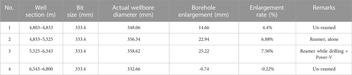
TABLE 1. Detailed data of borehole enlargement.

4.3 Simulation strategy and results

The numerical model was built, based on the field application data. Then, the creep characteristic parameters were continuously adjusted by comparing the numerical simulation results with the actual field data to invert the creep parameters or creep constitutive model. The inversion strategy is summarized below: The horizontal stress difference is limited within a certain range, for example, ΔP = 1 MPa, 5 MPa, 10 MPa, and 15 MPa. Field data include the creep deformation time of 3 days after reaming and the drilling fluid density of 2,300 kg/m³. The first computation is performed, based on the initially assumed creep characteristic parameters; subsequently, the resultant shrinkage deformation was compared with the actual reaming amount in the field; afterward, the second computation is performed, based on the adjusted creep characteristic parameters and the results are compared with the field data. This process is repeated until the shrinkage deformation is consistent with the actual reaming amount (Figure 6).

FIGURE 6

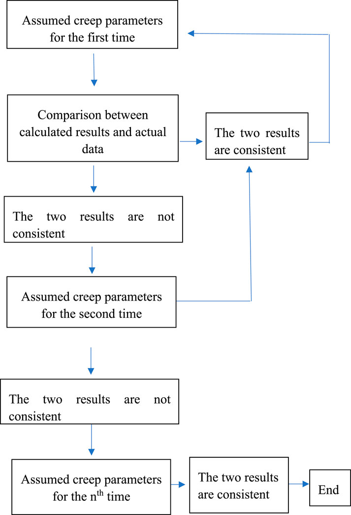
FIGURE 6. Flow chart.

The actual reaming amount is 0.022 m for Layer No. 2 (4,833–5,525 m) and it was modeled according to the actual geological and engineering conditions. When the pressure solution creep mechanism is dominant (n=1) and the horizontal stress difference is 1 MPa, the first-assumed creep parameter A=1.0 × 10⁻¹⁵ produced the maximum hole shrinkage of 0.00899 m; then, the second simulation with the assumed creep parameter A = 1.0 × 10⁻¹³ led to the maximum borehole shrinkage of 0.0724 m; the third simulation with the assumed creep parameter A = 5.0 × 10⁻¹⁴, the maximum borehole shrinkage of 0.0402 m; the fourth simulation with the assumed creep parameter A = 2.6 × 10⁻¹⁴, the calculated maximum borehole shrinkage of 0.022 m, which is consistent with the actual reaming amount. See Table 2 for specific parameters and their values.

TABLE 2

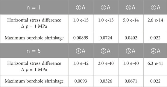
TABLE 2. The pre-coefficient A and the exponent n (Layer No. 2), in the case of n = 1 and n=5.

When the dislocation mechanism is dominant (n=5), the first simulation with the assumed creep parameter A = 1.0 × 10⁻⁴² was found with the calculated maximum borehole shrinkage of 0.0093 m; the second simulation with the assumed creep parameter A = 3.0 × 10⁻⁴⁰, the calculated maximum borehole shrinkage of 0.0326 m; the third simulation with the assumed creep parameter A = 1.0 × 10⁻⁴⁰, the calculated maximum borehole shrinkage of 0.0671 m; finally, the fourth simulation with the assumed creep parameter A = 6.3 × 10⁻⁴¹, the calculated maximum borehole shrinkage of 0.022 m, which is consistent with the actual reaming amount (Table 2).

In cases of varied horizontal stress differences, the differential stresses were set as 1 MPa, 5 MPa, 10 MPa, and 15 MPa, respectively. When the horizontal stress difference is 1 MPa, the pressure solution mechanism is dominant (n = 1), and A =2.6 × 10⁻¹⁴, the near-wellbore stress field after reaming (Figure 7A) shows the near-wellbore Mises stress is about 10 MPa and the differential stress in the far field is 1 MPa. The borehole shrinkage after reaming is shown in Figure 7B—after 3 days, the maximum shrinkage deformation is located at the horizontal endpoint of the wellbore, where the wellbore diameter restores to the original value. When the dislocation mechanism is dominant (n=5) and A = 6.3 × 10⁻⁴¹, the post-reaming near-wellbore stress field distribution (Figure 7C) reveals that the Mises stress around the wellbore is about 6 MPa and the differential stress in the far field is 1 MPa. Moreover, Figure 7D shows the borehole shrinkage after reaming. After 3 days, the maximum shrinkage deformation is evenly distributed around the wellbore—the borehole returns to its original diameter. The case of the horizontal stress difference of 1 MPa indicates that the creep deformation distribution around the well is relatively uniform and the maximum creep deformation occurs around the borehole wall.

FIGURE 7

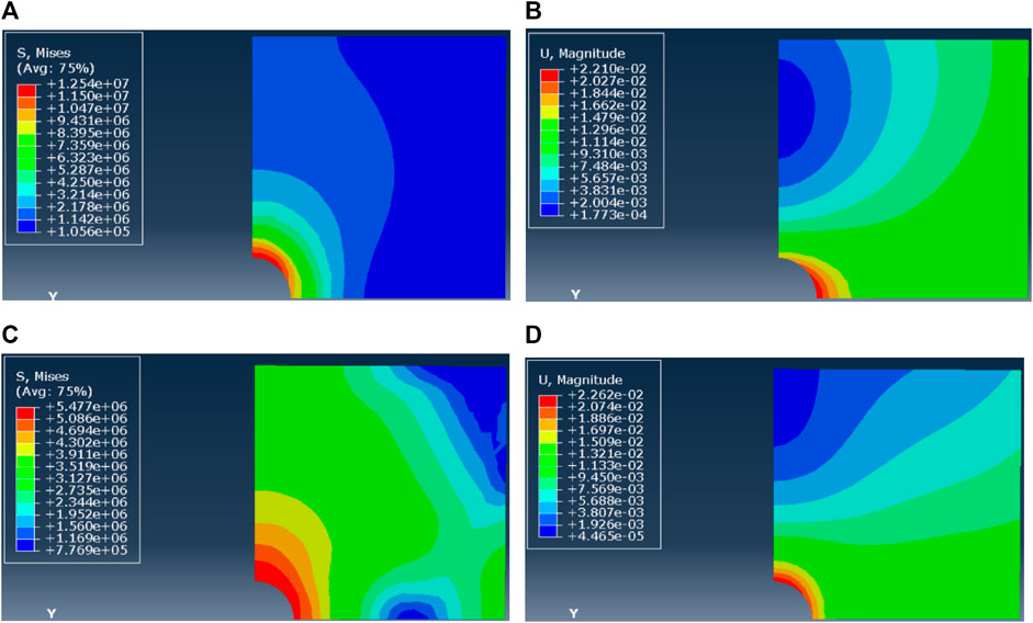
FIGURE 7. (A–D) Mises stress and displacement of borehole shrinkage after reaming (ΔP = 1 MPa, n = 1); Mises stress and displacement of borehole shrinkage after reaming (ΔP = 1 MPa, n = 5)

The simulations in the case of the horizontal stress difference of 5 MPa are presented below. When the pressure solution mechanism is dominant (n = 1), the first simulation with the creep parameter A = 1.0 × 10⁻¹⁵ led to the maximum borehole shrinkage of 0.0172 m; the second simulation with the creep parameter A = 8.0 × 10⁻¹⁴, the maximum borehole shrinkage of 0.096 m; the third simulation with the creep parameter A = 4.0 × 10⁻¹⁴, the maximum borehole shrinkage of 0.052 m; the fourth simulation with the creep parameter A =1.9 × 10⁻¹⁴, the maximum borehole shrinkage of 0.022 m, which is consistent with the actual borehole reaming amount. See Table 3 for specific parameters and their values.

TABLE 3

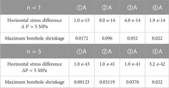
TABLE 3. The pre-coefficient A and the exponent n (Layer No. 3), in the case of n = 1 and n=5.

When the dislocation creep mechanism is dominant (n = 5), the first simulation with the creep parameter A = 1.0 × 10⁻⁴³ gave the maximum borehole shrinkage of 0.00149 m; the second simulation with the creep parameter A = 3.0 × 10⁻⁴¹, the maximum borehole shrinkage of 0.07796 m; the third simulation with the creep parameter A = 1.0 × 10⁻⁴¹, the maximum borehole shrinkage of 0.0376 m; the fourth simulation with the creep parameter A = 5.2 × 10⁻⁴¹, the maximum borehole shrinkage of 0.022 m, which is consistent with the actual borehole reaming result (Table 3).

In the case of the horizontal stress difference of 5 MPa, the dominance of the pressure solution mechanism (n = 1) and A = 2.0 ×10⁻¹⁴, the simulated post-reaming near-wellbore stress field distribution (Figure 8A) shows that the Mises stress around the wellbore is about 10–20 MPa and the differential stress in the far field is 5 MPa. Furthermore, the wellbore shrinkage after reaming is illustrated in Figure 8B—after 3 days, the maximum shrinkage deformation is located at the horizontal endpoint of the wellbore, where the wellbore returns to the original diameter. When the dislocation creep mechanism is dominant (n = 5) and A = 5.2 × 10⁻⁴², the simulated post-reaming stress field distribution around the borehole (Figure 8C) shows that the near-wellbore Mises stress is about 5–10 MPa and the differential stress in the far field is 5 MPa. Furthermore, 3 days after reaming, the maximum shrinkage deformation is evenly distributed around the wellbore and the wellbore returns to the original radius, as is made evident by Figure 8D. In other words, with the horizontal stress difference of 5 MPa, the creep deformation distribution is relatively uniform when the dislocation mechanism is dominant. According to the Mises stress distribution, the stress difference is 1 MPa in the far distance, in the case of the dominance of the pressure solution mechanism; however, it is mostly 3 MPa when the dislocation creep mechanism is dominant.

FIGURE 8

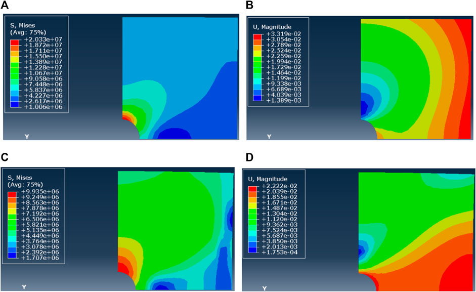
FIGURE 8. (A–D) Mises and displacement of borehole shrinkage after reaming (ΔP = 5 MPa, n = 1). Mises and displacement of borehole shrinkage after reaming (ΔP = 5 MPa, n = 5)

When the horizontal stress difference is 10 MPa and the pressure solution mechanism is dominant, A = 1.7×10⁻¹⁴, n=1. Figure 9A shows the stress field distribution around the borehole wall after reaming. The Mises stress around the borehole is about 5–30 MPa, and the differential stress in the far field is 10 MPa. Figure 9B shows the shrinkage of the borehole wall after reaming. After 3 days, the maximum deformation of shrinkage is located at the end point of the horizontal direction of the borehole and is restored to the original borehole radius. When the dislocation mechanism is dominant, A = 4.0 × 10⁻⁴³, n=5. Figure 9C shows the stress field distribution around the borehole wall after reaming. The Mises stress around the borehole is about 5–17 MPa, and the difference stress in the far field is 10 MPa. Figure 9D shows the borehole wall contraction after reaming. After 3 days, the maximum deformation position of contraction is at the end point of the horizontal direction of the borehole, and it is restored to the original borehole radius position. When the horizontal in situ stress difference is 10 MPa, the creep deformation distribution is no longer uniform when the dislocation mechanism is dominant. From the Mises stress distribution, when the pressure solution mechanism is dominant, the regional stress difference far from the well periphery is 3–4 MPa. While the dislocation mechanism is dominant, the regional stress difference far from the well periphery is mainly 5–6 MPa.

FIGURE 9

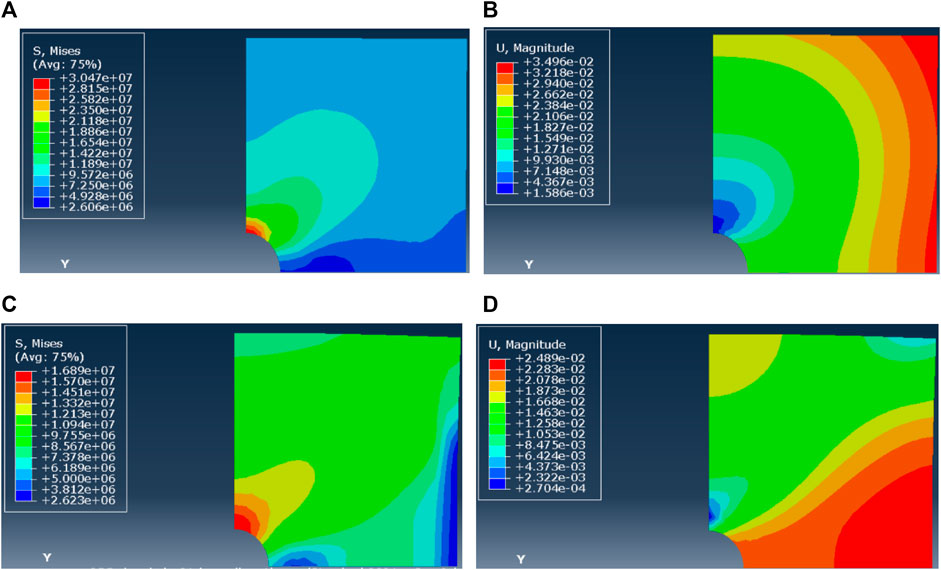
FIGURE 9. (A–D) Mises stress and displacement of borehole shrinkage after reaming (ΔP = 10 MPa, n = 1). Mises stress and displacement of borehole shrinkage after reaming (ΔP = 10 MPa, n = 5)

For the case that the horizontal geostress difference is 15 MPa, when the pressure solution mechanism is dominant (n = 1), the creep parameter is assumed for the first time A=3.0×10^–15, n=1, the calculated maximum borehole diameter reduction is 0.00545 m. The second assumed creep parameter A=2.0×10⁻¹⁴, n=1, the calculated maximum borehole diameter reduction is 0.0525 m. The creep parameter is assumed for the third time A=1.0×10⁻¹⁴, n=1, the calculated maximum borehole diameter reduction is 0.0311 m. The creep parameter is assumed for the fourth time A=7.0×10⁻¹⁵, n=1, the calculated maximum hole diameter reduction is 0.022 m, which is consistent with the actual hole expansion. See Table 4 for specific parameters and values.

TABLE 4

TABLE 4. The pre-coefficient A and the exponent n (Layer No. 2), in the case of n = 1 and n=5.

For the case that the horizontal in situ stress difference is 15 MPa, when the dislocation mechanism is dominant (n = 5), the creep parameter is assumed for the first time A=3.0×10⁻⁴³, n=5, the calculated maximum borehole diameter reduction is 0.0114. The second assumed creep parameter A=3.0×10⁻⁴³, n=5, the calculated maximum borehole diameter reduction is 0.0891 m. The creep parameter is assumed for the third time A=3.0×10⁻⁴³, n=5, the calculated maximum borehole diameter reduction is 0.0316 m. The creep parameter is assumed for the fourth time A=7.0×10⁻⁴³, n=5, the calculated maximum hole diameter reduction is 0.022 m, which is consistent with the actual hole expansion (Table 4).

When the horizontal stress difference is 15 MPa and the pressure solution mechanism is dominant, A= 1.2×10⁻¹⁴, n=1. Figure 10A shows the stress field distribution around the borehole wall after reaming. The Mises stress around the borehole is about 3–40 MPa, and the differential stress in the far field is 15 MPa. Figure 10B shows the shrinkage of the borehole wall after reaming. After 3 days, the maximum deformation of shrinkage is located at the end point of the horizontal direction of the borehole and is restored to the original borehole radius. When the dislocation mechanism is dominant, A = 5.0×10⁻⁴³, n=5. Figure 10C shows the stress field distribution around the borehole wall after reaming. The Mises stress around the borehole is about 4–24 MPa, and the differential stress in the far field is 15 MPa. Figure 10D shows the wellbore shrinkage after reaming. After 3 days, the maximum deformation position of shrinkage is at the end point in the horizontal direction of the wellbore, and it is restored to the original wellbore radius position. From the horizontal difference stress of 15 MPa, when the dislocation mechanism is dominant, the creep deformation distribution is no longer uniform. From the Mises stress distribution, when the pressure solution mechanism is dominant, the stress difference in the area far from the well periphery is 8–12 MPa, while the dislocation mechanism is dominant, the stress difference in the area far from the well periphery is 12–15 MPa.

FIGURE 10

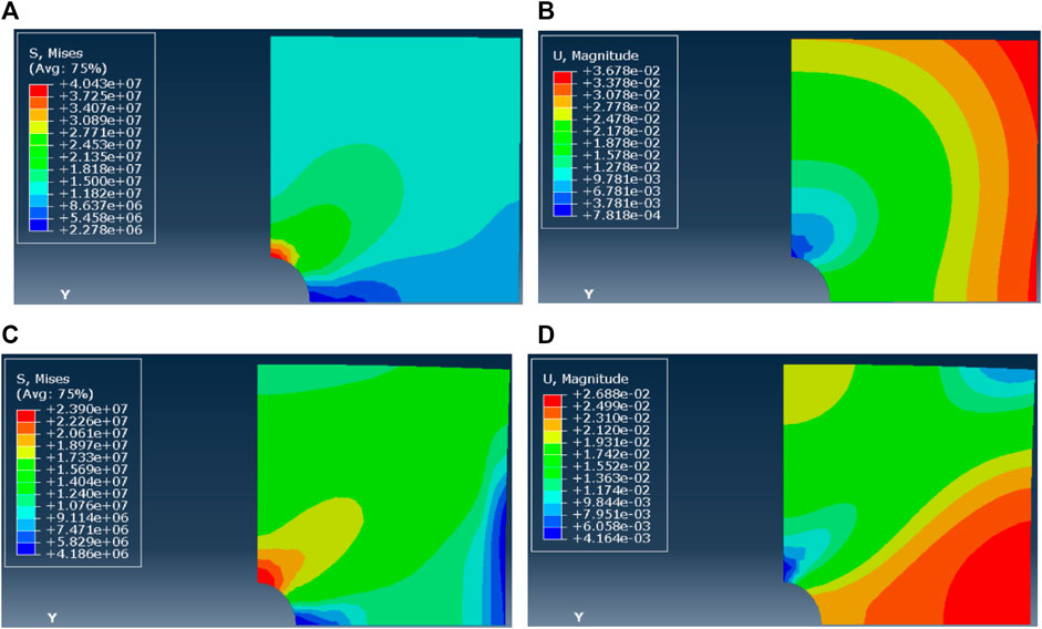
FIGURE 10. (A–D) Mises stress and displacement of borehole shrinkage after reaming (ΔP = 15 MPa, n = 1). Mises stress and displacement of borehole shrinkage after reaming (ΔP = 15 MPa, n = 5)

The inverted creep behavior demonstrates that in the case of the dominance of the pressure solution creep mechanism, it is required to decrease the creep capability with the increase in the horizontal stress difference so as to keep the borehole shrinkage unchanged. The rheological parameters are generally linearly correlated with the horizontal stress difference and their variations are in the same order of magnitude. Furthermore, under the dominance of the dislocation mechanism, it is also required to reduce the creep capacity to maintain the same creep shrinkage, as the differential stress is increased. In addition, the creep pre-coefficient changes by several orders of magnitude in the case of the exponent n = 5. Therefore, it can be concluded that the creep parameters and creep capability of formations are highly dependent on the Mises stress (representing the principal stress difference), in other words, the in situ stress. Determination of the specific creep law still needs further investigation, especially in the case of the horizontal stress difference above 5 MPa. The variation range of the pre-coefficient with the principal stress difference can be qualified, provided that the dislocation creep mechanism is dominant.

The actual reaming amount is 0.025 m for Layer No. 3 (5,525–6,543 m) and it was modeled according to the actual geological and engineering conditions. When the pressure solution creep mechanism is dominant (n=1) and the horizontal stress difference is 1 MPa, the first-assumed creep parameter A=1.0 × 10⁻¹⁵ produced the maximum hole shrinkage of 0.00118 m; then, the second simulation with the assumed creep parameter A = 1.0 × 10⁻¹³ led to the maximum borehole shrinkage of 0.0349 m; the third simulation with the assumed creep parameter A = 5.0 × 10⁻¹⁴, the maximum borehole shrinkage of 0.0671 m; the fourth simulation with the assumed creep parameter A = 3.5 × 10⁻¹⁴, the calculated maximum borehole shrinkage of 0.025 m, which is consistent with the actual reaming amount. See Table 5 for specific parameters and their values.

TABLE 5

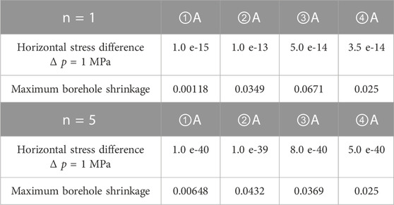
TABLE 5. The pre-coefficient A and the exponent n (Layer No. 3), in the case of n = 1 and n=5.

When the dislocation mechanism is dominant (n=5), the first simulation with the assumed creep parameter A = 1.0 × 10⁻⁴⁰ was found with the calculated maximum borehole shrinkage of 0.00648 m; the second simulation with the assumed creep parameter A = 1.0 × 10⁻³⁹, the calculated maximum borehole shrinkage of 0.0432 m; the third simulation with the assumed creep parameter A = 8.0 × 10⁻⁴⁰, the calculated maximum borehole shrinkage of 0.0369 m; finally, the fourth simulation with the assumed creep parameter A = 5.0 × 10⁻⁴³, the calculated maximum borehole shrinkage of 0.025 m, which is consistent with the actual reaming amount (Table 5).

In cases of varied horizontal stress differences, the differential stresses were set as 1 MPa, 5 MPa, 10 MPa, and 15 MPa, respectively. When the horizontal stress difference is 1 MPa, the pressure solution mechanism is dominant (n = 1), and A = 3.5 × 10⁻¹⁴, the near-wellbore stress field after reaming (Figure 11A) shows the near-wellbore Mises stress is about 1 MPa and the differential stress in the far field is 1 MPa. The borehole shrinkage after reaming is shown in Figure 11B—after 3 days, the maximum shrinkage deformation is located at the horizontal endpoint of the wellbore, where the wellbore diameter restores to the original value. When the dislocation mechanism is dominant (n=5) and A = 4.6 × 10⁻⁴⁰, the post-reaming near-wellbore stress field distribution (Figure 11C) reveals that the Mises stress around the wellbore is about 2 MPa and the differential stress in the far field is 1 MPa. Moreover, Figure 11D shows the borehole shrinkage after reaming. After 3 days, the maximum shrinkage deformation is evenly distributed around the wellbore—the borehole returns to its original diameter. The case of the horizontal stress difference of 1 MPa indicates that the creep deformation distribution around the well is relatively uniform and the maximum creep deformation occurs around the borehole wall.

FIGURE 11

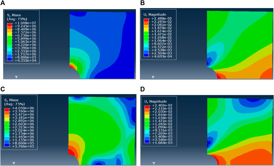
FIGURE 11. (A–D) Mises stress and displacement of borehole shrinkage after reaming (ΔP = 1 MPa, n = 1). Mises stress and displacement of borehole shrinkage after reaming (ΔP = 1 MPa, n = 5)

The simulations in the case of the horizontal stress difference of 5 MPa are presented below. When the pressure solution mechanism is dominant (n = 1), the first simulation with the creep parameter A = 1.0 × 10⁻¹⁵ led to the maximum borehole shrinkage of 0.0023 m; the second simulation with the creep parameter A = 8.0 × 10⁻¹⁴, the maximum borehole shrinkage of 0.09826 m; the third simulation with the creep parameter A = 4.0 × 10⁻¹⁴, the maximum borehole shrinkage of 0.05532 m; the fourth simulation with the creep parameter A =2.2 × 10⁻¹⁴, the maximum borehole shrinkage of 0.025 m, which is consistent with the actual borehole reaming amount. See Table 6 for specific parameters and their values.

TABLE 6

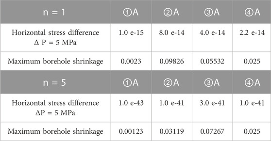
TABLE 6. The pre-coefficient A and the exponent n (Layer No. 3), in the case of n = 1 and n=5.

When the dislocation creep mechanism is dominant (n = 5), the first simulation with the creep parameter A = 1.0 × 10⁻⁴³ gave the maximum borehole shrinkage of 0.00123 m; the second simulation with the creep parameter A = 1.0 × 10⁻⁴¹, the maximum borehole shrinkage of 0.03119 m; the third simulation with the creep parameter A = 3.0 × 10⁻⁴¹, the maximum borehole shrinkage of 0.07267 m; the fourth simulation with the creep parameter A = 1.0 × 10⁻⁴¹, the maximum borehole shrinkage of 0.025 m, which is consistent with the actual borehole reaming result (Table 6).

In the case of the horizontal stress difference of 5 MPa, the dominance of the pressure solution mechanism (n = 1) and A = 2.2 ×10⁻¹⁴, the simulated post-reaming near-wellbore stress field distribution (Figure 12A) shows that the Mises stress around the wellbore is about 3–20 MPa and the differential stress in the far field is 5 MPa. Furthermore, the wellbore shrinkage after reaming is illustrated in Figure 12B—after 3 days, the maximum shrinkage deformation is located at the horizontal endpoint of the wellbore, where the wellbore returns to the original diameter. When the dislocation creep mechanism is dominant (n = 5) and A = 1.0 × 10⁻⁴¹, the simulated post-reaming stress field distribution around the borehole (Figure 12C) shows that the near-wellbore Mises stress is about 2–10 MPa and the differential stress in the far field is 5 MPa. Furthermore, 3 days after reaming, the maximum shrinkage deformation is evenly distributed around the wellbore and the wellbore returns to the original radius, as is made evident by Figure 12D. In other words, with the horizontal stress difference of 5 MPa, the creep deformation distribution is relatively uniform when the dislocation mechanism is dominant. According to the Mises stress distribution, the stress difference is 4 MPa in the far distance, in the case of the dominance of the pressure solution mechanism; however, it is mostly 6 MPa when the dislocation creep mechanism is dominant.

FIGURE 12

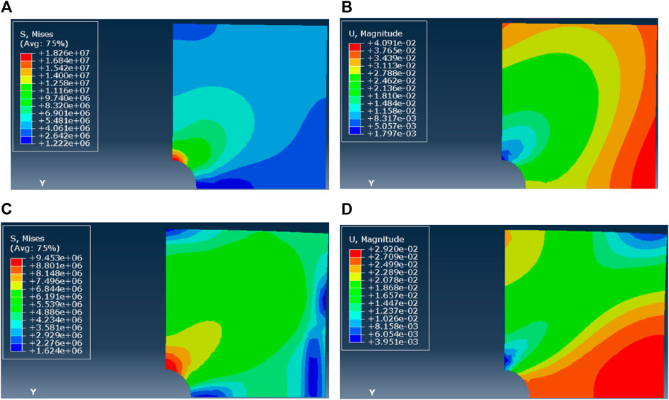
FIGURE 12. (A–D) Mises stress and displacement of borehole shrinkage after reaming (ΔP = 5 MPa, n = 1). Mises stress and displacement of borehole shrinkage after reaming (ΔP = 5 MPa, n = 5)

The simulations in the case of the horizontal stress difference of 10 MPa are presented below. When the pressure solution mechanism is dominant (n = 1), the first simulation with the creep parameter A = 1.0 × 10⁻¹⁵ led to the maximum borehole shrinkage of 0.00237 m; the second simulation with the creep parameter A = 3.0 × 10⁻¹⁴, the maximum borehole shrinkage of 0.08484 m; the third simulation with the creep parameter A = 4.0 × 10⁻¹⁴, the maximum borehole shrinkage of 0.05689 m; the fourth simulation with the creep parameter A =1.2 × 10⁻¹⁴, the maximum borehole shrinkage of 0.025 m, which is consistent with the actual borehole reaming amount. See Table 7 for specific parameters and their values.

TABLE 7

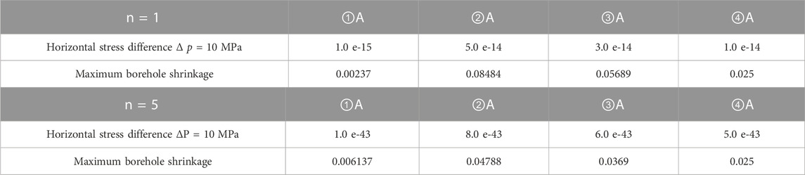
TABLE 7. The pre-coefficient A and the exponent n (Layer No. 3), in the case of n = 1 and n=5.

When the dislocation creep mechanism is dominant (n = 5), the first simulation with the creep parameter A = 1.0 × 10⁻⁴³ gave the maximum borehole shrinkage of 0.006137 m; the second simulation with the creep parameter A = 8.0 × 10⁻⁴³, the maximum borehole shrinkage of 0.04788 m; the third simulation with the creep parameter A = 6.0 × 10⁻⁴¹, the maximum borehole shrinkage of 0.0369 m; the fourth simulation with the creep parameter A = 5.0 × 10⁻⁴³, the maximum borehole shrinkage of 0.025 m, which is consistent with the actual borehole reaming result (Table 7).

In the case of the horizontal stress difference of 10 MPa, the dominance of the pressure solution mechanism (n = 1) and A = 1.0 ×10⁻¹⁴, the simulated post-reaming near-wellbore stress field distribution (Figure 13A) shows that the Mises stress around the wellbore is about 3–30 MPa and the differential stress in the far field is 10 MPa. Furthermore, the wellbore shrinkage after reaming is illustrated in Figure 13B—after 3 days, the maximum shrinkage deformation is located at the horizontal endpoint of the wellbore, where the wellbore returns to the original diameter. When the dislocation creep mechanism is dominant (n = 5) and A = 5.0 × 10⁻⁴³, the simulated post-reaming stress field distribution around the borehole (Figure 13C) shows that the near-wellbore Mises stress is about 3–17 MPa and the differential stress in the far field is 10 MPa. Furthermore, 3 days after reaming, the maximum shrinkage deformation is evenly distributed around the wellbore and the wellbore returns to the original radius, as is made evident by Figure 13D. In other words, with the horizontal stress difference of 10 MPa, the creep deformation distribution is relatively uniform when the dislocation mechanism is dominant. According to the Mises stress distribution, the stress difference is 6–10 MPa in the far distance, in the case of the dominance of the pressure solution mechanism; however, it is mostly 8–12 MPa when the dislocation creep mechanism is dominant.

FIGURE 13

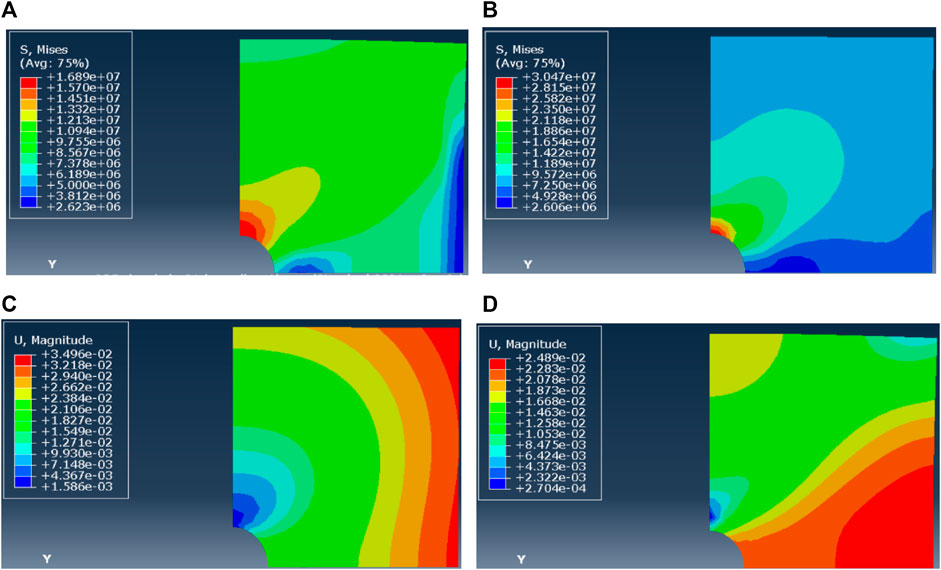
FIGURE 13. (A–D) Mises stress and displacement of borehole shrinkage after reaming (ΔP = 10 MPa, n = 1). Mises stress and displacement of borehole shrinkage after reaming (ΔP = 10 MPa, n = 5)

The simulations in the case of the horizontal stress difference of 15 MPa are presented below. When the pressure solution mechanism is dominant (n = 1), the first simulation with the creep parameter A = 1.0 × 10⁻¹⁵ led to the maximum borehole shrinkage of 0.00383 m; the second simulation with the creep parameter A = 3.0 × 10⁻¹⁴, the maximum borehole shrinkage of 0.09291 m; the third simulation with the creep parameter A = 2.0 × 10⁻¹⁴, the maximum borehole shrinkage of 0.05814 m; the fourth simulation with the creep parameter A =1.2 × 10⁻¹⁴, the maximum borehole shrinkage of 0.025 m, which is consistent with the actual borehole reaming amount. See Table 8 for specific parameters and their values.

TABLE 8

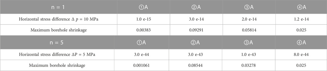
TABLE 8. The pre-coefficient A and the exponent n (Layer No. 3), in the case of n = 1 and n=5.

When the dislocation creep mechanism is dominant (n = 5), the first simulation with the creep parameter A = 3.0 × 10⁻⁴⁴ gave the maximum borehole shrinkage of 0.01061 m; the second simulation with the creep parameter A = 3.0 × 10⁻⁴³, the maximum borehole shrinkage of 0.08544 m; the third simulation with the creep parameter A = 1.0 × 10⁻⁴³, the maximum borehole shrinkage of 0.03278 m; the fourth simulation with the creep parameter A =8.0 × 10⁻⁴⁴, the maximum borehole shrinkage of 0.025 m, which is consistent with the actual borehole reaming result (Table 8).

When the horizontal stress difference is 15 MPa and the pressure solution mechanism is dominant, A= 1.2×10⁻¹⁴, n=1. Figure 14A shows the stress field distribution around the borehole wall after reaming. The Mises stress around the borehole is about 4–40 MPa, and the differential stress in the far field is 15 MPa. Figure 14B shows the shrinkage of the borehole wall after reaming. After 3 days, the maximum deformation of shrinkage is located at the end point of the horizontal direction of the borehole and is restored to the original borehole radius. When the dislocation mechanism is dominant, A = 8.0×10⁻⁴³, n=5. Figure 14C shows the stress field distribution around the borehole wall after reaming. The Mises stress around the borehole is about 5–24 MPa, and the differential stress in the far field is 15 MPa. Figure 14D shows the wellbore shrinkage after reaming. After 3 days, the maximum deformation position of shrinkage is at the end point in the horizontal direction of the wellbore, and it is restored to the original wellbore radius position. From the horizontal difference stress of 15 MPa, when the dislocation mechanism is dominant, the creep deformation distribution is no longer uniform. From the Mises stress distribution, when the pressure solution mechanism is dominant, the stress difference in the area far from the well periphery is 10–12 MPa, while the dislocation mechanism is dominant, the stress difference in the area far from the well periphery is 12–15 MPa.

FIGURE 14

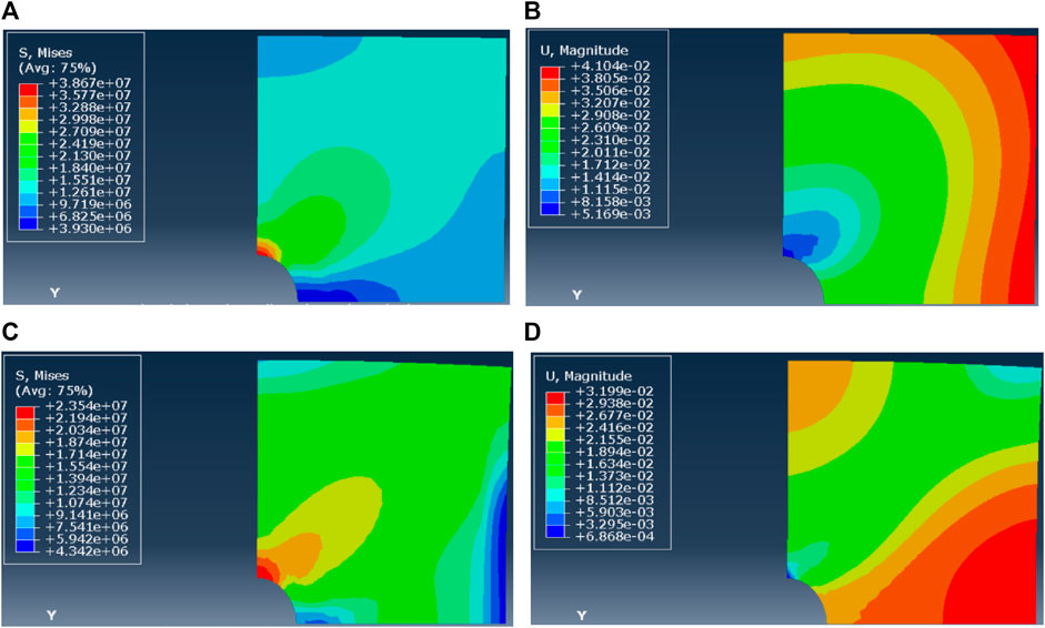
FIGURE 14. (A–D) Mises stress and displacement of borehole shrinkage after reaming (ΔP = 15 MPa, n = 1). Mises stress and displacement of borehole shrinkage after reaming (ΔP = 15 MPa, n = 5)

Layer No. 3 is 1,000 m deeper than Layer No. 2 and with the deeper burial and elevated formation temperature, creep is enhanced. Hence, compared with Layer No. 2, the creep shrinkage deformation of Layer No. 3 is larger for the same time, which means larger reaming sizes are required. Our inversion shows that the creep pre-coefficient of Layer No. 3 is always higher than that of Layer No. 2, regardless of the dominance of the pressure solution and dislocation creep mechanisms.

Figures 15A,B show the correlations between the creep pre-coefficient and horizontal stress difference, in cases of the dominance of the pressure solution creep mechanism (n = 1) and dislocation creep mechanism (n = 5), respectively. It can be seen that as the formation depth increases, the temperature rises and the formation rheology enhances. Under such circumstances, a larger reaming size is required. The inverted creep parameter of Layer No. 3 (5,525–6,543 m) is larger than that of Layer No. 2 (4,833–5,525 m). The actual principal stress difference in salt layers is directly related to the horizontal in situ stress, vertical stress, and stress attributed to the drilling fluid column in the wellbore. When the horizontal stress difference is 1 MPa, 5 MPa, 10 MPa, and 15 MPa, respectively, and the pressure solution mechanism is dominant (n = 1), the creep pre-coefficient of Layer No. 2 varies from 7 × 10⁻¹⁵ to 2.6 × 10⁻¹⁴ at the same order of magnitude. However, under the dominance of the dislocation creep mechanism (n = 5), the creep pre-coefficient ranges from 7 × 10⁻⁴⁴ to 6.3 × 10⁻⁴¹ by a span of 4 orders of magnitude, corresponding to the horizontal stress differences of 1, 5, 10, and 15 MPa. For Layer No. 3 with the dominant pressure solution mechanism (n = 1), the creep parameter varies from 8 × 10⁻¹⁵ to 3.5 × 10⁻¹⁴ at the same order of magnitude; yet, it ranges from 8 × 10⁻⁴⁴ to 4.6 ×10⁻⁴⁰ by a span of 5 orders of magnitude, in the case of the dominance of the dislocation creep mechanism.

FIGURE 15

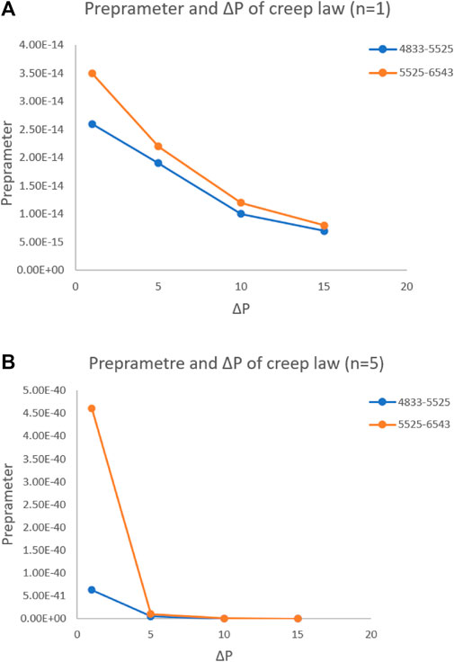
FIGURE 15. (A) Creep pre-coefficient vs horizontal stress difference (n = 1). (B). Creep pre-coefficient vs horizontal stress difference (n = 5)

5 Conclusions and suggestions

Based on the reaming performance and borehole situation of an actual well, the creep shrinkage of the wellbore under different horizontal stress differences and the distribution of the Mises stress representing the principal stress difference were computed via the theoretical and numerical simulation analyses, in cases of the dominance of the dislocation creep and pressure solution creep mechanisms, respectively. With the same creep deformation and yet different horizontal stress differences, the creep pre-coefficient of the dislocation creep mechanism varies by 4–5 orders of magnitude, while that of the pressure solution creep mechanism changes by 1–2 orders of magnitude.

With the increases in the depth, the formation temperature grows and formations become more movable. Hence, the reaming size can be expanded. It is obvious that the inverted creep parameters of Layer No. 3 are larger than those of Layer No. 2. Moreover, the actual Mises stress (reflecting the magnitude of the principal stress difference) in salt layers is directly related to the horizontal in situ stress, vertical stress, and stress attributed to the drilling fluid column in the wellbore. The creep pre-coefficient varies by more than one order of magnitude, in the case of the dominant pressure solution mechanism with n=1, while that spans several orders of magnitude, under the dominance of the dislocation mechanism with n=5.

The numerical simulation version based on reaming while drilling and field data is an effective method to determine the creep law of composite salt layers. It can serve as an effective supplement to other test methods like laboratory experiments (with various limitations). The creep law and parameters of specific formations can be inverted, according to the specific horizontal stress difference, drilling fluid density, and post-reaming deformation and the overall creep and wellbore stability of composite salt layers can also be effectively predicted. However, in terms of what deformation mechanisms control creep mechanisms of specific salt layers, further studies with a more comprehensive methodology are still needed.

Author contributions

All authors listed have made a substantial, direct, and intellectual contribution to the work and approved it for publication. All authors contributed to the article and approved the submitted version.

Funding

The research is funded by National Natural Science Foundation of China (No. 52174011) and Research on reaming while drilling and open hole overlapping suspension technology of expansion pipe (No. 2021DJ4102).

Conflict of interest

Authors ZC, WZ, XC were employed by CNPC Engineering Technology R&D Company Limited.

The remaining authors declare that the research was conducted in the absence of any commercial or financial relationships that could be construed as a potential conflict of interest.

Publisher’s note

All claims expressed in this article are solely those of the authors and do not necessarily represent those of their affiliated organizations, or those of the publisher, the editors and the reviewers. Any product that may be evaluated in this article, or claim that may be made by its manufacturer, is not guaranteed or endorsed by the publisher.

References

Chen, S., Zhang, H., and Yin, G. (2014). Study on prediction of sticking time for creep shrinkage of gypsum salt rock. Tech. Superv. Petroleum Industry 30 (10), 32–35.

Google Scholar

Farmer, I., and Gilbert, M. (1984). Dependent strength reduction of rock salt. The first Conference on the Mechanical behavior of salt, 4–18.

Google Scholar

Fossum, A. F., and Fredrich, J. T. (2002). Salt mechanics primer for near-salt and sub-salt deepwater Gulf of Mexico field developments SANDIA REPORT sand2002–2063.

Google Scholar

Huang, R., and Deng, J. (2000). Testing study on mechanical property of thenardite rock salt. Chin. J. Rock Mech. Eng. (S1), 1000–6915.

Google Scholar

Hunsche, U., and Hampel, A. (1999). Rock salt - the mechanical properties of the host rock material for a radioactive waste repository. Eng. Geol. 52 (3-4), 271–291. doi:10.1016/s0013-7952(99)00011-3

CrossRef Full Text | Google Scholar

Hunsche, U., Schulze, O., Walter, F., and Plischke, I. (2003). Projekt gorleben: Thermomechanisches verhalten von Salzgestein.

Google Scholar

Jiang, L., Yang, C., and Wu, W. (2006). Experimental study on short-term strength and deformation properties of rock salts. Chin. J. Rock Mech. Eng. 25, 3104–3109.

Google Scholar

Li, S., Li, F., Liu, Y., and Lu, Y. (2019). Deformation mechanism and numerical simulation of interface dislocation in composite salt gypsum layer [J]. Petroleum Sci. Bull. 12 (4), 390–402.

Google Scholar

Li, S., and Urai, J. L. (2016). Rheology of rock salt for salt tectonics modeling. Petroleum Sci. Nov 13, 712–724. doi:10.1007/s12182-016-0121-6

CrossRef Full Text | Google Scholar

Li, Y., Yang, C., Daemen , J. J. k., Yin, X., and Chen, F. (2009). A new Cosserat-like constitutive model for bedded salt rocks. Int. J. Numer. Anal. methods geomechanics 33 (15), 1691–1720. doi:10.1002/nag.784

CrossRef Full Text | Google Scholar

Liang, C., Liu, J., Chen, Z., Lu, G., Lyu, C., and Ren, Y. (2022). Study on salt rock characteristics of wellbore under high temperature and high pressure. J. Porous Media 25 (3), 1–19.

CrossRef Full Text | Google Scholar

Liang, W., and Zhao, Y. (2004). The viscosity coefficient of rheological formation and its influential factor. Chin. J. Rock Mech. Eng. 23 (3), 391–394.

Google Scholar

Lin, H., Deng, J., and Xu, J. (2018). Borehole shrinkage mechanisms and countermeasure analysis of composite salt-gypsum layer. Fault-Block Oil Gas Field 25 (06), 793–798.

Google Scholar

Lin, Y., Zeng, D., and Shi, T. (2005). Inversion algorithm for creep laws of salt rocks. Acta Pet. Sin. 05, 115–118.

Google Scholar

Moosavi, M., Jafari, M., and Rassouli, F. (2009). “Investigation on creep behavior of salt rock under high temperature with impression technique,” in Proceedings of the 2009 international symposium on rock mechanics (China: Hong Kong).

Google Scholar

Orlic, B., Wollenweber, J., and Geel, C. (2019). “Formation of a sealing well barrier by the creep of rock salt: Numerical investigations,” in Proceedings of the 53rd US rock mechanics/geomechanics symposium, F.

Google Scholar

Orozco, S., Pino, J., and Paredes, M. (2018). “Managing creep closure in salt uncertainty while drilling,” in Proceedings of the 52nd US rock mechanics/geomechanics symposium, F, 2018 [C] (American Rock Mechanics Association).

Google Scholar

Renard, F., Bernard, D., Thibault, X., and Boller, E. (2004). Synchrotron 3D microtomography of Halite aggregates during experimental pressure solution creep and evolution of the permeability. Geophys. Res. Lett. 31, L07607. doi:10.1029/2004GL019605

CrossRef Full Text | Google Scholar

Spiers, C. J., Schutjens, P. M. T. M., Brzesowsky, R. H., Peach, C. J., Liezenberg, J. L., and Zwart, H. J. (1990). “Experimental determination of constitutive parameters governing creep of rocksalt by pressure solution,” in Deformation mechanisms, rheology and tectonics. Editors R. J. Knipe, and E. H. Rutter (Geol. Soc. London, Spec. Publ.), 54, 215–227.

CrossRef Full Text | Google Scholar

Urai, J. L., Spiers, C. J., Zwart, H. J., and Lister, G. S. (1986). Weakening of rock salt by water during long-term creep. Nature 324, 554–557. doi:10.1038/324554a0

PubMed Abstract | CrossRef Full Text | Google Scholar

Wang, Y., Zhu, C., He, M. C., Wang, X., and Le, H. L. (2022). Macro-meso dynamic fracture behaviors of Xinjiang marble exposed to freeze thaw and frequent impact disturbance loads: A lab-scale testing. Geomechanics Geophys. Geo-Energy Geo-Resources 8 (5), 154. doi:10.1007/s40948-022-00472-5

CrossRef Full Text | Google Scholar

Wawersik, W. R., and Zimmerer, D. J. (1994). “Triaxial creep measurements on rock salt from the jennings dome, technical report,” in Louisiana, borehole LA-1, core #8*, geomechanics department 61 I 7 (Albuquerque: Sandia National Laboratories). AM 8 71 85-0 751.

Google Scholar

Weidinger, P., Hampel, A., Blum, W., and Hunsche, U. (1997). Creep behaviour of natural rock salt and its description with the composite model. Mater. Sci. Eng. 234, 646–648. doi:10.1016/s0921-5093(97)00316-x

CrossRef Full Text | Google Scholar

Zeng, D., Lin, Y., and Lu, Y. (2012). Numerical Simulation of hole creep shrinkage for composite rock salt layers. Chin. J. Geomechanics 18 (02), 158–164.

Google Scholar