High-resolution imaging of a coal seam based on quasi-2D TEM inversion

1 Introduction

The transient electromagnetic (TEM) method is a geophysical exploration tool based on electromagnetic induction theory (Stacey, 1976). The electromagnetic pulse signals from a loop source diffuse into the earth to underground anomalies and eventually induce a secondary electromagnetic field that can be observed by a receiver. Secondary field signal processing is employed for the discovery of subsurface minerals or to address geological problems (Fitterman and Stewart, 1986; Fountain et al., 2005; Jiang et al., 2019). This method has been widely used in coal mine water damage detection (Si et al., 2020), hydrogeological surveys (Danielsen et al., 2003), engineering investigations (Hui et al., 2021), and mineral exploration (Yang and Oldenburg, 2012) owing to its flexible working device, high efficiency, and high resolution.

The TEM data must be interpreted to obtain the underground electrical structure. Early TEM data interpretation methods were approximations based on the smoke-ring theory (Nabighian, 1979; Yang et al., 2016). By defining the apparent resistivity and calculating the diffusion depth (apparent depth) of the smoke ring, a relatively approximate pseudosection map of the apparent resistivity is obtained. These results are inaccurate and are suitable only for preliminary interpretation. Different definitions of the apparent resistivity will lead to large differences in the inversion results. To obtain a more accurate geoelectric model, it is necessary to carry out inversion calculations for TEM data. At present, the mainstream inversion methods are the damped least-squares method (Huang and Palacky, 2010) and the Occam inversion method (Constable et al., 1987), which introduces the regularization of model constraints. By adding a penalty function term to the objective function, different optimizers are used to minimize the difference between the observation data and the model response, and a stable and unique solution can be obtained. Regularization increases the constraint information or prior information of the inversion parameter model, reduces the multiplicity of inversion solutions, and enhances the stability of the inversion. The least squares inversion method requires a good initial guess, and the inversion results easily fall into local minima. The Occam inversion method adds model smoothing constraints to the objective function, which make the stratigraphic interface unclear in the inversion results. These 1D inversion methods are all based on the single-point horizontal layered model, and the inversion resistivity is prone to lateral discontinuity (Farquharson and Oldenburg, 1993; Christensen et al., 2009). In the past decades, the demand of accurate three-dimensional (3D) interpretation of TEM data and the rapid development of computation devices promotes researches on the development of 3D forward modeling and inversion (Liu et al., 2019; Ren et al., 2018; Zhang et al., 2021). Due to the time-consuming inversion of 3D TEM data, their practical applications are limited. Considering the relatively continuous distribution of underground electrical properties in sedimentary strata, it is natural to adopt the laterally constrained inversion method (LCI). The LCI method is a quasi-2D inversion method, which integrates the data of a single profile and multiple measuring points and applies lateral constraints to achieve a relatively continuous resistivity profile.

LCI was first proposed by Auken, Thomsen, and Sorenson (2000) and applied to direct current (DC) data inversion. The main idea is to use a transversely constrained sparse matrix to transform a single-point inversion into a collective inversion of multiple measuring points, to ensure the transverse continuity of the inversion profile. Santos (2004) used this method to obtain the high-quality EM34 inversion profile; Auken and Christiansen (2004) optimized the 2D LCI inversion and segmented the inversion of resistivity data by calculating the Jacobi matrix through the Broyden approximation; Siemon et al. (2009) used the LCI inversion method to process helicopter survey data, which effectively improved the transverse continuity of the profile. Auken et al. (2008) processed TEM data in a paleochannel survey using the LCI technique; Cai et al. (2014) proposed the weighted laterally constrained inversion (WLCI), which was used for inversion calculation of frequency-domain airborne EM data. The effectiveness of the WLCI was verified through inversion processing of theoretical and measured data and comparison with conventional 1D inversion results. Yin et al. (2016) used the WLCI method to invert airborne TEM data. Zhang et al. (2022) used WLCI on time-domain electromagnetic data. To increase the speed of the inversion computation, Lu et al. (2022) developed an analytical technique based on the chain rule to calculate the Jacobi matrix. They then used the WLCI approach to invert four induced polarization parameters from airborne TEM data.

In view of the relatively continuous underground electrical structure of adjacent measuring points in sedimentary strata, we adopt different lateral resistivity constraints and layer interface depth constraints based on the idea of horizontal constraints. Compared with conventional inversion methods, this method effectively improves the vertical resolution of the inversion layer interface. Finally, field data from Inner Mongolia are inverted to test the practicality of the method.

2 Methodology

2.1 Forward modeling theory

To generate 1D TEM forward responses, we first must calculate the frequency domain responses and then translate them to the time domain via Fourier transform (Johansen and Sorensen, 1979). Suppose there are n levels in the strata, and each layer has a conductivity (σ) and thickness (h), as ${\sigma }_1,h_1;{\sigma }_2,h_2;\cdots ;{\sigma }_n,h_n;h_n\to \infty$. When calculating the TEM responses in the frequency domain, we simulate a transmitting loop by dividing the loop into a series of current segments, with each segment being treated as an electric dipole. Using the Dirac function integration, the analytical expression in the frequency domain for the vertical component ${\mathbf{B}}_z$ of the electromagnetic field at any point on the surface is

${\mathbf{B}}_z\left(x,y,\omega \right)={\displaystyle \sum _{j=1}^L}\frac{{\mathbf{P}}_{E_j}}{2\pi }{\mu }_0\sin {\phi }_j{\int }_0^{\infty }\frac{{\lambda }^2}{\lambda +u_1/R_1}{J}_1\left(\lambda r_j\right)\mathrm{d}\lambda (1)$

where $L$ is the number of electric dipoles, ${\mathbf{P}}_{E_j}$ is the magnetic moment of the jth electric dipole, ${\mu }_0$ is the magnetic conductivity of vacuum, ${\phi }_j$ is the angle between the jth electric dipole and the measuring point, $J_1\left(\lambda r_j\right)$ is the first-order Bessel function, and $r_j$ is the distance between the jth electric dipole and the measuring point, where $R_1=\mathrm{c}\mathrm{t}\mathrm{h}\left[u_1{h}_1+\mathrm{a}\mathrm{r}\mathrm{c}\mathrm{t}\mathrm{h}\left(u_1/u_2\right)\mathrm{c}\mathrm{t}\mathrm{h}\left(u_2{h}_2+\cdots +\mathrm{a}\mathrm{r}\mathrm{t}\mathrm{c}\mathrm{h}{u}_{n-1}/u_n\right)\right]$ and $u_j=\sqrt{{\lambda }^2+k_j^2},k_j^2=-\mathrm{i}\omega {\mu }_0{\sigma }_j$, $\omega$ is angular frequency. Finally, the time-domain response of any measurement point on the surface of the loop source can be obtained by cosine transformation (Guptasarma, 1982) of Eq. (1).

2.2 1D inversion theory

We use regularization to address the ill-posed nature of the TEM inversion by minimizing the l₂-norm-based objective function, i.e.,

${\mathbf{U}}_m=R+{\mu }^{-1}\left\{{‖\mathbf{W}{\mathbf{d}}_{obs}-\mathbf{W}\mathbf{F}\left[\mathbf{m}\right]‖}^2-{\mathbf{X}}_{\infty }^2\right\}(2)$

where $\mu$ is the trade-off parameter, ${\mathbf{d}}_{obs}$ is the observed data, $\mathbf{F}$ is the 1D forward operator, and $\mathbf{m}$ represents the inversion parameters of the model. ${\mathbf{X}}_{\infty }^2$ is the expected misfit. Here, we adopt the covariance matrix to obtain the misfit between the forward response and observed data, which is represented as

$\mathbf{W}=\mathrm{d}\mathrm{i}\mathrm{a}\mathrm{g}\left\{\frac{1}{{\epsilon }_1},\frac{1}{{\epsilon }_2},\cdots ,\frac{1}{{\epsilon }_j},\frac{1}{{\epsilon }_{\mathrm{M}}}\right\}(3)$

where ${\epsilon }_j$ is the standard deviation of the jth observed data, and $M$ is the number of observed data. The roughness function represents the roughness of the inverse model, for which the matrix expression is

$R={‖\mathbf{P}\cdot \mathbf{m}‖}^2(4)$

where P is the unit matrix consisting of 1 and −1, which can be expressed as

$\mathbf{P}=\left[\begin{array}{ccccc}0& & & & 0\\ -1& 1& & & \\ & -1& 1& & \\ & & \cdots & \cdots & \\ & 0& & -1& 1\end{array}\right](5)$

To minimize ${\mathbf{U}}_m$, we can set $\nabla {\mathbf{U}}_m$ equal to zero; then we have the iterative equation,

$\left[{\left(\mathbf{W}\mathbf{G}\right)}^{\mathrm{T}}\mathbf{W}\mathbf{G}+\mu {\mathbf{P}}^{\mathrm{T}}\mathbf{P}\right]\Delta {\mathbf{m}}_q={\left(\mathbf{W}\mathbf{G}\right)}^{\mathrm{T}}\mathbf{W}\mathbf{\Delta }{\mathit{d}}_{\mathit{q}}(6)$

where $\mathbf{G}$ is the Jacobian matrix of sensitivities. Its elements can be expressed as

${\mathbf{G}}_{ij}=\frac{\partial F_i\left[\mathbf{m}\right]}{\partial {\mathbf{m}}_j}(7)$

By solving Eq. 6 and minimizing the misfit between the predicted data and the observed data $\Delta d_q$, we obtain the inversion model update $\Delta {\mathbf{m}}_q$ of the qth iteration; then we can update the model via ${\mathbf{m}}^q={\mathbf{m}}^{q-1}+s\delta \mathbf{m}$. The value of $s$ is set initially to one. We adopt a cooling approach (Haber and Schwarzbach, 2014) for selecting $\mu$ in our inversions.

2.3 WLCI inversion theory

2.3.1 Resistivity lateral constraint

To improve the lateral continuity of the resistivity inversion of adjacent measurement points, we begin with the LCI inversion proposed by Auken and Christiansen (2004) and include the differences between geoelectric parameters of adjacent measurement points as constraint terms to the objective function. Assuming that

${\mathbf{R}}_p\mathbf{m}-{\mathbf{e}}_{rp}=0(8)$

Where ${\mathbf{e}}_{rp}$ represents the different model parameters of adjacent points, and ${\mathbf{R}}_p$ is the horizontal constraint matrix, which is a sparse matrix with the values 1 and −1, i.e.,

${\mathbf{R}}_p={\left[\begin{array}{cccccccccc}1& 0& \cdots & 0& -1& 0& \cdots & 0& 0& 0\\ 0& 1& 0& \cdots & 0& -1& 0& \cdots & 0& 0\\ ⋮& & & & & ⋮& & & & ⋮\\ 0& 0& 0& \cdots & 0& 1& 0& \cdots & 0& -1\end{array}\right]}_{\mathrm{S}\times \mathrm{T}}(9)$

where $\mathrm{S}=\left(M-1\right)\times \left(2N-1\right),\mathrm{T}=M\times \left(2N-1\right)$, $M$ is the number of the data receiver, and $N$ is the number of layers. Subtracting ${\mathbf{R}}_p{\mathbf{m}}_0$ from both sides of Eq. (8), we have

${\mathbf{R}}_p\Delta \mathbf{m}=\Delta {\mathbf{r}}_p+{\mathbf{e}}_{rp}(10)$

where $\mathbf{\Delta }{\mathit{r}}_{\mathit{p}}=-{\mathbf{R}}_p{\mathbf{m}}_0,\Delta {\mathbf{m}}_0=\mathbf{m}-{\mathbf{m}}_0$.

We adopt the horizontal constrained factor to accomplish WLCI and adjust the horizontal smoothness of each layer. Thus, Eq. (8) can be written as

${\mathbf{R}}_p^{\prime }\Delta \mathbf{m}=\Delta {\mathbf{r}}_p^{\prime }+{\mathbf{e}}_{rp}^{\prime }(11)$

Where ${\mathbf{R}}_p^{\prime }={\mathbf{W}}_p{\mathbf{R}}_p,\Delta r_{\mathrm{p}}^{\prime }=-{\mathbf{R}}_p^{\prime }{\mathbf{m}}_0,{\mathbf{e}}_{rp}^{\prime }={\mathbf{W}}_p{\mathbf{e}}_{rp}$. ${\mathbf{W}}_p$ is the horizontal constraint weighting matrix, which equals to the horizontal constrained factor multiplied by the matrix ${\mathbf{R}}_p$. The inversion’s smoothness is determined by the constrained factor’s value, which is dependent on the smoothness of the parameters and the actual requirements.

2.3.2 Depth and layer interface constraints

The depth of the layer interfaces must be constrained to ensure the smoothness and continuity between the layer interfaces of the multilayer model (Auken and Christiansen, 2004). We have

${\mathbf{R}}_t\mathbf{m}-{\mathbf{e}}_{rt}=0(12)$

Where ${\mathbf{e}}_{rt}$ is the depth difference between each layer of adjacent points, and ${\mathbf{R}}_t$ is the depth constraint matrix, written as

${\mathbf{R}}_t={\left[\begin{array}{cccccccccccc}\cdots & 0& \cdots & 0& 1& 0& 0& \cdots & 0& \cdots & & \\ \cdots & 0& \cdots & 0& \frac{h_{k,1}}{t_{k,2}}& \frac{h_{k,2}}{t_{k,2}}& 0& \cdots & 0& \cdots & & \\ & ⋮& ⋮& ⋮& ⋮& & & & & & & \\ \cdots & 0& \cdots & 0& \frac{h_{k,1}}{t_{k,N-1}}& \frac{h_{k,2}}{t_{k,N-1}}& \frac{h_{k,3}}{t_{k,N-1}}& \cdots & \frac{h_{k,N-1}}{t_{k,N-1}}& \cdots & & \\ \cdots & 0& \cdots & 0& -1& 0& 0& \cdots & 0& \cdots & \cdots & \\ \cdots & 0& \cdots & 0& -\frac{h_{k+\mathrm{1,1}}}{t_{k+\mathrm{1,2}}}& -\frac{h_{k+\mathrm{1,2}}}{t_{k+\mathrm{1,2}}}& 0& & \cdots & 0& \cdots & \\ & ⋮& ⋮& ⋮& ⋮& & & & & & & \\ \cdots & 0& \cdots & 0& -\frac{h_{k+\mathrm{1,1}}}{t_{k+1,N-1}}& -\frac{h_{k+\mathrm{1,2}}}{t_{k+1,N-1}}& -\frac{h_{k+\mathrm{1,3}}}{t_{k+1,N-1}}& \cdots & -\frac{h_{k+1,N-1}}{t_{k+1,N-1}}& \cdots & & \end{array}\right]}_{\mathrm{S}\times \mathrm{T}}(13)$

This is a sparse matrix composed of depth $t$ and thickness $h$, where $h_{i,j}$ and $t_{i,j}$ are the thickness and the depth, respectively, of the lower interface of the ith point at the jth layer, and $S=\left(M-1\right)\times \left(N-1\right),T=M\times \left(2N-1\right)$.

As mentioned in Section 2.3.1, we use a vertically constrained factor to adjust the continuity between the interfaces of each layer. Thus, Eq. (12) can be written as

${\mathbf{R}}_t^{\prime }\Delta \mathbf{m}=\Delta {\mathbf{r}}_t^{\prime }+{\mathbf{e}}_{rt}^{\prime }(14)$

Correspondingly, ${\mathbf{R}}_t^{\prime }={\mathbf{W}}_t{\mathbf{R}}_t,\Delta r_{\mathrm{t}}^{\prime }=-{\mathbf{R}}_t^{\prime }{\mathbf{m}}_0,{\mathbf{e}}_{rt}^{\prime }={\mathbf{W}}_t{\mathbf{e}}_{rt}$, where ${\mathbf{W}}_t$ is the vertically constrained weighting matrix.

2.4 WLCI inversion equation and least-squares solution

Combined with the 1D inversion theory described in Section 2.2, we obtain the WLCI inversion equation,

$\left[\begin{array}{c}\mathit{G}\\ {\mathit{R}}_{\mathit{p}}^{\mathit{\prime }}\\ {\mathit{R}}_{\mathit{t}}^{\mathit{\prime }}\end{array}\right]\Delta \mathbf{m}=\left[\begin{array}{c}\mathbf{\Delta }{\mathit{d}}_{\mathit{o}\mathit{b}\mathit{s}}\\ \mathbf{\Delta }{\mathit{r}}_{\mathit{p}}^{\mathit{\prime }}\\ \mathbf{\Delta }{\mathit{r}}_{\mathit{t}}^{\mathit{\prime }}\end{array}\right]+\left[\begin{array}{c}{\mathit{e}}_{\mathit{o}\mathit{b}\mathit{s}}\\ {\mathit{e}}_{\mathit{r}\mathit{p}}^{\mathit{\prime }}\\ {\mathit{e}}_{\mathit{r}\mathit{t}}^{\mathit{\prime }}\end{array}\right](15)$

Simplifying Eq. (15), we have

${\mathbf{W}}^{\prime }\Delta {\mathbf{m}}_q=\mathbf{\Delta }{\mathit{d}}_{\mathit{q}}\mathbf{+}\mathit{e}(16)$

where ${\mathbf{W}}^{\prime }$ is the coefficient matrix. Based on the 1D inversion theory, we obtain the following inversion equation:

$\left({{\mathbf{W}}^{\prime }}^{\mathbf{T}}{\mathbf{W}}^{\prime }+\mu \mathbf{P}\right)\Delta {\mathbf{m}}_q={{\mathbf{W}}^{\prime }}^{\mathbf{T}}\Delta {\mathit{d}}_{\mathit{q}}(17)$

To solve Eq. (17), in this study, we use singular value decomposition (SVD) for the coefficient matrix ${\mathbf{W}}^{\prime }$, such that we have

${\mathbf{W}}^{\prime }=\mathbf{D}\mathbf{\Lambda }{\mathbf{V}}^{\mathbf{T}}(18)$

Where $\mathbf{D}$ and $\mathbf{V}$ are the data matrix and parameters matrix, respectively, and $\mathbf{\Lambda }$ is the singular value matrix. Substituting Eq. (18) into Eq. (17), we have

$\Delta {\mathbf{m}}_q=\mathbf{V}{\left({\mathbf{\Lambda }}^2+\mu \mathbf{P}\right)}^{-1}\mathbf{\Lambda }{\mathbf{D}}^{\mathbf{T}}\Delta {\mathbf{d}}_q(19)$

The initial resistivity model for inversion is provided first in the actual inversion calculation, and then Eq. (19) is used to perform iterative calculations until the objective function satisfies the specifications.

3 Synthetic examples

We first established a tilted layered stratum model to verify the effectiveness of the inversion strategy. As shown in Figure 1, we designed two groups of typical three-layer models with low-resistivity (H-model) and high-resistivity (K-model) layers in the middle with different dip angles. The background resistivity is 100 Ω·m, of which the resistivity of the low-resistivity layer in the H-type model is 10 Ω·m, and the resistivity of the high-resistivity layer in the K-type model is 1,000 Ω·m. A rectangular loop is used for transmission, and the receiving points are located inside the loop with 20 m point spacing. The transmission current is 1 A, and the maximum sampling time is 10 ms. The dB/dt response data of each measuring point is obtained by forward modeling of the 1D model (Figure 2). In the inversion, we add 3% Gaussian white noise to the dB/dt of each time channel.

FIGURE 1

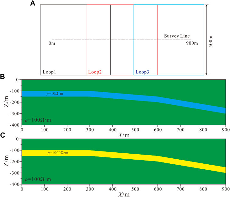
FIGURE 1. Synthetic model of inclined strata (A): Receiving and transmitting schematic. (B): H-type model. (C): K-type model.

FIGURE 2

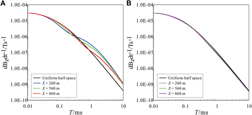
FIGURE 2. Single point decay curves of inclined strata models. (A): H-type model and corresponding uniform half space. (B): K-type model and corresponding uniform half space.

Figure 2 shows the TEM decay curves at different measuring points of the H and K models with different dip angles. When X = 260 m, the target layer is shallow, while when X = 860 m, the target layer is deep. In Figure 2A, the large amplitude of the low-resistivity layer at middle and late times indicates low-resistivity characteristics. With the increase in burial depth, the early amplitude tends to be consistent with the uniform half space, and the low-resistivity response is significantly delayed. Compared with the uniform half space in Figure 2B, when the high-resistivity layer is buried shallowly, the early time amplitude is small, reflecting the high resistivity. The late time amplitude tends to be consistent, exhibiting the characteristics of the background strata. With the increase in burial depth, the larger amplitude in the early time is the response of the background strata, the smaller amplitude in the middle stage is the response of the high-resistivity stratum, and the gradual increase in the late stage is close to the response of the background stratum, whereas the amplitude change is not evident.

Figure 3 shows the single-point inversion results of different inversion methods. The initial inversion models are all uniform half space models, and the initial resistivity of the model is 100 Ω·m. In the Occam inversion, the golden section method is used to select the damping factor. For the H-type tilt model, when the local stratum dip is small, the methods shown in Figure 3 better reflect the strata resistivity. When the strata dip is large, there is a significant difference between the resistivity of the shallow part and that of the real model. However, the head end and tail end of the WLCI single-point inversion curve are close to the real resistivity of the first and last layers, which is highly consistent with the actual low-resistivity layer. For the K-type tilt model, the conventional 1D inversion results are poor, the inversion depth of the high-resistivity layer has a large deviation from the given model, and the shallow resistivity is not consistent with the model resistivity. The amplitude characteristics of the high-resistivity layer in the single-point decay curve of the K-type model are not evident, and the horizontal continuity of the data is not considered in the conventional single-point 1D inversion, which is the main reason behind poor inversion results. As a quasi-2D inversion, the WLCI inversion better restores the resistivity distribution of inclined formations by considering the horizontal and vertical continuity of the data.

FIGURE 3

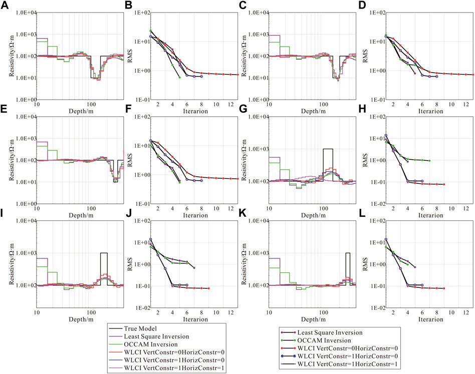
FIGURE 3. Single-point inversion results for different points. (A): Single-point inversion results at X = 260 m of H-type model. (B): The Root Mean Square (RMS) at X = 260 m of H-type model. (C): Single-point inversion results at X = 600 m of H-type model. (D): The RMS at X = 600 m of H-type model. (E): Single-point inversion results at X = 900 m of H-type model. (F): The RMS at X = 900 m of H-type model. (G): Single-point inversion results at X = 260 m of K-type model. (H): The RMS at X = 260 m of K-type model. (I): Single-point inversion results at X = 600 m of K-type model. (J): The RMS at X = 600 m of K-type model. (K): Single-point inversion results at X = 900 m of K-type model. (L): The RMS at X=900 m of K-type model.

Comparing the inversion results of different inversion methods in Figure 4, the conventional 1D and WLCI inversions reflect the electrical structure of the three underground layers. When the dip angle of the local layer is small, the conventional 1D inversion results efficiently reflect the low-resistivity layer in the H-type model relatively; however, the layer interface is rough, and the horizontal continuity is poor. In comparison to the least-squares inversion (Figure 4A), the resistivity continuity of the Occam inversion (Figure 4C) is slightly improved. The conventional 1D inversion has been unable to obtain a continuous high-resistivity layer for the K-type model. The inversion high-resistivity layer becomes thinner, and the resistivity decreases where the burial depth is large. When the dip angle of the local layer is large, the conventional 1D inversion results deviate significantly from the actual model. False anomalies appear in the shallow part of the H-type model (Figure 4A; Figure 4C), the resistivity of the inversion increases, and the layer becomes thicker where the low-resistivity layer is buried deeply. The high-resistivity layer is discontinuous and inconspicuous for the K-type model, and the inversion results can no longer represent the electrical characteristics of the actual formation. The resistivity obtained by the WLCI method is uniformly distributed laterally, and the layer interface is evident and continuous, which better reflects the electrical distribution characteristics of inclined strata. The inversion of the target layer is only slightly thicker than that of the actual model. For the strata with a small dip angle, the size of the constrained factor has little influence on the inversion result. When the size of the constrained factor is increased, the stratum is laterally more continuous. For the strata with a large dip angle, when the size of the constrained factor is increased, there is a certain deviation between the inversion high-resistivity layer and the actual model, although the inversion resistivity is continuous and laterally smooth (Figure 4H; Figure 4J).

FIGURE 4

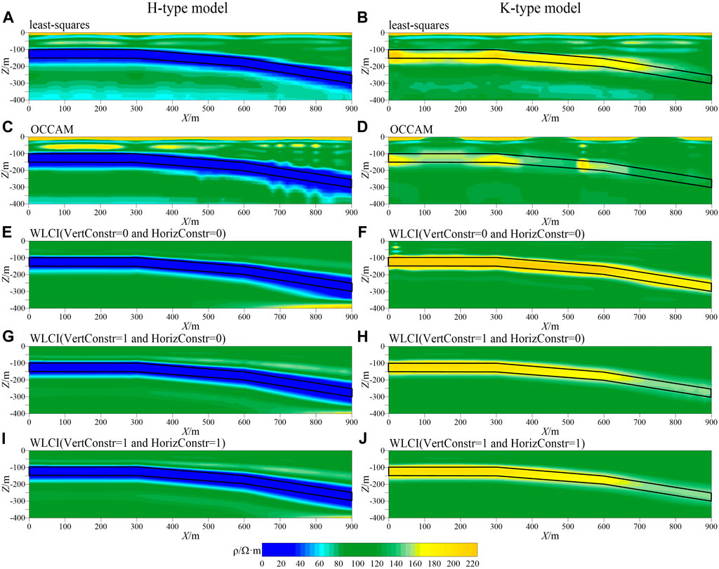
FIGURE 4. Inversion results of H-type and K-type models. (A): least-squares inversion result of H-type model. (B): least-squares inversion result of K-type model. (C): OCCAM inversion result of H-type model. (D): OCCAM inversion result of K-type model. (E): WLCI inversion result of H-type model while vertical constrained factor is 0 and horizontal constrained factor is 0. (F): WLCI inversion result of K-type model while vertical constrained factor is 0 and horizontal constrained factor is 0. (G): WLCI inversion result of H-type model while vertical constrained factor is 1 and horizontal constrained factor is 0. (H): WLCI inversion result of K-type model while vertical constrained factor is 1 and horizontal constrained factor is 0. (I): WLCI inversion result of H-type model while vertical constrained factor is 1 and horizontal constrained factor is 1. (J): WLCI inversion result of K-type model while vertical constrained factor is 1 and horizontal constrained factor is 1.

We establish multilayered models to verify the effectiveness of the inversion strategy. The models are shown in Figure 5. Two five-layer models with different layer spacings were designed. The background resistivity of the model is 100 Ω·m, the thickness of the high-resistivity layers is 20 m, the resistivity of the upper high-resistivity layer is 300 Ω·m, and the resistivity of the lower high-resistivity layer is 200 Ω·m. The resistivity in the upper high-resistivity layer from 70 to 130 m and 310–390 m along X is 50 Ω·m, and the resistivity in the lower high resistivity layer from 90 to 150 m along X is 30 Ω·m. The burial depth of the upper high-resistivity layer of model 1 is 40 m, the burial depth of the lower interface is 60 m, the burial depth of the upper interface of the lower high-resistivity layer is 120 m, and the burial depth of the lower interface is 140 m. The burial depth of the upper high-resistivity layer of model 2 is 40 m, the burial depth of the lower interface is 60 m, the burial depth of the upper interface of the lower high-resistivity layer is 100 m, and the burial depth of the lower interface is 120 m. The receiving points are located inside the rectangular transmission loop; the distance between the points is 20 m, the transmission current is 1 A, and the maximum sampling time is 10 ms. The dB/dt response data of each measuring point is obtained by forward modeling of the 1D model. In the inversion calculation, 3% Gaussian white noise is added to the dB/dt response at each time.

FIGURE 5

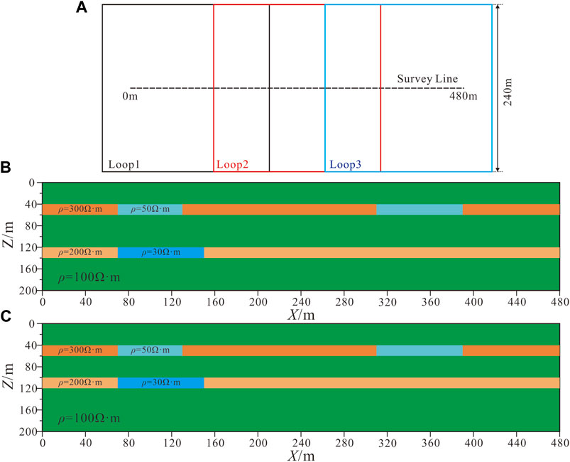
FIGURE 5. Synthetic multilayer models (various colors mean different resistivity in parts B and C). (A): Receiving and transmitting schematic. (B): Model 1 with large layer interval. (C): Model 2 with small layer interval.

Figure 6 shows the TEM decay curves at different points. A comparison of Figures 6A–C shows that at X = 40 m, the early and late time amplitudes of Model 1 and 2 are basically consistent with the uniform half space, showing the characteristics of the background strata. The middle time amplitude is small, reflecting the high resistivity. The difference between Model 1 and 2 is not evident; at X = 100 m, the early time amplitudes of Model 1 and 2 is basically consistent with that of the uniform half space, showing the characteristics of the background strata. The middle time amplitude is relatively strong, reflecting the low resistivity. Because the lower low-resistivity layer is shallower in Model 2, the low-resistivity response is more evident than that of Model 1 and appears at an earlier time. The late time response gradually increases, approaching the response of the background strata. At X = 360 m, the early and late time amplitudes of Model 1 and 2 are basically consistent with the uniform half space, showing the characteristics of the background strata. The middle time amplitude is strong, reflecting the low resistivity. There is little difference between Model 1 and 2. The single-point least-squares method, Occam method, and different horizontal and vertical constraints are used for inversion calculation. The single-point inversion results of different models and different measuring points are shown in Figure 7.

FIGURE 6

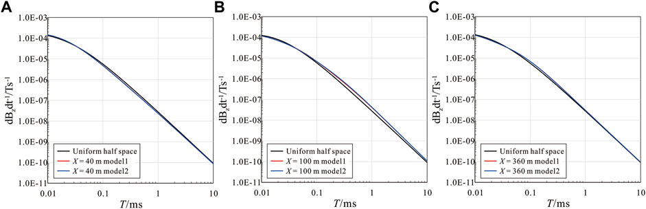
FIGURE 6. Single-point decay curves of synthetic multilayer models and corresponding uniform half space. (A): X = 40 m. (B): X = 100 m. (C): X = 360 m.

FIGURE 7

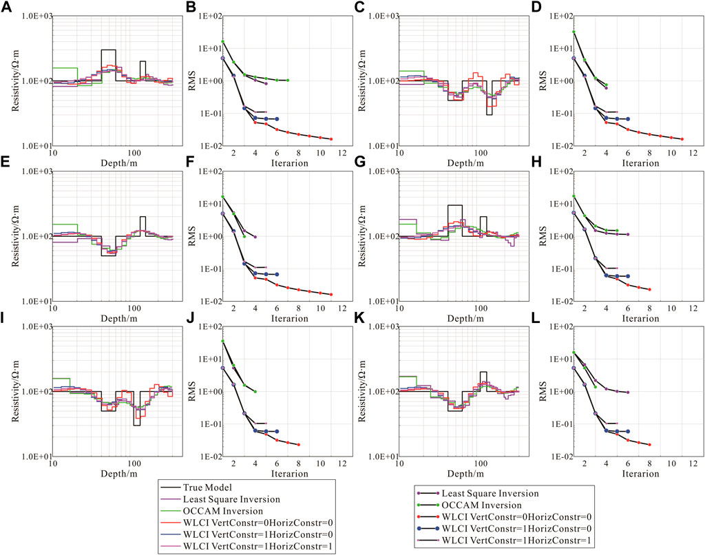
FIGURE 7. Single-point inversion results for different points. (A): Single-point inversion results at X = 40 m of model 1. (B): The Root Mean Square (RMS) at X = 40 m of Model 1. (C): Single-point inversion results at X = 100 m of model 1. (D): The RMS at X = 100 m of model 1. (E): Single-point inversion results at X = 360 m of model 1. (F): The RMS at X = 360 m of model 1. (G): Single-point inversion results at X = 40 m of model 2. (H): The RMS at X = 40 m of model 2. (I): Single-point inversion results at X = 100 m of model 2. (J): The RMS at X = 100 m of model 2. (K): Single-point inversion results at X = 360 m of model 2. (L): The RMS at X = 360 m of model 2.

The initial inversion models are all uniform half space models, and the initial resistivity of the models is 100 Ω·m while using different methods to inverse the synthetic multilayer models in Figure 7. We also use the golden section method to select the damping factor with the Occam inversion. When the layer spacing is large, all the inversion methods labeled in Figure 7 can better reflect the low-resistivity layer in the model, and the layer interface is relatively clear. When there are two high-resistivity layers (Figure 7A), the conventional 1D inversion effect is poor, and the interface of the high-resistivity layer is unclear. By reducing the layer spacing, each method can still restore the low-resistivity layer, whereas the layered interface is difficult to distinguish. The Occam method can only inverse the upper high-resistivity layer when there are two high-resistivity layers (Figure 7G). With the WLCI inversion strategy, the inversion effect of the five-layer model is good, and the low-resistivity layer interface is clear. However, after the horizontal and vertical constrained factors are applied, the inversion effect of the two high-resistivity layers is poor, and it is difficult to distinguish the lower high-resistivity layer.

A comparison of the results of different inversion methods (Figures 8A–J) shows that when the layer spacing is large, all methods better restore the low-resistivity segments in each high-resistivity layer; however, the lower high-resistivity layer inverted by the least-squares and Occam methods is transversely discontinuous. The resistivity inverted by the Occam method is smooth, but it cannot restore the lower high-resistivity layer. When the layer spacing is reduced, the continuity of the lower high-resistivity layer is poor (Occam cannot inverse the lower high-resistivity layer), and two layers of low resistivity cannot be distinguished vertically. Using the WLCI strategy, when the applied horizontal and vertical constrained factors are zero, the multilayer model can be better restored. The resistivity is more continuous in the horizontal direction, and the layer interface is clear. Increasing the constraint factor makes the resistivity more continuous in the horizontal and vertical directions. Reducing the layer spacing while increasing the constraint factors makes the inversion resistivity more continuous, but the vertical resolution decreases and cannot clearly restore the lower high-resistivity layer.

FIGURE 8

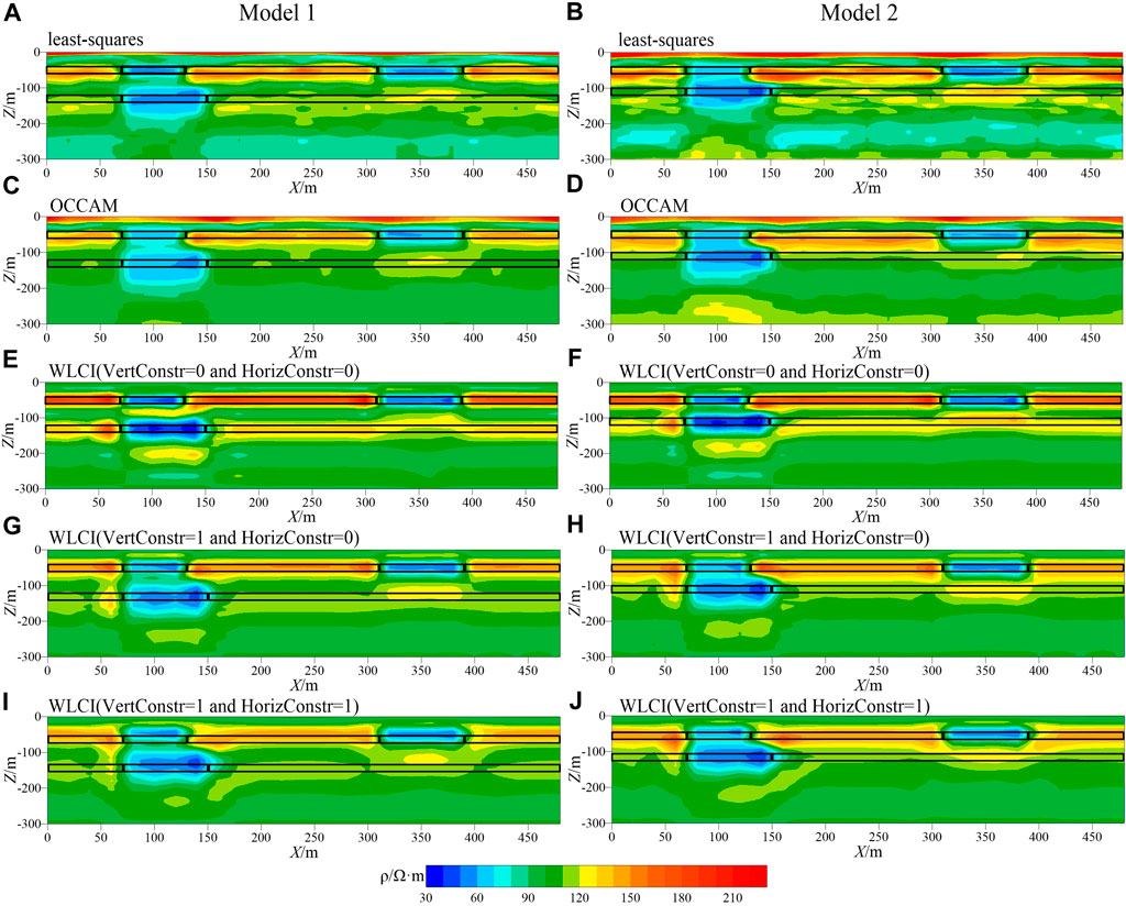
FIGURE 8. Inversion results of Model 1 and Model 2. (A): least-squares inversion result of model 1. (B): least-squares inversion result of model 2. (C): OCCAM inversion result of model 1. (D): Occam inversion result of model 2. (E): WLCI inversion result of model 1 while vertical constrained factor is 0 and horizontal constrained factor is 0. (F): WLCI inversion result of model 2 while vertical constrained factor is 0 and horizontal constrained factor is 0. (G): WLCI inversion result of model 1 while vertical constrained factor is 1 and horizontal constrained factor is 0. (H): WLCI inversion result of model 2 while vertical constrained factor is 1 and horizontal constrained factor is 0. (I): WLCI inversion result of model 1 while vertical constrained factor is 1 and horizontal constrained factor is 1. (J): WLCI inversion result of model 2 while vertical constrained factor is 1 and horizontal constrained factor is 1.

According to the synthetic model inversion results in this work, the WLCI strategy with different horizontal and vertical constrained factors is verified as effective for inversion, producing results that are laterally continuous with high vertical resolution. For sedimentary strata inversion, we must select smaller constrained factors.

4 Field data inversion

To further verify the effectiveness of the inversion strategy and the selection of weighting factors for field data inversion processing, we selected measured data collected in a region of Inner Mongolia. The data of 101 measuring points from 720 to 2,720 m of Line 35 were used for inversion calculation (Figure 9A); the distance between measuring points is 20 m. The tunnels of the #2 coal seam on the east side of the survey line have been closed and filled with mine water and soil. This is a known low-resistivity area (the range delineated by the red dotted line in Figure 9A).

FIGURE 9

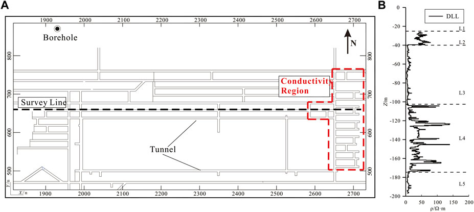
FIGURE 9. Priori information. (A): Extraction engineering diagram. (B): Borehole Dual Lateral Logging (DLL) data of resistivity.

The electrical distributions of the strata in this area are clearly shown in Figure 9B. With the exception of the shallow part above 30 m, the electrical distribution of the remaining strata from shallow to deep alternates from high-to low-resistivity in two cycles, as the L2 to L5 formations show in Figure 9Β. According to the relevant geological information, the shallow part of the strata (L1) is approximately 30 m, including the Quaternary, Neogene and Upper Cretaceous Zhidan Group. The rocks of L1 include grayish-yellow and brownish-yellow alluvial and proluvial sand and gravel with low resistivity, dark red mudstone, and sandy mudstone mixed with fine sandstone, such that the L1 formation has low resistivity. According to logging and geological data, the resistivity characteristics of formations L2 to L5 are as follows. L2: Composed of the bottom part of the Cretaceous Zhidan Group, the formations are grayish-green and light-red conglomerates characterized by high resistivity; L3: Zhiluo Formation of the Upper Jurassic strata is grayish-white and grayish-green, medium-to coarse-grained sandstone and pebbly coarse-grained sandstone mixed with siltstone and sandy mudstone presenting low resistivity; L4: The top of the Jurassic Yan’an Formation with coal seams (the #2 coal seam is located in its upper part) and nearby rock that are characterized with high resistivity; L5: The bottom of the Jurassic Yan’an Formation, with coarse sandstone and sandy mudstone and good conductivity. In summary, the strata in this area are characterized by five layers.

We use the least-squares, Occam, and WLCI methods to perform inversion calculations on the measured data. The calculation results are shown in Figure 10. The solid red lines in the figure represent the #2 coal seam. The initial model for the inversion calculation is 31 layers. The resistivity of the initial model for least-squares and Occam inversion is 30 Ω·m, and the resistivity of the initial model for WLCI inversion is 100 Ω·m. Figure 10A shows the single-point least squares inversion results, Figure 10B shows the Occam one-dimensional inversion results, and Figures 10C–E show the inversion results using different horizontal and vertical constrained factors. Figure 10 shows that the single-point least squares inversion, Occam 1D inversion, and WLCI inversion all reflect the resistivity structure of the five underground layers (L1 to L5) with good stratification that reflects the characteristics of the sedimentary strata, and the inversion of the electrical distribution characteristics is consistent with the borehole resistivity logging results. The inversion results in Figures 10A,B are basically consistent. The resistivity distribution of the Occam 1D inversion is more continuous than the least-squares inversion result, but the lower high-resistivity layer (L3) of the Occam inversion is discontinuous, and the layer interface is not clear. Figures 10C–E adopt the WLCI method, and the inversion results are basically consistent. The lateral continuity of the inversion results has been significantly improved. The lower high-resistivity layer is continuous, and the interface is clear. After increasing the constrained factor, the inversion resistivity is more continuous and smoother, but the difference between the WLCI inversion results for each layer is small. The red dotted line (2,600–2,720 m) on the east side of Figure 9B shows the characteristics of low resistivity, which is consistent with the known low-resistivity area.

FIGURE 10

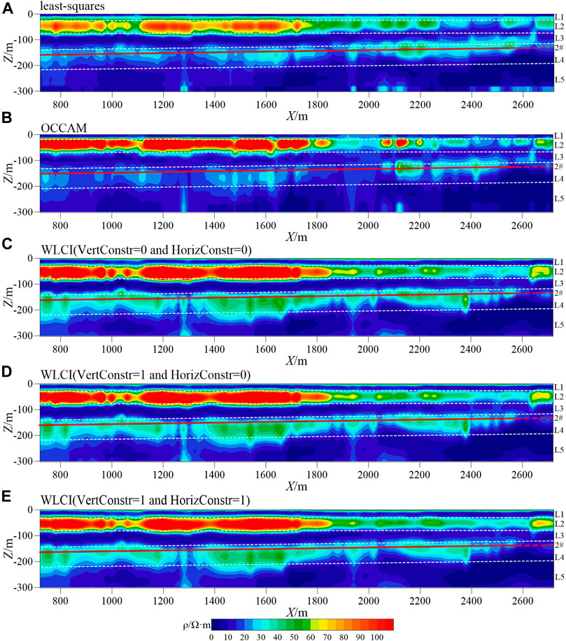
FIGURE 10. Field data inversion results. (A): least-squares inversion result. (B): Occam inversion result. (C): WLCI inversion result while vertical constrained factor is 0 and horizontal constrained factor is 0. (D): WLCI inversion result while vertical constrained factor is 1 and horizontal constrained factor is 0. (E): WLCI inversion result while vertical constrained factor is 1 and horizontal constrained factor is 1.

Therefore, for sedimentary strata, we conclude that the laterally constrained inversion strategy with different constrained factors in the horizontal and vertical directions can improve the continuity of the inversion profile and improve the vertical resolution simultaneously, making it possible to identify the layer interface. In the actual inversion, smaller constrained factors must be selected.

5 Conclusion

We successfully implemented the WLCI inversion, optimized the constrained factors, and tested it with synthetic and field data sets. Numerical experiments show that compared with the conventional 1D inversion, this new method can improve the vertical resolution by ensuring the continuity of the lateral resistivity distribution, and the inversion layer interface becomes more clear. The underground electrical structure of adjacent measuring points in the sedimentary strata is relatively continuous. Notably, the constrained factors have evident impacts on the inversion results. Small constrained factors will make the constraint less effective. On the contrary, large constrained factors may lead to serious horizontal resistivity averaging, which may eliminate real anomalies. For quasi-horizontally layered sedimentary strata, the selection of constrained factors must not be excessively large. In actual inversion, appropriate constrained factors can be determined by referring to borehole or other relevant geological data. These numerical results prove that as a quasi-2D inversion method, WLCI is effective in imaging a thin and continuous coal seam and provides a more reasonable initial model for 3D inversion.

Data availability statement

The raw data supporting the conclusion of this article will be made available by the authors, without undue reservation.

Author contributions

CS, BZ, and YL contributed to conception and design of the study. CS contributed to build the synthetic model and inversion. YL contributed to the synthetic and field data analysis. CL and GM contributed to the discussion of the results. CS wrote the first draft of the manuscript. All authors read and approved the final manuscript.

Funding

This research is funded by the National Natural Science Foundation of China (42174167, 42074120).

Acknowledgments

We thank Yang Su and Laonao Wei for their useful advice through the research.

Conflict of interest

The authors declare that the research was conducted in the absence of any commercial or financial relationships that could be construed as a potential conflict of interest.

Publisher’s note

All claims expressed in this article are solely those of the authors and do not necessarily represent those of their affiliated organizations, or those of the publisher, the editors and the reviewers. Any product that may be evaluated in this article, or claim that may be made by its manufacturer, is not guaranteed or endorsed by the publisher.

References

Auken, E., Christiansen, A. V., Jacobsen, L. H., and Sørensen, K. I. (2008). A resolution study of buried valleys using laterally constrained inversion of TEM data. J. Appl. Geophys. 65 (1), 10–20. doi:10.1016/j.jappgeo.2008.03.003

CrossRef Full Text | Google Scholar

Auken, E., and Christiansen, A. V. (2004). Layered and laterally constrained 2D inversion of resistivity data. Geophysics 69 (3), 752–761. doi:10.1190/1.1759461

CrossRef Full Text | Google Scholar

Auken, E., Thomsen, P., and Sorensen, K. (2000). “Lateral constrained inversion (LCI) of profile-oriented data—the resistivity case,” in Proceedings of the 6th EAGE/EEGS Meeting, Bochum, Germany, September 2000, EL06.

Google Scholar

Cai, J., Qi, Y., and Yin, C. (2014). Weighted laterally-constrained inversion of frequency-domain airborne EM data. Chin. J. Geophys. 57 (3), 953–960.

Google Scholar

Christensen, N. B., Reid, J. E., and Halkjær, M. (2009). Fast, laterally smooth inversion of airborne time-domain electromagnetic data. Near Surf. Geophys 7 (5–6), 599–612. doi:10.3997/1873-0604.2009047

CrossRef Full Text | Google Scholar

Constable, S. C., Parker, R. L., and Constable, C. G. (1987). Occam's inversion; a practical algorithm for generating smooth models from electromagnetic sounding data. Geophysics 52 (3), 289–300. doi:10.1190/1.1442303

CrossRef Full Text | Google Scholar

Danielsen, J. E., Auken, E., Jørgensen, F., Søndergaard, V., and Sørensen, K. I. (2003). The application of the transient electromagnetic method in hydrogeophysical surveys. J. Appl. Geophys. 53, 181–198. doi:10.1016/j.jappgeo.2003.08.004

CrossRef Full Text | Google Scholar

Farquharson, C., and Oldenburg, D. (1993). Inversion of time-domain electromagnetic data for a horizontally layered Earth. Geophys. J. Int. 114, 433–442. doi:10.1111/j.1365-246x.1993.tb06977.x

CrossRef Full Text | Google Scholar

Fitterman, D. V., and Stewart, M. T. (1986). Transient electromagnetic sounding for groundwater. Geophysics 51, 995–1005. doi:10.1190/1.1442158

CrossRef Full Text | Google Scholar

Fountain, D., Smith, R., Payne, T., and Limieux, J. (2005). A helicopter time domain EM system applied to mineral exploration: System and data, 23. doi:10.3997/1365-2397.23.1089.26741First Break

CrossRef Full Text

Guptasarma, D. (1982). Computation of the time-domain response of a polarizable ground. Geophysics 47 (11), 1574–1576. doi:10.1190/1.1441307

CrossRef Full Text | Google Scholar

Haber, E., and Schwarzbach, C. (2014). Parallel inversion of large-scale airborne time-domain electromagnetic data with multiple OcTree meshes. Inverse Probl. 30 (5), 55011. doi:10.1088/0266-5611/30/5/055011

CrossRef Full Text | Google Scholar

Huang, H., and Palacky, G. J. (2010). Damped least-squares inversion of time-domain airborne EM data based on singular value decomposition. Geophys. Prospect. 39 (6), 827–844. doi:10.1111/j.1365-2478.1991.tb00346.x

CrossRef Full Text | Google Scholar

Hui, Z., Liu, Y., Yin, C., Su, Y., Ren, X., Zhang, B., et al. (2021). Detection of coal spontaneous combustion using the TEM method: A synthetic study. Pure Appl. Geophys. 178 (4), 3987–4000. doi:10.1007/s00024-021-02829-5

CrossRef Full Text | Google Scholar

Jiang, Z., Liu, L., Liu, S., and Yue, J. (2019). Surface-to-underground transient electromagnetic detection of water-bearing goaves. IEEE Trans. Geosci. Remote Sens. 57 (8), 5303–5318. doi:10.1109/tgrs.2019.2898904

CrossRef Full Text | Google Scholar

Johansen, H. K., and Sorensen, K. (1979). Quasi fast Hankel transform. Geophys. Prospect. 27, 876–901. doi:10.1111/j.1365-2478.1979.tb01005.x

CrossRef Full Text | Google Scholar

Liu, Y., Yin, C., Qiu, C., Hui, Z., Zhang, B., Ren, X., et al. (2019). 3D inversion of transient EM data with topography using unstructured tetrahedral grids. Geophys. J. Int. 217 (1), 301–318. doi:10.1093/gji/ggz014

CrossRef Full Text | Google Scholar

Lu, J., Lei, D., and Ren, H. (2022). Laterally constrained inversion of airborne transient electromagnetic data with induced-polarization effects. Prog. Geophys. (in Chinese) 37 (1), 0220–0229. doi:10.6038/pg2022FF0045

CrossRef Full Text | Google Scholar

Nabighian, M. N. (1979). Quasi-static transient response of a conducting half-space - an approximate representation. Geophysics 44, 1700–1705. doi:10.1190/1.1440931

CrossRef Full Text | Google Scholar

Ren, X. Y., Yin, C. C., Macnae, J., Liu, Y. H., and Zhang, B. (2018). 3D time-domain airborne electromagnetic inversion based on secondary field finite-volume method. Geophysics 83, E219–E228. doi:10.1190/geo2017-0585.1

CrossRef Full Text | Google Scholar

Santos, F. A. M. (2004). 1-D laterally constrained inversion of EM34 profiling data. J. Appl. Geophys. 56 (2), 123–134. doi:10.1016/j.jappgeo.2004.04.005

CrossRef Full Text | Google Scholar

Si, Y., Li, M., Liu, Y., and Guo, W. (2020). One-dimensional constrained inversion study of TEM and application in coal goafs' detection. Open Geosci 12 (1), 1533–1540. doi:10.1515/geo-2020-0148

CrossRef Full Text | Google Scholar

Siemon, B., Auken, E., and Christiansen, A. V. (2009). Laterally constrained inversion of helicopter-borne frequency-domain electromagnetic data. J. Appl. Geophys. 67 (3), 259–268. doi:10.1016/j.jappgeo.2007.11.003

CrossRef Full Text | Google Scholar

Stacey, W. M. (1976). “Transient electromagnetic fields,” in Section 1.2: Field equations and boundary conditions (Berlin, Germany: Springer-Verlag), 5–6.

Google Scholar

Yang, D., and Oldenburg, D. W. (2012). Three-dimensional inversion of airborne time-domain electromagnetic data with applications to a porphyry deposit. Geophysics 77, B23–B34. doi:10.1190/geo2011-0194.1

CrossRef Full Text | Google Scholar

Yang, H., Li, F., Yue, J., Liu, X., Zhao, H., Zhan, J., et al. (2016). Molecular cloning, expression, and functional analysis of the copper amine oxidase gene in the endophytic fungus Shiraia sp. Slf14 from Huperzia serrata. J. China Univ. Mining Technol. 45 (6), 8–13. doi:10.1016/j.pep.2016.07.013

PubMed Abstract | CrossRef Full Text | Google Scholar

Yin, C., Qiu, C., Liu, Y., and Cai, J. (2016). Weighted laterally-constrained inversion of time-domain airborne electromagnetic data. J. Jilin Univ. (Earth Sci. Ed.) 46 (1), 254–261.

Google Scholar

Zhang, B., Engebretsen, K. W., Fiandaca, G., Cai, H., and Auken, E. (2021). 3D inversion of time-domain electromagnetic data using finite elements and a triple mesh formulation. Geophysics 86 (3), E257–E267. doi:10.1190/geo2020-0079.1

CrossRef Full Text | Google Scholar

Zhang, J., Zhou, G., Liu, Z., Sun, N., Zhang, F., and Wang, Z. (2022). Lateral constrained inversion of E-Ex wide field data. J. China Coal Soc. 47 (7), 2698–2707.

Google Scholar