The application of Monte Carlo modelling to quantify in situ hydrogen and associated element production in the deep subsurface

1 Introduction

Due to advances in technology, computational-based approaches have now become the norm in modelling natural systems (e.g., Crutchfield, 1994; Shalizi, and Crutchfield, 2001; Hopper and Rice, 2008). In particular, increases in computational capabilities allow refinement of new and existing models and datasets to progressively generate more sophisticated numerical models in a diverse range of fields, such as physics, geology, ecology, and epidemiology to provide additional insight into a wide range of natural systems globally (e.g., Wilensky and Rand, 2015; Gillman and Gillman, 2019). Such predictive models are essential to evaluate complex datasets involving multiple inputs. They are essential in particular for integrating data generated in disparate locations/geologic settings and to extrapolate to regional-global processes occurring on Earth and beyond (e.g., other planets and moons). One way to do this integrates large global datasets is to implement a Monte Carlo based approach (Gallagher et al., 2009). Broadly speaking, this technique allows for a value to be taken from a defined range based on a defined probability. This number can then be used within a deterministic calculation to generate a single model outcome. This process is then repeated until the rolling averages of key outputs of the model stabilize and do not change significantly with additional output data (i.e., the model converges) (Benedetti et al., 2011). At this point, analysis of the output data provides a way to statistically evaluate the most probable outcome(s) of the model based on each of the input parameters, as well as to demonstrate the sensitivity of input parameters (i.e., how a range in each input can impact variables derived from each calculation).

Due to the benefits of this approach, the earth sciences and geochemistry community has been incorporating this technique in a variety of applications (e.g., Sambridge and Mosegaard, 2002; Gallagher et al., 2009; Warr et al., 2015; Liu and Liang, 2017; Sakan et al., 2019; Wang et al., 2020; Karolytė et al., 2022). One powerful application which remains underexplored is the in situ production of key elements and compounds of biogeochemical and/or economic interest generated through the natural decay of U, Th, and K within a wide range of crustal settings. For example, recent papers re-evaluated the mechanisms generating crustal noble gases in the deep crust (Lippmann-Pipke et al., 2011; Holland et al., 2013; Warr et al., 2018; Warr et al., 2022), and proposed novel habitability models in the deep Earth and marine sediments based on hydrogen generation via radiolytic decomposition of water (e.g., D’Hondt et al., 2009; Sherwood Lollar et al., 2014; Sherwood Lollar et al., 2021; Li et al., 2016; Sauvage et al., 2021). Documenting, quantifying, and refining these radiogenic and radiolytic processes with respect to their ability to potentially generate H₂, ⁴He, ⁴⁰Ar, SO₄^2-, N₂, organic molecules and others within crustal settings on Earth and beyond has considerable recent interest with respect to the understanding of early Earth processes and prebiotic chemistry, constraining habitability models on Earth and beyond, and the formation of economic resources (e.g., ⁴He) over geologic timescales (e.g., Lin et al., 2005a; Lin et al., 2005b; Onstott et al., 2006; Blair et al., 2007; Lefticariu et al., 2010; Sherwood Lollar et al., 2014; Dzaugis et al., 2016; Li et al., 2016; Bouquet et al., 2017; Altair et al., 2018; Dzaugis et al., 2018; Tarnas et al., 2018; 2021; Yi et al., 2018; National Academies of Sciences, Engineering, and Medicine, 2019; Warr et al., 2019; Adam et al., 2021; Boreham et al., 2021; Warr et al., 2021b; Li et al., 2021; Sauvage et al., 2021; Vandenborre et al., 2021; Li et al., 2022; Warr et al., 2022; Nisson et al., 2023).

Critical to advancing understanding of these topics to the next level is quantitative evaluation of the degree to which local variability/uncertainty in the key variables (e.g., porosity, radioelement concentration, and sulfide mineral distribution) control production of these molecules in subsurface settings. Some of the most common methods which are typically applied in order to address this include using average values, or less commonly, ranges covering minimum or maximum values. Uncertainties are often unaddressed. Identifying, constraining and combining these estimated co-dependent values and associated uncertainties to generate more accurate production rates and ranges remains a challenge.

This study applies a novel Monte Carlo approach, building on previous methodology, to address this critical issue and to introduce a quantifiable measure of most probable production estimate for the types of investigations outlined above. Previous approaches have taken single values for input parameters such as averages (e.g., mean or median values) often without considering uncertainty, or a range of probable input parameters by site/region (i.e., the extreme upper and lower estimates) (to incorporate the key variables into radiolytic models (Lin et al., 2005a; Lin et al., 2005b; Onstott et al., 2006; Dzaugis et al., 2016; Dzaugis et al., 2018; Warr et al., 2019; Sauvage et al., 2021; Li et al., 2022). Taking this approach has the benefit of placing absolute constraints on magnitudes of processes (Holland and Gilfillan, 2013; Li et al., 2016; Tarnas et al., 2021). However, as a consequence, values generated represent the extreme outputs (i.e., the maximum and minimum estimates) with no insight into the most probable estimate. Likewise, it does not consider the relative and cumulative effects of inherent natural variation present for each input parameter. As a consequence, while this method provides essential constraints on the absolute magnitude, this approach fails to provide either an accurate assessment of the most reasonable in situ production rate or a probabilistic production range for any system.

Here we demonstrate a novel way to consider and incorporate the effects of natural variability on subsurface radiolytic models for the first time by integrating a Monte Carlo technique to recent radiolytic/radiogenic models (Lin et al., 2005b; Li et al., 2016; Tarnas et al., 2018; 2021; Li et al., 2022). Specifically, we apply a Monte Carlo approach to data from the suite of papers published on the Kidd Creek Observatory in Canada where production of H₂, ⁴He, ⁴⁰Ar, SO₄^2- has been estimated using the methods outlined previously (Sherwood Lollar et al., 2014; Li et al., 2016; Warr et al., 2019). Focusing on this well-studied site allows direct comparison between the Monte Carlo models outlined here and previous production estimates to highlight the key advances represented by this approach. Specifically, the novel Monte Carlo-based modelling technique demonstrates how the natural variability associated with each parameter can be simultaneously considered to generate next-generation models capable of evaluating the range and probability of in situ production in a natural setting and, by extension, providing a foundation for extrapolating production rates based on locally generated data to regional/global estimates.

2 Geologic setting

Kidd Creek Observatory established in 2008, is located approximately 24 km north of the town of Timmins, Ontario, (Canada). The saline fracture fluids continuously discharging have been monitored for geochemical, isotopic and microbiological parameters for almost 15 years to date, and represent, to our knowledge, the longest time series investigation of subsurface fluids available for the scientific community at such a profound depth (2.4 km below surface). The observatory itself is situated within an active mine extracting copper, zinc and silver from a 2.7 Ga age stratiform Volcanogenic Massive Sulfide (VMS) deposit located within the Kidd-Munro assemblage of the Southern Volcanic Zone of the Abitibi greenstone belt of the Superior Province of the Canadian Shield (Bleeker and Parrish, 1996; Thurston et al., 2008).

The Kidd-Munro assemblage where the observatory is located consists of a series of steeply dipping interlayered ultramafic, mafic, felsic, and metasedimentary deposits and is an Archean aged hydrothermal vent system. The stringer ore, which represents one of the primary economic resources being extracted in the mine, formed as a result of silica and metal-rich hydrothermal fluid circulation below the seafloor and is chiefly associated with the upper felsic region. Overlying the stringer ore region are banded and massive sulfide ores which are commonly considered to have been initially deposited as inorganic precipitates which were generated when hydrothermal solutions rich in metals interacted with the seawater. Within the Kidd-Munro assemblage are intermittent argillite to chert carbonaceous horizons where are considered to represent the accumulation of proximal seafloor sediments during periods of volcanic quiescence. During this stage this Precambrian hydrothermal seafloor setting underwent extensive carbonization associated with CO₂-rich hydrothermal fluids resulting in carbonate formation in less reduced zones and graphitic deposits in more reducing zones (Ventura et al., 2007). Subsequent to deposition, the last major regional metamorphic event at 2.67–2.69 Ga metamorphosed the Kidd-Munro assemblage to greenschist facies with the last identified metasomatic episode occurring at 2.64 Ga after which the region is considered tectonically quiescent (Davis et al., 1994; Bleeker and Parrish, 1996; Thurston et al., 2008; Berger et al., 2011; Li et al., 2016). During this ongoing period of quiescence, the study of Flowers et al. (2006) estimated that this craton has been highly stable with low erosion rates of ≤2.5 m/million years.

3 Materials and methods

3.1 Existing model overview

The model presented here is a Monte Carlo adaptation of previous quantitative numerical approaches which are outlined in this section for modelling radiolytically-derived products in the subsurface (Lin et al., 2005a; Lin et al., 2005b; Li et al., 2016; Tarnas et al., 2018; Warr et al., 2019; Tarnas et al., 2021). Annual ⁴He and ⁴⁰Ar production rates (moles/m³ per year) were calculated by incorporating U, Th, and K concentrations into the equations of Ballentine and Burnard (2002):

${}^{4}He=\frac{\left[\left(3.115\times {10}^6+1.272\times {10}^5\right)U+\left(7.710\times {10}^5\right)Th\right]}{N_A}\times {\rho }_{bulk}\times {10}^6(1)$

${}^{40}Ar=\frac{102.2\times K}{N_A}\times {\rho }_{bulk}\times {10}^6(2)$

where U, Th, and K represent concentrations of uranium, thorium and potassium (ppm), ρ_bulk represents density of the system in g/cm³ and N_A is Avogadro’s number. ρ_bulk is a function of the density of the rock, density of the fluid, and their relative proportions. This term ensures production is scaled and standardized to 1 m³ of system volume incorporating the effects of porosity (as opposed to previous studies which only applied the density of the rock itself (ρ_r)), here to specifically consider elemental production per m³ of rock (e.g., Tarnas et al., 2018; Warr et al., 2019; Tarnas et al., 2021). This adaptation is relatively minor as applying ρ_bulk as opposed to ρ_r typically results in a relatively small difference (≤5%) in the density term when porosity is low (≤8%). All systems considered in this study are of very low porosity (typically < 1–2%). ρ_bulk is calculated via Eq. 3:

${\rho }_{bulk}=\mathit{\Phi }\times {\rho }_w+\left(1-\mathit{\Phi }\right)\times {\rho }_r(3)$

where Φ represents porosity (0-1) and ρ_w and ρ_r represents the density of fluid and host rock respectively in g/cm³.

To calculate the theoretical H₂ production rates attributed to radioactive decay alone at each location, the same approach as Sherwood Lollar et al. (2014), and Tarnas et al. (2018) was used. Briefly, this approach calculates the total H₂ yield (Y_H2) in moles/m³ rock per year using the following equations:

$Y_{H2}=\left[\sum \left(\frac{E_{net,i}\times \left(G_{H2i}/100\right)}{N_A}\right)\right]{\times \rho }_{bulk}\times {10}^3(4)$

where i designates the radiation type (α, β, or γ) G_H2 is the number of H₂ molecules produced per 100 eV of radiation and E_net is the net dosage absorbed by the water from the specified radiation type (eV/kg per year). Values of 1.32, and 0.25 were used for G_H2α and G_H2γ from Sauvage et al. (2021) and a value of 0.6 for G_H2β was taken from Lin et al. (2005a) and references therein. To calculate E_net the following calculation is used:

$E_{net,i}=\sum \left[\frac{E_{Xi}\times 6.241509\times {10}^{15}\times W\times S_i}{\left(1+W\times S_i\right)}\right](5)$

where X represents the radioelement (U, Th, K), E is the apparent dosage from radioactive element decay (Gy/Ka), 6.241509 ×10¹⁵ is the conversion factor from Gy (j/kg) per ka to eV/kg per year, W is the unitless weight ratio of pore water to rock, and S is the stopping power of minerals with respect to the radiation type (i). The S_α, S_β, S_γ values used here are 1.5, 1.25 and 1.14 respectively and E values of 0 (E_Kα), 0.782 (E_Kβ), 0.243 (E_Kγ), 0.061 (E_Thα), 0.027 (E_THβ), 0.048 (E_THγ), 0.218 (E_Uα), 0.146 (E_Uβ), 0.113 (E_Uγ) which correspond to 1ppm U, 1 ppm Th, and 1 wt% K, the latter values following Lin et al. (2005b), Lin et al. (2005a), Tarnas et al. (2018), Tarnas et al. (2021), and Warr et al. (2019). W is calculated via the following equation:

$W=\frac{\mathrm{\Phi }\times {\rho }_w}{\left(1-\mathit{\Phi }\right)\times {\rho }_r}(6)$

Using Eqs 4, 5, the H₂ yield is calculated and, by combining with the calculated ⁴He and ⁴⁰Ar production rates, the theoretical H₂/⁴He and H₂/⁴⁰Ar unitless production ratios from radioelement decay can be calculated for a given porosity (Lin et al., 2005a; Sherwood Lollar et al., 2014; Warr et al., 2019).

To calculate the theoretical SO₄^2- production rates, the equations of Li et al. (2016) and Tarnas et al. (2021) were used. This approach calculates the production rate of dissolved SO₄^2- in moles per liter per year (C_SO4) using the following equations:

$C_{SO4}=\frac{Y_{SO4}\times \left(C_{sulfide}/100\right)\times S_{Sulfide}\times {\rho }_w}{W}(7)$

$Y_{SO4}=\sum E_{net,i}\times G_{SO4i}(8)$

where Y_SO4 is the yield of sulfate (moles per m² of sulfide surface area), C_sulfide is the concentration of sulfides in the rock matrix (in %), S_sulfide is the average surface area of sulfides in the rock matrix (m² sulfide per kg), and G_SO4 represents the moles of SO₄ which is produced per m² of sulfide as a function of dose. To convert C_SO4 to production in moles per bulk m³ of rock per year (P_SO4) Eq. 9 is applied:

$P_{SO4}=C_{SO4}\times 1000\times \mathit{\Phi }(9)$

where 1000 represents the number of liters in 1 m³ which is scaled here to the porosity.

3.2 Incorporating a Monte Carlo approach

As demonstrated in Section 3.1, all production rates depend on a minimum of three intersecting variables (⁴⁰Ar) up to a maximum of eight (SO₄^2-) with some variables being factored in multiple times (e.g., porosity and fluid and rock density). As a consequence, incorporating a Monte Carlo method allows this non-linear complexity to be readily incorporated. This is implemented here using Kidd Creek where a Monte Carlo based approach can be readily applied and evaluated against previous production estimates that all used similar input parameters (Holland et al., 2013; Sherwood Lollar et al., 2014; Li et al., 2016; 2021; Warr et al., 2018; Lollar et al., 2019; Warr et al., 2019; Warr et al., 2021a; Sherwood Lollar et al., 2021). From Eqs 1–9 the following eight key parameterized variables were identified and are summarized in Table 1: 1. Porosity, 2. Density of fluid, 3. Density of rock, 4-6. Concentrations of radioelements (U, Th, K), 7. Sulfide concentration, and 8. Sulfide surface area. Prior to this study most studies have either used a single value from the literature (typically a reported average), or maxima and minima values to generate upper and lower production rates of H₂, ⁴He, ⁴⁰Ar, SO₄^2- (Lin et al., 2005a; Lin et al., 2005b; Li et al., 2016; Tarnas et al., 2018; 2021; Warr et al., 2019). See references in these papers for specific sources of the values used.

TABLE 1

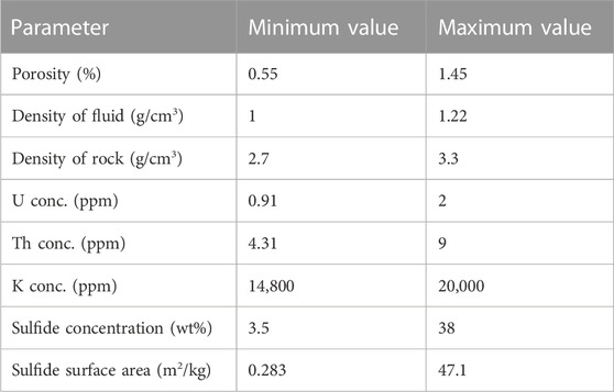
TABLE 1. Range of values for Kidd Creek Observatory used in this Monte Carlo-based approach based on published values, as described in full in the main text.

In the case of Kidd Creek Observatory, previous ranges used for each parameter are presented in Table 1. For porosity, a range of 0.55%–1.45% was selected, based on the 1% ±0.45 range used previously in noble gas studies at the site (Holland et al., 2013; Warr et al., 2018). This range is consistent with measured and modelled porosity estimates in fractured rock settings which range from 0.1% to 2.3%, and have an average porosity of 1.0% ±0.45% (Stober, 1997; Guillot et al., 2000; Aquilina et al., 2004; Stober and Bucher, 2007; Bucher and Stober, 2010; Stober, 2011; Holland et al., 2013). This range is also consistent with the range used by Sherwood Lollar et al. (2014) to factor in a porosity as a function of depth in crystalline rock settings adapted from the depth-porosity model of Bethke (1985) and outlined in Eq. 10:

$\mathit{\Phi }=\frac{{1.6}^{\left(-z/4.8\right)}}{100}(10)$

where ϕ is bulk porosity (%) and z is depth (km). For the upper 10 km, this approach similarly predicts an average bulk porosity of 0.96% with a relative uncertainty of 0.45%. To date all of these approaches are consistent and provide a relatively well constrained range for porosity for the Precambrian Shield fractured rocks of 0.55%–1.45%. It is worth noting however that as explained in the previous studies, this parameter typically introduces the largest uncertainty in the calculated outputs (e.g., Warr et al., 2018).

A range of 1–1.22 g/cm³ was used for fluid density to reflect the maximum potential spectrum of fluids ranging from freshwater to the highly saline fracture fluids measured at the site containing up to 220 g/L based on the geochemical data presented in Lollar et al. (2019) and Warr et al. (2021a). Meanwhile, a range of 2.7–3.3 g/cm³ was applied for rock density which incorporates the range of densities associated with crustal settings containing mafic-ultramafic, felsic and meta-sedimentary lithologies as is the case for Kidd Creek (e.g., Sherwood Lollar et al., 1993; Bleeker and Parrish, 1996; Thurston et al., 2008) and for comparable crystalline settings globally (Lippmann et al., 2003; Holland et al., 2013; Sherwood Lollar et al., 2014; Heard et al., 2018). For U, Th, and K concentrations, ranges of 0.91–2.00, 4.31–9.00, and 14,800–20000 ppm (1.48%–2%), respectively, were chosen following Li et al. (2016) which selected this as a representative range for these elements for the Abitibi Sub province based on Ketchum et al. (2008); Moulton et al. (2011). Values from within this range were those used previously in noble gas and hydrogen production-based studies (Holland et al., 2013; Warr et al., 2018; Warr et al., 2019) which allows direct comparison between the model presented here and these previous studies.

With respect to sulfide (pyrite) concentrations, these were based on the study of Li et al. (2016) which estimated pyrite concentrations of 3.5% in the non-ore zone and 38% pyrite in the massive sulfide ore zone based on mass balance calculations from published elemental inventory data (Hannington et al., 1999). In this study, as with the previous study by Li et al. (2016), pyrite was the only sulfide considered here as the production of sulfate as a function of indirect radiolysis has previously been experimentally investigated (Lefticariu et al., 2010) and in at Kidd Creek it represents the dominant sulfide mineral present (∼70% of total sulfide) based on the study by Hannington et al. (1999). Lastly, with respect to sulfide surface area, a range of 0.283–47.1 m²/kg was considered here. This range incorporates the surface area as modelled by Li et al. (22.6 m²/kg) and expands this to consider a grain size range of 1 cm–60 μm following the sphere packing model of Altair et al. (2018) in order to reasonably consider the natural variability of pyrite grains in both ore-rich and ore-poor regions of Kidd Creek.

To incorporate the Monte Carlo based approach, two types of Monte Carlo methods were applied. In the Random Distribution Model (RDM), a value was selected at random for each variable from within the maximum and minimum ranges outlined in Table 1 to generate a set of feasible system parameters. These were then incorporated into Eqs 1–9 and the resultant in situ production of ⁴He, ⁴⁰Ar, H₂ and SO₄^2- were calculated. This process was then repeated a total of 1,000,000 times using different randomly selected values to calculate the resulting spectrum of uniformly distributed potential production values for ⁴He, ⁴⁰Ar, H₂, and SO₄^2-. In the second model, the Standard Distribution Model (SDM), a standard distribution approach was applied. Specifically, numbers were generated with a normal (standard) distribution using the mid-point value of each range. Using this approach, the central values within the range are more probable and values which approach the upper and lower limits are progressively less likely to be selected. To assign the standard deviation, the difference between this midpoint and the upper value was calculated and divided by three (i.e., the upper and lower limit represented 3σ from the mean). 3σ was selected here so 99.7% of all numbers generated through this approach would lie within the specified ranges and to ensure all generated values (including outliers) for variables close to zero (e.g., porosity, U concentration), would remain greater than zero. The exception to this is pyrite abundance and sulfide surface area, as highlighted by Table 1, which both vary considerably as a function of the proximity to the ore body, with abundances ranging between 3.5% and 38% and surface areas scaling from 0.283 to 47.1 m²/kg where surface area rapidly increases as grain size decreases. Here, given the large difference between the mid-point and the upper and lower ranges, a 5σ approach was applied to ensure only positive values were returned using this approach.

4 Results

4.1 Production rates

The maximum, minimum, average, and standard deviation for the annual production of each element per bulk cubic meter of rock is provided in Table 2 for each model and plotted in Figure 1.

TABLE 2

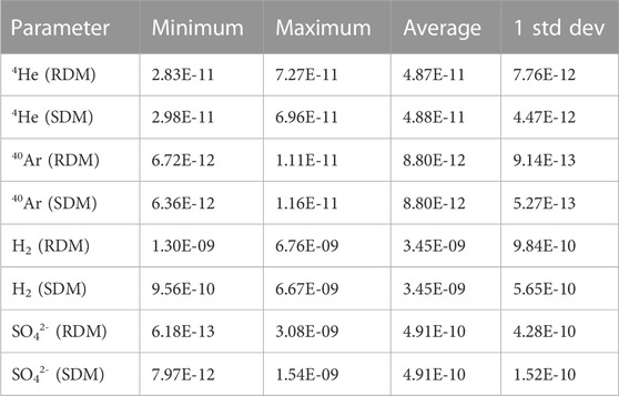
TABLE 2. Production rates for ⁴He, ⁴⁰Ar, H₂, and SO₄^2- per bulk m³ of rock per year determined using Eqs 1–9, coupled with the two Monte Carlo modelling approaches incorporating the input parameters provided in Table 1 and described in full in the main text. Each value represents the result of one million generated values via the two Monte Carlo models RDM and SDM. All production rates are in moles per bulk m³ per year.

FIGURE 1

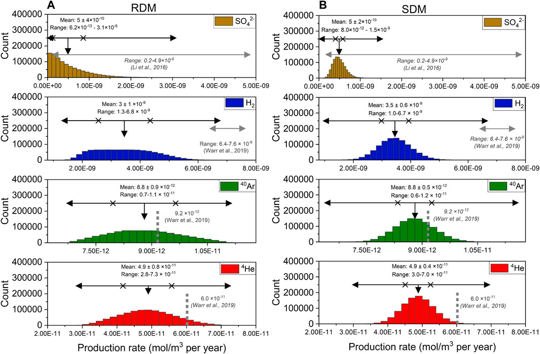
FIGURE 1. Production rates for ⁴He, ⁴⁰Ar, H₂, and SO₄^2- in moles per bulk m³ rock per year determined using Eqs 1–9, via the random distribution Monte Carlo approach (RDM) (A) and the standard distribution Monte Carlo approach (SDM) (B). The results incorporate the input parameters provided in Table 1 and are described in full in the main text. Previously calculated production rates by Li et al. (2016) for SO₄^2-; Warr et al. (2019) for H₂, ⁴He, and ⁴⁰Ar are plotted as light grey horizontal lines for H₂ and SO₄^2- and in grey vertical hatched lines for ⁴He and ⁴⁰Ar. SO₄^2- production from Li et al. (2016) is converted from the reported production (moles per liter per year) to production in moles per m³ bulk rock per year using Eq. 9 and a porosity of 1% as in the Li et al. (2016) published model. On all figures the black horizontal arrows represent the range (maximum-minimum) for the results from this study, the vertical black arrows represent the average (mean), and the crosses represent the associated standard deviation (1 σ).

Table 2 and Figure 1 show that for all four products the same average (mean) values (within uncertainty) result from both the RDM and SDM Monte Carlo approaches. Likewise, the absolute (minimum-maximum) range is comparable between the models. The most significant difference between the two model approaches is the consistently larger standard deviation of the mean (Table 2) for the RDM versus the SDM.

4.2 Model robustness

A convergence-based evaluation was applied to evaluate the robustness of the Monte Carlo model outputs based on the method applied by Benedetti et al. (2011). For this, an additional 10 discrete datasets were generated for each model for the Kidd Creek Observatory using the same input parameters, but this time each consisting of 100,000 outputs instead of the previous one million. Each of these datasets therefore are an order of magnitude smaller than the dataset used to generate the values presented in Table 2 and Figure 1. In this case, for each of the discrete datasets, the minimum, maximum, average, and standard deviations were determined as per the overall dataset in Table 2. These values were then individually collated from the 10 datasets, and from these 10 values, an average and standard deviation were determined. Lastly, the relative standard deviation was determined by calculating the variability, here considered the absolute standard deviation as a percentage of the average values. This approach allows evaluation of the convergence for each of the values presented in Table 2 as a function of sample size. This study considers convergence has been reached for a given parameter when the calculated variability is within 1% following Benedetti et al. (2011). Results are given in Table 3.

TABLE 3

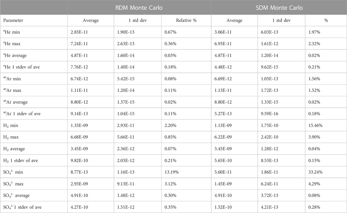
TABLE 3. Average, standard deviation, and relative percentage of each statistic presented in Table 2 (min, max, average, standard deviation) for each element. These were determined by generating an additional 10 discrete data sets of 100,000 values using the same approach as outlined in the main text. For each data set of 100,000 the min, max, average and standard deviation was then calculated as with those presented in Table 2 for the full data set. These were then compiled from the 10 data sets and an average and standard deviation was calculated for each of these outputs. Additionally, the relative percentage the standard deviation represents with respect to the mean is presented to show variability. All production rates are in moles per bulk m³ rock per year.

Table 3 demonstrates that convergence is reached for all elements for the average production rate and the associated standard deviation in both models by 100,000 data with less than 0.4% variance at 1 sigma in all cases. Consequently, both Monte Carlo techniques presented here can produce robust and reproducible average production rates and an associated standard deviation from a generated dataset an entire order of magnitude lower than the sample size which was generated and analyzed in Table 2. This therefore demonstrates the robustness of the model at generating a most probable production rate and associated uncertainty even at relatively small sample sizes (100,000 data). This not only highlights that this approach is not only capable of numerically defining the range of possible values but also providing critical statistical insight into the probability of the production estimates for a natural setting.

With respect to the generated minimum and maximum values and the production range this represents, Table 3 demonstrates that there is more associated relative variability at the 100,000-output level, particularly with the SDM Monte Carlo approach. This is expected as these ‘extreme’ values depend on a combination of multiple uppermost and/or lowermost inputs which probabilistically have a lower chance of co-occurring and so are not as frequent, especially when a normal distribution is applied. This likewise highlights why the standard deviations are considerably lower for the SDM Monte Carlo approach as highlighted in Section 3.1. Continuing to focus on variability though, the greatest relative variability is present for the lowest estimated production rates for both H₂ and SO₄^2-. These two species (H₂ and SO₄^2-) depend on the greatest number of input variables and so, from a probabilistic standpoint, this makes sense, as in order to generate production rates for these two species requires the greatest co-occurrence of max/min values to be selected from the input ranges.

The magnitude of relative uncertainty in Table 3 is also intrinsically a function of the scale involved. The same absolute variability around a smaller value will always translate to a higher relative variability. When the absolute variability (standard deviation) in Table 3 is considered, this is actually consistently and considerably lower compared to the upper estimates. To avoid this skew, the absolute values and the dependent production ranges can also be evaluated. For this, the absolute minimum and maximum production values from the input range can be calculated by putting the upper or lowermost range values into Eqs 1–9 and comparing these ‘absolute’ values and the range to the model outputs provided in Table 2 for each Monte Carlo model. These are given in Table 4 and are plotted in Figure 1 as the black horizontal arrows for each plotted element.

TABLE 4

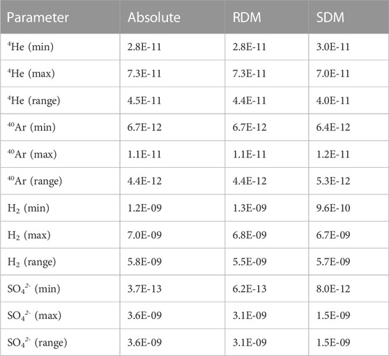
TABLE 4. Comparing the minimum, maximum, and production rates and ranges for three approaches: A) The absolute upper and lower values calculated using maximum and/or minimum values from the input ranges given in Table 1. B) The values generated by the RDM. C) The values generated by the SDM. The RDM and SDM ranges for each element are plotted on Figure 1. Both model results represent 1,000,000 values as discussed in the main text and the maximum and minimum values are also provided in Table 2. These results demonstrate that the RDM generates ranges which are most consistent with those calculated by taking the upper/lower values from the ranges. All production rates are in moles per bulk m³ per year.

Table 4, shows that the RDM approach generates production ranges comparable to the absolute ranges calculated by taking the extreme values within the range from 1,000,000 generated values. Specifically, this approach results in 98% (⁴He), 100% (⁴⁰Ar), 94% (H₂), and 86% (SO₄^2-) agreement in the ‘absolute’ calculated ranges. For the SDM, the ranges are more variable compared to the absolute range, and show 88% (⁴He), 119% (⁴⁰Ar), 98% (H₂), and 43% (SO₄^2-) agreement with the absolute values. With respect to SO₄^2-, this variability in the range is again due to the decreased probability of extreme values being selected, which is amplified by having the greatest number of input parameters. At the same time, the SDM allows for 0.3% of the values to lie outside of the specified range for all variables (except pyrite abundance and sulfide surface area). As a consequence, the expectation is that with a sufficiently large sample size this model should actually generate a slightly larger range compared to calculating production using the max or min values from the ranges. This is observed here in the case of ⁴⁰Ar, where the production primarily depends only on the potassium content and the bulk rock density (Eqs 2, 3), and so requires the least number of ‘outliers’ to produce such an enhanced range. This demonstrates then how the number of production rates generated via the SDM Monte Carlo approach must scale as a function of number of input parameters in order to fully reflect the possible upper and lowermost production rates. The same is applicable for the RDM, but the lack of biasing of the values towards a centralized value means fewer numbers will need to be generated before the maximum range reflects that of the maximum input parameters. In contrast to SDM, the RDM approach is more effective at generating a production range in line with the number of input parameters for ⁴He, ⁴⁰Ar, H₂, and SO₄^2- over 1,000,000 randomly generated production rates. In both cases however, simply comparing the Monte Carlo generated ranges to an absolute range calculated deterministically by taking the maximum or minimum value from each input parameter as appropriate provides a straightforward basis for evaluating the number of model outputs required to accurately reflect the ‘true’ maximum range.

Finally, even in cases where neither model reflects the maximum and minimum possible production rates from the input parameters, they provide insight into the likelihood (probability) of the estimated production rates and ranges. Taking SO₄^2- production as an example, although the absolute production range from the input parameters may vary by 3.6E-09 mol per bulk m³ per year, the RDM and the SDM both predict ranges of 3.1E-09 and 1.5E-09 mol per bulk m³ per year respectively from 1 million generated values. Essentially this gives a minimum confidence for these ranges of 99.9999% (with less than 1 in a million values falling outside this calculated range). The best range to use then depends on whether there is sufficient data on the input parameters to determine whether they are normally distributed or not, which is discussed in more detail in section 5.3.

5 Discussion

5.1 Comparison of Monte Carlo approach to previous state of the literature

5.1.1 ⁴He and ⁴⁰Ar production rates

The average estimated production and ranges for ⁴He, ⁴⁰Ar, H₂, and SO₄^2- generated by both Monte Carlo models (Figure 1; Table 2) are generally consistent with the previous ranges published for Kidd Creek Observatory by Warr et al. (2019) and Li et al. (2016). There are several key differences between the previous estimates and those presented here however. In the case of ⁴He and ⁴⁰Ar, the Monte Carlo generated mean production rates are both slightly lower than those of Warr et al. (2019), although the two sets of values agree within the (albeit large) maximum production ranges (horizontal black arrows). The lower mean values from the Monte Carlo approach arise because the radioelement concentration range used here spans from 0.91–2.00 ppm (U), 4.31–9.00 ppm (Th), and (1.48%–2% (K), while in the previous study only the uppermost values in these ranges were used. As a result, the average radioelement concentrations and the dependent noble gas production rates are inevitably somewhat lower here. In contrast, the very largest (most extreme) estimate of production rates from the Monte Carlo models are larger than those of Warr et al. (2019), principally due to the Monte Carlo technique integrating a range of rock density values (2.7–3.3 g/cm³) rather than the single value of 2.7 g/cm³ used by Warr et al. The net effect of this greater integration of lithological variation in the Monte Carlo approach means that a lithology with the same radioelement concentration by weight but a greater overall density will result in a higher radioelement abundance per m³ and higher predicted production of radiogenic noble gases per bulk rock volume. This combinatorial variable effect, coupled with the inherent variability in radioelement distribution, are the primary controls on production of these elements and can only be integrated in a coupled fashion using a methodology which incorporates Monte Carlo-based approaches—this ability to simultaneously incorporate lithological and elemental variation is a major advance of this new approach to these predictions and calculations.

5.1.2 H₂ production rates and ratios

For H₂ production by radiolysis (Figure 1), the mean production rates and ranges are noticeably lower than those from Warr et al. (2019) although they just overlap within uncertainty at the lower end of the 2019 estimates (Figure 1). The reasons for this revised lower estimate here are twofold: Firstly, as demonstrated in Eqs 4, 5, radioelement concentration is a primary control on H₂ production. As highlighted already for ⁴He and ⁴⁰Ar, only the uppermost radioelement concentrations were applied in Warr et al. (2019), contributing to the higher H₂ production rates previously reported therein. Secondly, the production of H₂, and therefore resultant ratios of H₂ to radiogenic ⁴He and ⁴⁰Ar (e.g., H₂/⁴He), are also highly dependent on porosity (Sherwood Lollar et al., 2014; Warr et al., 2019) which was incorporated using a slightly different approach in Warr et al. (2019). Specifically, in Warr et al. (2019), this dependence was applied to show that the average crustal production ratios for H₂/⁴He and H₂/⁴⁰Ar scale as a function of porosity from 127 to 107; to 832-701, respectively as porosity values of 1.04%–0.88% were considered. Warr et al. (2019) then multiplied these ratios by the modelled ⁴He and ⁴⁰Ar production to estimate radiolytic H₂ production. Comparing H₂/⁴He and H₂/⁴⁰Ar ratios from the Monte Carlo approaches to Warr et al. (2019) (Figure 2) shows agreement between this study and the 2019 results, but, once again, the 2019 values skew to higher estimated ratios, this time due to Warr et al. (2019) applying average global crustal production rates rather than site specific values. The Monte Carlo approach meanwhile incorporates both a wider range of radioelements, as well as the site-specific variability in porosity. While that inevitably produces a wider range of estimates, the power of the approach is that is also constrains the most probable value (mean) in a way not previously possible. In doing so, it reveals that the in situ H₂/⁴He and H₂/⁴⁰Ar production ratios at Kidd Creek Observatory are moderately lower than would be predicted based simply on average crust. This, coupled with the revised-down estimates of ⁴He and ⁴⁰Ar (due to the lower radioelement concentrations in the MC) results in the overall lower, yet more representative, H₂ production based on the site-specific parameters modelled using Monte Carlo models.

FIGURE 2

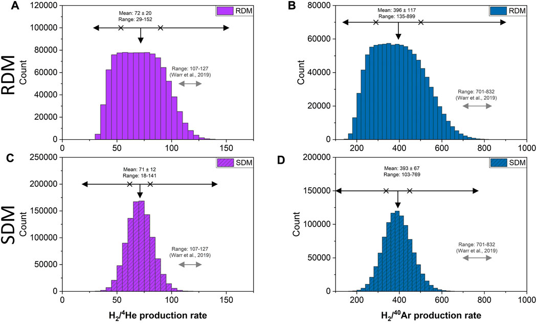
FIGURE 2. H₂/⁴He and H₂/⁴⁰Ar production ratios determined via the RDM Monte Carlo approach (A,B) and the SDM Monte Carlo approach (C,D) respectively. Each ratio was derived per cycle based on production of H₂, ⁴He, and ⁴⁰Ar generated via the Monte Carlo approach to calculate the probabilistic distribution of H₂/⁴He and H₂/⁴⁰Ar production ratios. As with Figure 1 the black horizontal arrows represent the range (maximum-minimum), the vertical arrows represent the average (mean), and the crosses represent the associated standard deviation (1 σ). The range of previous ratios used in Warr et al. (2019) are plotted as grey horizontal arrows for context.

5.1.3 SO₄^2- production rates

The estimates of SO₄^2- production via indirect radiolysis of pyrite (IROP) presented here are in agreement with those of Li et al. (2016), but both the RDM and SDM models are capable of providing the more powerful information of a most probable mean estimate, while also significantly reducing the estimated range compared to the previous study, particularly for the SDM Monte Carlo Approach (Figure 1). The reasons for this, as discussed in detail in Section 3.2, are due to sulfate production having the greatest number of input parameters, and so the range is reduced due to the decreased probability of multiple extreme values being selected. Instead, the range presented here more accurately is a function of the confidence limits with this range here representing the 99.9999% confidence (or less than 1 in 1,000,000). With respect to sulfate production then, while the previous study presented a relatively large range, this model demonstrates the ability to incorporate multiple parameters to efficiently calculate the most probable production rate along with an associated standard deviation. With a sufficiently high number of generated values, it can additionally provide constraints on the probability of numbers falling within a maximum and minimum range generated from the data. Consequently, the Monte Carlo approach applied here provides a means to generate the most probable production rates and provide considerably tighter constraints on in situ SO₄^2- production estimates.

5.1.4 Comparison summary

This study demonstrates two critical findings for the Monte Carlo approach applied to model production of H₂, ⁴He, ⁴⁰Ar, and SO₄^2-. First, this study demonstrates that both RDM and SDM can reproducibly estimate the most probable production rates and associated uncertainties at the 1 σ confidence level for a given system within 100,000 data being generated. These robust production rates incorporate the inherent variability in all input parameters simultaneously for a natural system. Secondly, this approach provides a basis to reevaluate the absolute production ranges for each chemical species (based on the uppermost and lowermost production) as a function of probability.

5.2 The importance of each parameter range via statistical experiments

An additional benefit of the Monte Carlo modelling approaches is that the relative importance and model sensitivity of each defined input range on the output can be quantitatively evaluated. This can be demonstrated by a series of statistical experiments that sequentially replace each input parameter range with a single, mid-point value and record the net decrease in the standard deviation of the mean production values. Applying this approach results in the greatest reduction in the standard deviations for the input ranges which have the most significant impact, and vice versa. The results of this are presented in Table 5 where the percentages represent the decrease in the original standard deviation caused by replacing the range with a single value.

TABLE 5

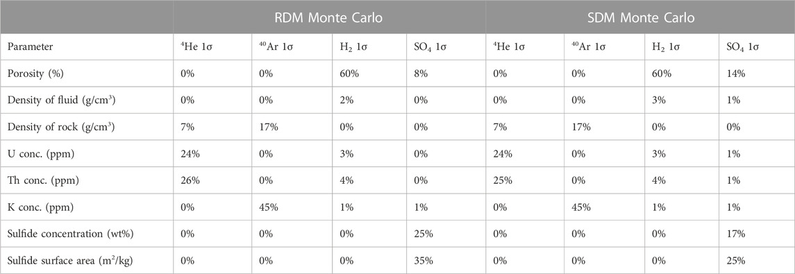
TABLE 5. The relative effect of each variable on the associated standard deviation associated with the production rates of each element. Here the relative importance of each input range on the standard deviation was evaluated for both models. The values given here represent the percentage decrease in the original standard deviations that result from changing the input parameter range to a fixed, mid-point value. Due to the combinatorial effect in multiparameter space the percentages do not add up to 100%. For example, replacing the K concentration or rock density with a single value reduces the 1 σ associated with ⁴⁰Ar by 45% and 17% respectively. However, replacing them both at the same time results in a 98% reduction in the reported ⁴⁰Ar 1 σ.

The major insights from this experimental approach are shown in Table 5. The biggest source of variability in the current model outputs from the input parameters for both ⁴He and ⁴⁰Ar production are the concentrations of the dependent radioelement concentration (U, Th for ⁴He, K for ⁴⁰Ar); followed by the density of the rock. Meanwhile, for H₂ production, the porosity range used here represents the dominant source of variability in production, with the specified density of fluids and radioelement concentration ranges in Table 1 having a relatively small effect in comparison. Lastly, for SO₄^2-, the approach provides the important insight that production the biggest variability is derived from sulfide concentration, sulfide surface area and porosity, with fluid density and radioelement concentration ranges having a minor effect. This additional ability to identify and quantify the dependence, sensitivity, and relative importance of each parameter range in the model allows additional evaluation and potentially fine tuning of the model input parameters which have the greatest impact on the production rates. This insight can define sampling or analytical strategies needed to refine estimates; or highlight why different geologic settings might return different estimates regarding habitability and radiogenic noble gas concentrations and related radiotracers (which are vital input for defining, for instance, groundwater residence times; Holland et al., 2013; Warr et al., 2018; Warr et al., 2022; Warr et al., 2023). Overall, this new approach to estimating these parameters provide a more sensitive, and hence powerful model for examining real world variability and more accurately extrapolating to global estimates.

5.3 Random distribution vs. standard distribution

This study demonstrates how ranges of input parameters can be applied to both a random (RDM) and a standard (SDM) distribution Monte Carlo approach to explore the probabilistic in situ subsurface production of key molecules (H₂, ⁴He, ⁴⁰Ar, SO₄^2-). Although both models demonstrate the ability to generate statistical probable mean estimates, associated uncertainties (standard deviation), and production rates (with an associated confidence), two key differences exist between the two approaches. Firstly, while the RDM considers all values within the input to have equal probability, the SDM considers a normally distributed input function, with mid-range values to be more likely than those approaching the upper and lower limits. Secondly, although both models essentially consider the input ranges to be upper and lower limits, in the case of the SDM these limits are ‘soft’ and values may be selected beyond this range, here at either the 3 or 5 σ level. The net effects of these differences are that the SDM generates a reduced uncertainty (standard deviation) around the mean production rate (Table 2) and generates production ranges which are considerably more sensitive to the number of input parameters needed and number of generated production values used (Section 3.2). When it comes to applying this approach to a natural system then, the question to address is how well-constrained the ranges are, and what the anticipated distribution of the data is for each variable?

Where the variable ranges are based on a very limited dataset, and are therefore relatively poorly defined, although both approaches will generate comparable mean production rates, the random distribution approach is more liable to underpredict production ranges when the numbers of model outputs are sufficiently high. This is because this approach cannot exceed the upper and lower values the way the normal distribution model can. However, the implicit assumption of a normally distributed dataset requires more careful consideration as, although many natural systems produce normally distributed populations, this is dependent on a function of scale and scope. This can be specifically highlighted here in the Kidd Creek example where both an ore zone and a non-ore zone are present in the host rock at the site. The scale of this model is such that it incorporates both of these. As a consequence, if we consider that the sulfide concentrations and surface areas are perhaps normally distributed in both zones, then combination of these then would necessarily be, at its most simple, bimodal. Alternatively, there may be a continuous distribution with a low probability of high-grade ore better represented by a log-normal distribution function. As a consequence, applying a normal distribution in this scenario may not adequately consider the natural variability in this parameter, even at this site location, resulting in standard deviations in production rates which are lower than they realistically might be. On the other hand, where a variable can be considered reasonably homogeneous at the temporal and spatial resolution being considered (a hydrogeologic term referred to as “Representative Elemental Volume, e.g., Freeze and Cherry, 1979; Bear, 1988; Adeleye and Akanji, 2018; Gilevska et al., 2021) then a normal distribution could reasonably apply which would be more reflective of the in situ variability associated with this (and comparable) input parameters.

Though the two model approaches evaluated here were either fully randomly distributed, or fully normally distributed, that there is no a priori need for all input parameters to be treated identically. While some parameters (such as the example of sulfide concentrations previously) may be more heterogeneous even at a single locality, others (such as for instance fluid density, are more likely to be homogeneous). Applying an advanced ‘hybrid’ model approach can incorporate both types of variability by treating some of the input parameters as being normally distributed, and others as randomly distributed. As a result, a careful review is needed for each of the input parameters as to whether they have individually reached the Representative Elemental Volume which reflects the scale and scope at which the variable can be considered as homogenous (e.g., Freeze and Cherry, 1979; Bear, 1988; Adeleye and Akanji, 2018; Gilevska et al., 2021). This can be evaluated by comparing the inherent variability of any parameter with the associated uncertainty. Where variability is smaller than any associated uncertainty at the system scale of interest these parameters are considered homogenous (Gilevska et al., 2019; Gilevska et al., 2021) and consequently can be modelled via the normal distribution approach. Alternatively, when this approach indicates that the variable is heterogenous for the system and scale of interest then a random distribution based on the considered maximum and minimum values will be more appropriate. In this scenario, the corresponding increased standard deviation which results from using random distributions will more reasonably reflect the increased uncertainty introduced by incorporating a heterogenous variable. Likewise, where the range for a given variable is likely to be considerable, as demonstrated in our example by pyrite abundance and sulfide surface area, alternative distribution functions may be evaluated and applied, such as inverse normal distribution or log-normal distributions, as appropriate.

5.4 Applications and implications

This parameterized Monte Carlo approach is essential for generating models which are capable of factoring in natural variability at multiple scales to estimate production of critical elements reflective of in situ conditions, especially where uncertainty may exist in one or all of the input parameters. This approach provides means to quantify this uncertainty, and evaluate its relative significance against other variables, an advance previously not possible for deterministic approaches predominantly used to date in the literature. One area of research which will significantly benefit from this type of next-generation model includes refining estimates of subsurface fluid residence times, as this approach allows realistic and site-specific physico-chemical parameters to be fully incorporated when estimating radiogenic noble gas and related radiotracer production rates (e.g., Holland et al., 2013; Heard et al., 2018; Warr et al., 2018; Warr et al., 2022; Warr et al., 2023). Improving residence time estimates, coupled with refined models of production of related bioavailable components are vital for advancing existing models of subsurface habitability. To date, significant research has focused on evaluating the role of radiolytic-driven cycling of hydrogen and sulfur in supporting chemosynthetic ecosystems (e.g., Lin et al., 2005b; Lin et al., 2006; Chivian et al., 2008; D’Hondt et al., 2009; Sherwood Lollar et al., 2014; Dzaugis et al., 2016; Li et al., 2016, 2022; Telling et al., 2017; Warr et al., 2019; Bomberg et al., 2021; Sauvage et al., 2021; Nisson et al., 2023). Most recently, research has expanded this aspect to consider cycling of other associated critical bio-elements, such as nitrogen, and simple organic molecules (e.g., Silver et al., 2012; Adam et al., 2021; Li et al., 2021; Sherwood Lollar et al., 2021; Vandenborre et al., 2021; Karolytė et al., 2022), and to evaluate alternative habitability models beyond Earth on other worlds such as Mars, Enceladus, and Europa (Onstott et al., 2006; Bouquet et al., 2017; Dzaugis et al., 2018; Tarnas et al., 2018; 2021). However, underpinning this entire research field is the fundamental requirement of accurately being able to model representative radiolytic production of elements within the system(s). This has resulted in a recent shift from deterministic towards a probabilistic approach, demonstrated both here via Monte Carlo approach and by incorporating additional statistical-based approaches (e.g., Bayesian modelling - Gallagher et al., 2009; Karolytė et al., 2022) to generate the next-generation of models to incorporate variability within natural systems. These next-generation models are essential in order to provide more quantifiable and probabilistic approach to these estimates, less subject to inherent variability in the input parameters and hence more representative regional/global estimates necessary to understand the significance of these processes for Earth, Mars, or the other moons and planets in the Solar System.

Lastly, this approach can be applied to the field of economic resource development, specifically for helium, which is essential for modern medical, research, and industry application, and hydrogen, which represents a prospective, low-carbon alternative energy source (Bartels et al., 2010; Hanley et al., 2018; Danabalan et al., 2022; Milkov, 2022; Warr et al., 2022). To date, the exploration techniques to identify the processes surrounding formation, accumulation, and storage of economic reservoirs remain preliminary and require development (Warr et al., 2019; 2022; Cheng et al., 2021; Danabalan et al., 2022; Milkov, 2022; Cheng et al., 2023). Applying next-generation models, such as the one presented here, which can be applied to calculate production on local to regional scales, are therefore essential for implementing refined and effective strategies to identify and exploit these critical resources and ensure 21st century needs are met.

6 Conclusion

This study demonstrates a novel approach to incorporate the effects of natural variability of controlling parameters on subsurface radiolytic production models by integrating a computationally inexpensive Monte Carlo technique to recent radiolytic/radiogenic models for the first time. Specifically, we apply a Monte Carlo-based approach to Kidd Creek Observatory in Canada and compare estimated production of H₂, ⁴He, ⁴⁰Ar, SO₄^2- with previous models that used straightforward deterministic approaches (Li et al., 2016; Warr et al., 2019). This novel modelling technique outlined here effectively demonstrates how the natural variability associated with each parameter can be simultaneously considered to generate refined next-generation models which can be applied and/or scaled for natural systems to produce statistically probable best estimates (mean values), as well as quantitative range for upper and lower values for in situ estimates of H₂, ⁴He, ⁴⁰Ar, SO₄^2- (and related elements). Due to its decadal compilation of an unprecedented multi-parameter dataset from the deep subsurface, the Kidd Creek Observatory is useful for this proof in principle of the approach bas the MC results can be compared in principle to previously calculated estimates. We anticipate this MC approach can now be applied generally to the large number of other subsurface systems around the globe that are less well characterized, in order to generate estimates of ⁴He, H₂, ⁴⁰Ar and SO₄^2- production with improved confidence in both the range of estimates (maxima and minimum) and most probable values, even at sites that may be much less well-studied than Kidd Creek. Similarly, this approach allows hypothesis testing and estimation of production of these critical parameters for resource formation, habitability models in the context of not only terrestrial-based studies, but also in planetary sciences and astrobiological studies focusing on Mars, or the moons of Jupiter and Saturn and beyond.

Data availability statement

The raw data supporting the conclusion of this article will be made available by the authors, without undue reservation.

Author contributions

OW and BSL contributed to conception and design of the study. OW and MS constructed and validated the Monte Carlo model. OW wrote the first draft of the manuscript. All authors contributed to manuscript revision and approved the submitted version.

Funding

This study was financially supported by the Nuclear Waste Management Organisation (NWMO), with additional funding provided by the Natural Sciences and Engineering Research Council of Canada Discovery and NFREF grants. Sherwood Lollar is a Director of the CIFAR Earth 4D Subsurface Science and Exploration program.

Conflict of interest

The authors declare that the research was conducted in the absence of any commercial or financial relationships that could be construed as a potential conflict of interest.

Publisher’s note

All claims expressed in this article are solely those of the authors and do not necessarily represent those of their affiliated organizations, or those of the publisher, the editors and the reviewers. Any product that may be evaluated in this article, or claim that may be made by its manufacturer, is not guaranteed or endorsed by the publisher.

References

Adam, Z. R., Fahrenbach, A. C., Jacobson, S. M., Kacar, B., and Zubarev, D. Y. (2021). Radiolysis generates a complex organosynthetic chemical network. Sci. Rep. 11, 1743–1810. doi:10.1038/s41598-021-81293-6

PubMed Abstract | CrossRef Full Text | Google Scholar

Adeleye, J. O., and Akanji, L. T. (2018). Pore-scale analyses of heterogeneity and representative elementary volume for unconventional shale rocks using statistical tools. J. Pet. Explor. Prod. Technol. 8, 753–765. doi:10.1007/s13202-017-0377-4

CrossRef Full Text | Google Scholar

Altair, T., De Avellar, M. G. B., Rodrigues, F., and Galante, D. (2018). Microbial habitability of Europa sustained by radioactive sources. Sci. Rep. 8, 260–268. doi:10.1038/s41598-017-18470-z

PubMed Abstract | CrossRef Full Text | Google Scholar

Aquilina, L., de Dreuzy, J.-R., Bour, O., and Davy, P. (2004). Porosity and fluid velocities in the upper continental crust (2 to 4 km) inferred from injection tests at the Soultz-sous-Forêts geothermal site. Geochim. Cosmochim. Acta 68, 2405–2415. doi:10.1016/j.gca.2003.08.023

CrossRef Full Text | Google Scholar

Ballentine, C. J., and Burnard, P. G. (2002). Production, release and transport of noble gases in the continental crust. Rev. Mineral. Geochem. 47, 481–538. doi:10.2138/rmg.2002.47.12

CrossRef Full Text | Google Scholar

Bartels, J. R., Pate, M. B., and Olson, N. K. (2010). An economic survey of hydrogen production from conventional and alternative energy sources. Int. J. Hydrogen Energy 35, 8371–8384. doi:10.1016/j.ijhydene.2010.04.035

CrossRef Full Text | Google Scholar

Bear, J. (1988). Dynamics of fluids in porous media. Courier Corporation.

Google Scholar

Benedetti, L., Claeys, F., Nopens, I., and Vanrolleghem, P. A. (2011). Assessing the convergence of LHS Monte Carlo simulations of wastewater treatment models. Water Sci. Technol. 63, 2219–2224. doi:10.2166/WST.2011.453

PubMed Abstract | CrossRef Full Text | Google Scholar

Berger, B. R., Bleeker, W., van Breemen, O., Chapman, J. B., Peter, J. M., Layton-Matthews, D., et al. (2011). Results from the targeted geoscience initiative III kidd–munro project. Open File Rep. 6258.

Google Scholar

Bethke, C. M. (1985). A numerical model of compaction-driven groundwater flow and heat transfer and its application to the paleohydrology of intracratonic sedimentary basins. J. Geophys. Res. Solid Earth 90, 6817–6828. doi:10.1029/JB090iB08p06817

CrossRef Full Text | Google Scholar

Blair, C. C., D’Hondt, S., Spivack, A. J., and Kingsley, R. H. (2007). Radiolytic hydrogen and microbial respiration in subsurface sediments. Astrobiology 7, 951–970. doi:10.1089/AST.2007.0150

PubMed Abstract | CrossRef Full Text | Google Scholar

Bleeker, W., and Parrish, R. R. (1996). Stratigraphy and U-Pb zircon geochronology of Kidd Creek: Implications for the formation of giant volcanogenic massive sulphide deposits and the tectonic history of the Abitibi greenstone belt. Can. J. Earth Sci. 33, 1213–1231. doi:10.1139/e96-092

CrossRef Full Text | Google Scholar

Bomberg, M., Miettinen, H., Kietäväinen, R., Purkamo, L., Ahonen, L., and Vikman, M. (2021). “Chapter 3 - microbial metabolic potential in deep crystalline bedrock,” in The microbiology of nuclear Waste disposal. Editors J. R. Lloyd, and A. Cherkouk (Elsevier), 41–70. doi:10.1016/B978-0-12-818695-4.00003-4

CrossRef Full Text | Google Scholar

Boreham, C. J., Sohn, J. H., Cox, N., Williams, J., Hong, Z., and Kendrick, M. A. (2021). Hydrogen and hydrocarbons associated with the neoarchean frog’s leg gold camp, yilgarn craton, western Australia. Chem. Geol. 575, 120098. doi:10.1016/j.chemgeo.2021.120098

CrossRef Full Text | Google Scholar

Bouquet, A., Glein, C. R., Wyrick, D., and Waite, J. H. (2017). Alternative energy: Production of H₂ by radiolysis of water in the rocky cores of icy bodies. Astrophys. J. Lett. 840, L8. doi:10.3847/2041-8213/aa6d56

CrossRef Full Text | Google Scholar

Bucher, K., and Stober, I. (2010). Fluids in the upper continental crust. Geofluids 10, 241–253. doi:10.1111/j.1468-8123.2010.00279.x

CrossRef Full Text | Google Scholar

Cheng, A., Sherwood Lollar, B., Gluyas, J. G., and Ballentine, C. J. (2023). Primary N₂–He gas field formation in intracratonic sedimentary basins. Nature 615, 94–99. doi:10.1038/s41586-022-05659-0

PubMed Abstract | CrossRef Full Text | Google Scholar

Cheng, A., Sherwood Lollar, B., Warr, O., Ferguson, G., Idiz, E., Mundle, S. O. C., et al. (2021). Determining the role of diffusion and basement flux in controlling ⁴He distribution in sedimentary basin fluids. Earth Planet. Sci. Lett. 574, 117175. doi:10.1016/J.EPSL.2021.117175

CrossRef Full Text | Google Scholar

Chivian, D., Brodie, E. L., Alm, E. J., Culley, D. E., Dehal, P. S., DeSantis, T. Z., et al. (2008). Environmental genomics reveals a single-species ecosystem deep within Earth. Science 322, 275–278. doi:10.1126/science.1155495

PubMed Abstract | CrossRef Full Text | Google Scholar

Crutchfield, J. P. (1994). The calculi of emergence: Computation, dynamics and induction. Phys. D. Nonlinear Phenom. 75, 11–54. doi:10.1016/0167-2789(94)90273-9

CrossRef Full Text | Google Scholar

Danabalan, D., Gluyas, J. G., Macpherson, C. G., Abraham-James, T. H., Bluett, J. J., Barry, P. H., et al. (2022). The principles of helium exploration. Pet. Geosci. 28. doi:10.1144/petgeo2021-029

CrossRef Full Text | Google Scholar

Davis, D. W., Schandl, E. S., and Wasteneys, H. A. (1994). U-Pb dating of minerals in alteration halos of superior province massive sulfide deposits: Syngenesis versus metamorphism. Contrib. Mineral. Petrol. 115, 427–437. doi:10.1007/BF00320976

CrossRef Full Text | Google Scholar

D’Hondt, S., Spivack, A. J., Pockalny, R., Ferdelman, T. G., Fischer, J. P., Kallmeyer, J., et al. (2009). Subseafloor sedimentary life in the south pacific gyre. Proc. Natl. Acad. Sci. 106, 11651–11656. doi:10.1073/pnas.0811793106

CrossRef Full Text | Google Scholar

Dzaugis, M. E., Spivack, A. J., Dunlea, A. G., Murray, R. W., and D’Hondt, S. (2016). Radiolytic hydrogen production in the subseafloor basaltic aquifer. Front. Microbiol. 7, 76. doi:10.3389/fmicb.2016.00076

PubMed Abstract | CrossRef Full Text | Google Scholar

Dzaugis, M., Spivack, A. J., and D’Hondt, S. (2018). Radiolytic H₂ production in martian environments. Astrobiology 18, 1137–1146. doi:10.1089/ast.2017.1654

PubMed Abstract | CrossRef Full Text | Google Scholar

Flowers, R. M., Bowring, S. A., and Reiners, P. W. (2006). Low long-term erosion rates and extreme continental stability documented by ancient (U-Th)/He dates. Geology 34, 925–928. doi:10.1130/G22670A.1

CrossRef Full Text | Google Scholar

Freeze, R. A., and Cherry, J. A. (1979). Groundwater. Prentice-Hall.

Google Scholar

Gallagher, K., Charvin, K., Nielsen, S., Sambridge, M., and Stephenson, J. (2009). Markov chain Monte Carlo (MCMC) sampling methods to determine optimal models, model resolution and model choice for Earth Science problems. Mar. Pet. Geol. 26, 525–535. doi:10.1016/J.MARPETGEO.2009.01.003

CrossRef Full Text | Google Scholar

Gilevska, T., Passeport, E., Shayan, M., Seger, E., Lutz, E. J., West, K. A., et al. (2019). Determination of in situ biodegradation rates via a novel high resolution isotopic approach in contaminated sediments. Water Res. 149, 632–639. doi:10.1016/J.WATRES.2018.11.029

PubMed Abstract | CrossRef Full Text | Google Scholar

Gilevska, T., Sullivan Ojeda, A., Kümmel, S., Gehre, M., Seger, E., West, K., et al. (2021). Multi-element isotopic evidence for monochlorobenzene and benzene degradation under anaerobic conditions in contaminated sediments. Water Res. 207, 117809. doi:10.1016/J.WATRES.2021.117809

PubMed Abstract | CrossRef Full Text | Google Scholar

Gillman, E., and Gillman, M. (2019). Modelling nature: An introduction to mathematical modelling of natural systems. CABI.

Google Scholar

Guillot, L., Siitari-Kauppi, M., Hellmuth, K-H., Dubois, C., Rossy, M., and Gaviglio, P. (2000). Porosity changes in a granite close to quarry faces: Quantification and distribution by 14C-mma and Hg porosimetries. Eur. Phys. J. Ap. 9, 137–146. doi:10.1051/epjap:2000211

CrossRef Full Text | Google Scholar

Hanley, E. S., Deane, J. P., and Gallachóir, B. P. Ó. (2018). The role of hydrogen in low carbon energy futures–A review of existing perspectives. Renew. Sustain. Energy Rev. 82, 3027–3045. doi:10.1016/J.RSER.2017.10.034

CrossRef Full Text | Google Scholar

Hannington, M. D., Bleeker, W., and Kjarsgaard, I. (1999). Sulfide mineralogy, geochemistry, and ore genesis of the Kidd Creek deposit: Part I. North, central, and south orebodies. West Abitibi Subprov. Canada: Giant Kidd Creek Volcanogenic Massive Sulfide Depos, 163–224. doi:10.5382/MONO.10.07

CrossRef Full Text | Google Scholar

Heard, A. W., Warr, O., Borgonie, G., Linage, B., Kuloyo, O., Fellowes, J. W., et al. (2018). South African crustal fracture fluids preserve paleometeoric water signatures for up to tens of millions of years. Chem. Geol. 493, 379–395. doi:10.1016/j.chemgeo.2018.06.011

CrossRef Full Text | Google Scholar

Holland, G., and Gilfillan, S. (2013). “Application of noble gases to the viability of CO₂ storage,” in The noble gases as geochemical tracers. Editor P. Burnard (Springer), 177–223.

CrossRef Full Text | Google Scholar

Holland, G., Sherwood Lollar, B., Li, L., Lacrampe-Couloume, G., Slater, G. F., and Ballentine, C. J. (2013). Deep fracture fluids isolated in the crust since the Precambrian era. Nature 497, 357–360. doi:10.1038/Nature12127

PubMed Abstract | CrossRef Full Text | Google Scholar

Hopper, A., and Rice, A. (2008). Computing for the future of the planet. Phil. Trans. R. Soc. A 366, 3685–3697. doi:10.1098/rsta.2008.0124

PubMed Abstract | CrossRef Full Text | Google Scholar

Karolytė, R., Warr, O., van Heerden, E., Flude, S., de Lange, F., Webb, S., et al. (2022). The role of porosity in H₂/He production ratios in fracture fluids from the Witwatersrand Basin, South Africa. Chem. Geol. 595, 120788. doi:10.1016/J.CHEMGEO.2022.120788

CrossRef Full Text | Google Scholar

Ketchum, J. W. F., Ayer, J. A., Van Breemen, O., Pearson, N. J., and Becker, J. K. (2008). Pericontinental crustal growth of the southwestern Abitibi subprovince, Canada—U-Pb, Hf, and Nd isotope evidence. Econ. Geol. 103, 1151–1184. doi:10.2113/gsecongeo.103.6.1151

CrossRef Full Text | Google Scholar

Lefticariu, L., Pratt, L. A., LaVerne, J. A., and Schimmelmann, A. (2010). Anoxic pyrite oxidation by water radiolysis products — a potential source of biosustaining energy. Earth Planet. Sci. Lett. 292, 57–67. doi:10.1016/J.EPSL.2010.01.020

CrossRef Full Text | Google Scholar

Li, L., Li, K., Giunta, T., Warr, O., Labidi, J., and Sherwood Lollar, B. (2021). N₂ in deep subsurface fracture fluids of the Canadian Shield: Source and possible recycling processes. Chem. Geol. 585, 120571. doi:10.1016/J.CHEMGEO.2021.120571

CrossRef Full Text | Google Scholar

Li, L., Wei, S., Sherwood Lollar, B., Wing, B., Bui, T. H., Ono, S., et al. (2022). In situ oxidation of sulfide minerals supports widespread sulfate reducing bacteria in the deep subsurface of the Witwatersrand Basin (South Africa): Insights from multiple sulfur and oxygen isotopes. Earth Planet. Sci. Lett. 577, 117247. doi:10.1016/J.EPSL.2021.117247

CrossRef Full Text | Google Scholar

Li, L., Wing, B. A., Bui, T. H., McDermott, J. M., Slater, G. F., Wei, S., et al. (2016). Sulfur mass-independent fractionation in subsurface fracture waters indicates a long-standing sulfur cycle in Precambrian rocks. Nat. Commun. 7, 13252. Artn 13252. doi:10.1038/Ncomms13252

PubMed Abstract | CrossRef Full Text | Google Scholar

Lin, L. H., Hall, J., Lippmann-Pipke, J., Ward, J. A., Sherwood Lollar, B., DeFlaun, M., et al. (2005a). Radiolytic H₂ in continental crust: Nuclear power for deep subsurface microbial communities. Geochem. Geophys. Geosystems 6, 7. doi:10.1029/2004GC000907

CrossRef Full Text | Google Scholar

Lin, L. H., Slater, G. F., Sherwood Lollar, B., Lacrampe-Couloume, G., and Onstott, T. C. (2005b). The yield and isotopic composition of radiolytic H₂, a potential energy source for the deep subsurface biosphere. Geochim. Cosmochim. Acta 69, 893–903. doi:10.1016/j.gca.2004.07.032

CrossRef Full Text | Google Scholar

Lin, L. H., Wang, P. L., Rumble, D., Lippmann-Pipke, J., Boice, E., Pratt, L. M., et al. (2006). Long-term sustainability of a high-energy, low-diversity crustal biome. Science 314, 479–482. doi:10.1126/science.1127376

PubMed Abstract | CrossRef Full Text | Google Scholar

Lippmann, J., Stute, M., Torgersen, T., Moser, D. P., Hall, J. A., Lin, L., et al. (2003). Dating ultra-deep mine waters with noble gases and ³⁶Cl, Witwatersrand Basin, South Africa. Geochim. Cosmochim. Acta 67, 4597–4619. doi:10.1016/S0016-7037(03)00414-9

CrossRef Full Text | Google Scholar

Lippmann-Pipke, J., Sherwood Lollar, B., Niedermann, S., Stroncik, N. A., Naumann, R., van Heerden, E., et al. (2011). Neon identifies two billion year old fluid component in Kaapvaal Craton. Chem. Geol. 283, 287–296. doi:10.1016/j.chemgeo.2011.01.028

CrossRef Full Text | Google Scholar

Liu, B., and Liang, Y. (2017). An introduction of Markov chain Monte Carlo method to geochemical inverse problems: Reading melting parameters from REE abundances in abyssal peridotites. Geochim. Cosmochim. Acta 203, 216–234. doi:10.1016/J.GCA.2016.12.040

CrossRef Full Text | Google Scholar

Lollar, G. S., Warr, O., Telling, J., Osburn, M. R., and Sherwood Lollar, B. (2019). ‘Follow the water’: Hydrogeochemical constraints on microbial investigations 2.4 km below surface at the Kidd Creek deep fluid and deep life observatory. Geomicrobiol. J. 36, 859–872. doi:10.1080/01490451.2019.1641770

CrossRef Full Text | Google Scholar

Milkov, A. V. (2022). Molecular hydrogen in surface and subsurface natural gases: Abundance, origins and ideas for deliberate exploration. Earth-Science Rev. 230, 104063. doi:10.1016/J.EARSCIREV.2022.104063

CrossRef Full Text | Google Scholar

Moulton, B. J. A., Fowler, A. D., Ayer, J. A., Berger, B. R., and Mercier-Langevin, P. (2011). Archean subqueous high-silica rhyolite coulées: Examples from the kidd-munro assemblage in the Abitibi subprovince. Precambrian Res. 189, 389–403. doi:10.1016/j.precamres.2011.07.002

CrossRef Full Text | Google Scholar

National Academies of Sciences, Engineering, and Medicine (2019). An astrobiology strategy for the search for life in the universe. doi:10.17226/25252

CrossRef Full Text | Google Scholar

Nisson, D. M., Kieft, T. L., Drake, H., Warr, O., Sherwood Lollar, B., Ogasawara, H., et al. (2023). Hydrogeochemical and isotopic signatures elucidate deep subsurface hypersaline brine formation through radiolysis driven water-rock interaction. Geochim. Cosmochim. Acta 340, 65–84. doi:10.1016/J.GCA.2022.11.015

CrossRef Full Text | Google Scholar

Onstott, T. C., McGown, D., Kessler, J., Sherwood Lollar, B., Lehmann, K. K., and Clifford, S. M. (2006). Martian CH4: Sources, flux, and detection. Astrobiology 6, 377–395. doi:10.1089/ast.2006.6.377

PubMed Abstract | CrossRef Full Text | Google Scholar

Sakan, S., Sakan, N., Popović, A., Škrivanj, S., and Đorđević, D. (2019). Geochemical fractionation and assessment of probabilistic ecological risk of potential toxic elements in sediments using Monte Carlo simulations. Mol 24, 2145. doi:10.3390/MOLECULES24112145

CrossRef Full Text | Google Scholar

Sambridge, M., and Mosegaard, K. (2002). Monte Carlo methods in geophysical inverse problems. Rev. Geophys. 40, 3-1–3-29. doi:10.1029/2000RG000089

CrossRef Full Text | Google Scholar

Sauvage, J. F., Flinders, A., Spivack, A. J., Pockalny, R., Dunlea, A. G., Anderson, C. H., et al. (2021). The contribution of water radiolysis to marine sedimentary life. Nat. Commun. 12, 1297. doi:10.1038/s41467-021-21218-z

PubMed Abstract | CrossRef Full Text | Google Scholar

Shalizi, C. R., and Crutchfield, J. P. (2001). Computational mechanics: Pattern and prediction, structure and simplicity. J. Stat. Phys. 104, 817–879. doi:10.1023/A:1010388907793

CrossRef Full Text | Google Scholar

Sherwood Lollar, B., Frape, S. K., Weise, S. M., Fritz, P., Macko, S. A., and Welhan, J. A. (1993). Abiogenic methanogenesis in crystalline rocks. Geochim. Cosmochim. Acta 57, 5087–5097. doi:10.1016/0016-7037(93)90610-9

CrossRef Full Text | Google Scholar

Sherwood Lollar, B., Heuer, V. B., McDermott, J., Tille, S., Warr, O., Moran, J. J., et al. (2021). A window into the abiotic carbon cycle – acetate and formate in fracture waters in 2.7 billion year-old host rocks of the Canadian Shield. Geochim. Cosmochim. Acta 294, 295–314. doi:10.1016/j.gca.2020.11.026

CrossRef Full Text | Google Scholar

Sherwood Lollar, B., Onstott, T. C., Lacrampe-Couloume, G., and Ballentine, C. J. (2014). The contribution of the Precambrian continental lithosphere to global H₂ production. Nature 516, 379–382. doi:10.1038/nature14017

PubMed Abstract | CrossRef Full Text | Google Scholar

Silver, B. J., Raymond, R., Sigman, D. M., Prokopeko, M., Sherwood Lollar, B., Lacrampe-Couloume, G., et al. (2012). The origin of NO₃^- and N₂ in deep subsurface fracture water of South Africa. Chem. Geol. 294–295, 51–62. doi:10.1016/j.chemgeo.2011.11.017

PubMed Abstract | CrossRef Full Text | Google Scholar

Stober, I., and Bucher, K. (2007). Hydraulic properties of the crystalline basement. Hydrogeol. J. 15, 213–224. doi:10.1007/s10040-006-0094-4

CrossRef Full Text | Google Scholar

Stober, I. (2011). Depth- and pressure-dependent permeability in the upper continental crust: Data from the Urach 3 geothermal borehole, southwest Germany. Hydrogeol. J. 19, 685–699. doi:10.1007/s10040-011-0704-7

CrossRef Full Text | Google Scholar

Stober, I. (1997). Permeabilities and chemical properties of water in crystalline rocks of the black forest, Germany. Aquat. Geochem. 3, 43–60. doi:10.1023/A:1009623432059

CrossRef Full Text | Google Scholar

Tarnas, J. D., Mustard, J. F., Sherwood Lollar, B., Bramble, M. S., Cannon, K. M., Palumbo, A. M., et al. (2018). Radiolytic H₂ production on Noachian Mars: Implications for habitability and atmospheric warming. Earth Planet. Sci. Lett. 502, 133–145. doi:10.1016/j.epsl.2018.09.001

CrossRef Full Text | Google Scholar

Tarnas, J. D., Mustard, J. F., Sherwood Lollar, B., Stamenković, V., Cannon, K. M., Lorand, J.-P., et al. (2021). Earth-like habitable environments in the subsurface of Mars. Astrobiology 21, 741–756. doi:10.1089/ast.2020.2386

PubMed Abstract | CrossRef Full Text | Google Scholar

Telling, J., Voglesonger, K., Sutcliffe, C. N., Lacrampe-Couloume, G., Edwards, E., and Sherwood Lollar, B. (2017). Bioenergetic constraints on microbial hydrogen utilization in precambrian deep crustal fracture fluids. Geomicrobiol. J. 1, 108–119. doi:10.1080/01490451.2017.1333176

CrossRef Full Text | Google Scholar

Thurston, P. C., Ayer, J. A., Goutier, J., and Hamilton, M. A. (2008). Depositional gaps in Abitibi greenstone belt stratigraphy: A key to exploration for syngenetic mineralization. Econ. Geol. 103, 1097–1134. doi:10.2113/gsecongeo.103.6.1097

CrossRef Full Text | Google Scholar

Vandenborre, J., Truche, L., Costagliola, A., Craff, E., Blain, G., Baty, V., et al. (2021). Carboxylate anion generation in aqueous solution from carbonate radiolysis, a potential route for abiotic organic acid synthesis on Earth and beyond. Earth Planet. Sci. Lett. 564, 116892. doi:10.1016/J.EPSL.2021.116892

CrossRef Full Text | Google Scholar

Ventura, G. T., Kenig, F., Reddy, C. M., Schieber, J., Frysinger, G. S., Nelson, R. K., et al. (2007). Molecular evidence of Late Archean archaea and the presence of a subsurface hydrothermal biosphere. Proc. Natl. Acad. Sci. 104, 14260–14265. doi:10.1073/pnas.0610903104

PubMed Abstract | CrossRef Full Text | Google Scholar

Wang, Z., Yin, Z., Caers, J., and Zuo, R. (2020). A Monte Carlo-based framework for risk-return analysis in mineral prospectivity mapping. Geosci. Front. 11, 2297–2308. doi:10.1016/J.GSF.2020.02.010

CrossRef Full Text | Google Scholar

Warr, O., Ballentine, C. J., Mu, J., and Masters, A. (2015). Optimizing noble gas-water interactions via Monte Carlo simulations. J. Phys. Chem. B 119, 14486–14495. doi:10.1021/acs.jpcb.5b06389

PubMed Abstract | CrossRef Full Text | Google Scholar

Warr, O., Ballentine, C. J., Onstott, T. C., Nisson, D. M., Kieft, T. L., Hillegonds, D. J., et al. (2022). ⁸⁶Kr excess and other noble gases identify a billion-year-old radiogenically-enriched groundwater system. Nat. Commun. 13, 3768. doi:10.1038/s41467-022-31412-2

PubMed Abstract | CrossRef Full Text | Google Scholar

Warr, O., Giunta, T., Ballentine, C. J., and Sherwood Lollar, B. (2019). Mechanisms and rates of ⁴He, ⁴⁰Ar, and H₂ production and accumulation in fracture fluids in Precambrian Shield environments. Chem. Geol. 530, 119322. doi:10.1016/j.chemgeo.2019.119322

CrossRef Full Text | Google Scholar

Warr, O., Giunta, T., Onstott, T. C., Kieft, T. L., Harris, R. L., Nisson, D. M., et al. (2021a). The role of low-temperature ¹⁸O exchange in the isotopic evolution of deep subsurface fluids. Chem. Geol. 561, 120027. doi:10.1016/j.chemgeo.2020.120027

CrossRef Full Text | Google Scholar

Warr, O., Sherwood Lollar, B., Fellowes, J., Sutcliffe, C. N., McDermott, J. M., Holland, G., et al. (2018). Tracing ancient hydrogeological fracture network age and compartmentalisation using noble gases. Geochim. Cosmochim. Acta 222, 340–362. doi:10.1016/j.gca.2017.10.022

CrossRef Full Text | Google Scholar

Warr, O., Smith, N. J. T., and Sherwood Lollar, B. (2023). Hydrogeochronology: Resetting the timestamp for subsurface groundwaters geochim. Cosmochim. Acta in press.

Google Scholar

Warr, O., Young, E. D., Giunta, T., Kohl, I. E., Ash, J. L., and Sherwood Lollar, B. (2021b). High-resolution, long-term isotopic and isotopologue variation identifies the sources and sinks of methane in a deep subsurface carbon cycle. Geochim. Cosmochim. Acta 294, 315–334. doi:10.1016/j.gca.2020.12.002

CrossRef Full Text | Google Scholar

Wilensky, U., and Rand, W. (2015). An introduction to agent-based modeling: Modeling natural, social, and engineered complex systems with NetLogo. MIT Press.

Google Scholar

Yi, R., Hongo, Y., Yoda, I., Adam, Z. R., and Fahrenbach, A. C. (2018). Radiolytic synthesis of cyanogen chloride, cyanamide and simple sugar precursors. ChemistrySelect 3, 10169–10174. doi:10.1002/SLCT.201802242

CrossRef Full Text | Google Scholar