Detection of electromagnetic anomalies over seismic regions during two strong (MW > 5) earthquakes

1 Introduction

Earthquakes (EQs) are natural disasters that severely impact human life. For this reason, the scientific Community has always been interested in mitigating their effects for the purposes of life preservation and boosting of economic resilience. Over the last two decades, several works have shown that, before strong earthquakes, characteristic EM signals can be detected both in the extremely low (ELF) and very low frequency (VLF) bands, usually in the atmosphere and ionosphere (Molchanov and Hayakawa, 1998; Pulinets and Boyarchuk, 2004; Hayakawa, 2015; Pulinets et al., 2022). The more frequently EM signals possibly induced by EQs are detected, the hotter the topic of (even short-term) EQ forecasting becomes.

It is well known that solar activity can influence the ionosphere, leading to the so-called solar wind/magnetosphere/ionosphere coupling (Villante and Piersanti, 2011; Piersanti et al., 2020a). However, the ionospheric medium can also be influenced by waves generated in low atmospheric layers and propagating upwards (Hines, 1960). Recent works have shown that low-frequency EM waves can penetrate the lower ionosphere and be observed by satellites at low Earth orbit (LEO) (Cohen and Inan, 2012; Zhao et al., 2019). Before the launch of the DEMETER (Detection of Electromagnetic Emissions Transmitted from Earthquake Regions) satellite in 2004 (Lagoutte et al., 2006), all EQ-related analysis would be carried out using data from non-dedicated satellites. The DEMETER mission has paved the way for the development of specific investigations, which have been resulting in the detection of several EQ-induced emissions since the end of the 2000s (Němec et al., 2009; Zhang et al., 2012; Walker et al., 2013; Zhang et al., 2013; Bertello et al., 2018; Zhima et al., 2020).

At present, the CSES-01 satellite represents the most advanced LEO mission for the investigation of seismo-induced phenomena in the near-Earth electromagnetic environment (Shen et al., 2018). The CSES mission provides two remarkable benefits. On the one hand, CSES-01 is just the first element of a scheduled constellation intended for optimized coverage of the Earth’s seismic regions. On the other hand, the CSES-01 satellite hosts nine payloads, which ensure the possibility of a multi-instrumental approach to the analysis of the ionospheric environment. Launched in February 2018, CSES-01 has already provided systematic evidence of EM anomalies correlated with seismic activity [e.g., (Piersanti et al., 2020b; Wang et al., 2022; Zong et al., 2022)].

In order to give a formal frame to such observations, a few models have been proposed to justify the coupling between lithosphere, atmosphere and ionosphere. One of the most promising is the MILC model (Carbone et al., 2021), which is based on the concept of the emission and propagation of an acoustic gravity wave (AGW). AGWs are characterized by a period of approximately 5 min–10 h, and a wavelength of 10 m–100 km (see (Carbone et al., 2021) and references therein). These oscillations arise around the EE, inducing a pressure gradient in the atmosphere, which in turn triggers disturbances in the ionosphere (Molchanov et al., 2001; Miyaki et al., 2002; Muto et al., 2009; Hayakawa et al., 2011). Various observations of EQ-induced AGWs have been reported so far in the literature (Mikumo and Watada, 2010; Piersanti et al., 2020b; D’Angelo et al., 2022a). That is why an accurate procedure for the identification of the ionospheric anomalies is required for better understanding of the physics behind the lithosphere/atmosphere/ionosphere coupling, and for model validation.

A crucial step in the identification of anomalies consists in the definition of the statistical distribution of the ionospheric EM-wave energy in the absence of seismic activity and any other additional forcing. The determination of this characteristic background cannot be avoided when looking for extreme reliability in the search for pre-seismic/co-seismic phenomena. In this scenario, a signal can be defined as anomalous if it statistically differs from the background.

In this paper, we propose a new technique to compute the ionospheric EM background above seismic regions. Our algorithm is based on the application of the Fast Iterative Filtering [FIF, (Cicone and Zhou, 2021)] method of signal analysis, and on a multiscale statistical analysis of EM observations. A set of ionospheric EM background maps over seismic regions has been generated using CSES-01 electric- and magnetic-field observations from 2019 to 2021, and then compared with signals detected over any EE just before the EQ occurrence in order to discriminate anomalies from typical ionospheric features (at the appropriate geomagnetic conditions).

This technique has been tested against two different seismic events, which struck Haiti on 14 August 2021 and Crete on 27 September 2021, respectively. The reason behind this selection is twofold. First, both the EQs occurred in 2021, thus matching CSES-01’s window of data availability. In addition, the two earthquakes occurred under very different geomagnetic conditions, which enables an assessment of the role of solar forcing in this type of analysis.

The arrangement of the manuscript is as follows: Section 2 contains data and methods used for the analysis; Section 3 presents the two case-event tests; finally, the discussion about obtained results is reported in Section 4.

2 Data and methods

The following section describes the techniques applied for the development of the algorithm, as well as the dataset used to test it.

2.1 CSES data

The calculation of the ionospheric EM background is based on data from the CSES (China Seismo-Electromagnetic Satellite) mission (Shen et al., 2018). It is a mission dedicated to the study of possible temporal and spatial correlations between the occurrence of seismic events (at medium and strong magnitudes) and iono/magnetospheric EM perturbations, plasma variations, and particle precipitation from the Van Allen belts. The first CSES satellite was launched on a Sun-synchronous quasi-polar orbit (altitude: ∼500 km) from the Jiuquan Launch Center by means of a Long March 2D carrier rocket in 2018. Its payload operating range is between −65° and + 65°, which provides a good coverage of the Earth’s seismic zones (Shen et al., 2018). The longitudinal distance between any two neighbouring satellite tracks is 24° in 1 day, and only 4° in the revisit period of 5 days.

Figure 1 shows CSES-01 configuration. Its payloads include a plasma analyser package (PAP), a Langmuir probe (LAP), the High-Energy Particle Package (HEPP) and High-Energy Particle Detector (HEPD), a tri-band beacon (TBB), a search-coil magnetometer (SCM), an electric field detector (EFD), a high precision magnetometer (HPM), and a GNSS occultation receiver (GOR).

FIGURE 1

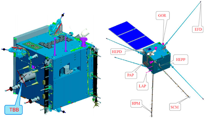
FIGURE 1. CSES-01 configuration {adapted from [Shen et al. (2018)]}.

The present study is based on EFD and SCM vector data within the geographical coordinate system. Following the approach reported in (Bertello et al., 2018), the analysis has focused on the ELF band (∼1 Hz to 2.2 kHz; sampling rate: 5 kHz) for the electric field, and on the ULF band (∼1 Hz–200 Hz; sampling rate: 1,024 Hz) for the magnetic field. Indeed, recent investigations [e.g., (Zong et al., 2022)]reveal that EM emissions associated with seismic activity are mainly found in the range from ∼50 to ∼300 Hz.

2.2 OMNI data

One of the purposes of this study is to assess the impact of solar activity on detection of anomalies. The solar forcing can be taken into account via geomagnetic indices, which are proxies of geomagnetic disturbances observed on ground. Geomagnetic conditions at mid/low latitudes are usually measured by the Disturbance storm time (Dst) and SYM-H indices [see, for example, (Lakhina and Tsurutani, 2016)]. They both are a measure of the symmetric ring-current intensity (Iyemori, 1990), but SYM-H is computed at higher time resolution (1 min) than Dst (1 h). In this work, SYM-H is employed to label days monitored for background calculation as quiet, disturbed, or storm. SYM-H data rely on the use of several magnetometer stations to calculate the symmetric portion of the horizontal component of the magnetic field near the equator [see (Wanliss and Showalter, 2006) for details]. Data used in this work are from the OMNI database (https://cdaweb.gsfc.nasa.gov/index.html, accessed on 23/01/2023), which represents one major data source for the space weather Community. OMNI is a multi-source compilation of solar wind data, interplanetary magnetic-field data, solar and geomagnetic indices, energetic particle fluxes (Papitashvili and King, 2006).

In the present study, SYM-H data span the period from 01 January 2019 to 30 September 2021 (1,004 days). An average SYM-H value is calculated for each day $(\overline{\mathrm{S}\mathrm{Y}\mathrm{M}-\mathrm{H}})$, and classified as follows:

$I_Q:\overline{\mathrm{S}\mathrm{Y}\mathrm{M}-\mathrm{H}}\in \left[-10\mathrm{n}\mathrm{T},10\mathrm{n}\mathrm{T}\right]$

$I_D:\overline{\mathrm{S}\mathrm{Y}\mathrm{M}-\mathrm{H}}\in \left[-40\mathrm{n}\mathrm{T},-10\mathrm{n}\mathrm{T}\right]$

$I_S:\mathrm{o}\mathrm{t}\mathrm{h}\mathrm{e}\mathrm{r}\mathrm{w}\mathrm{i}\mathrm{s}\mathrm{e}$

Where I_Q, I_D and I_S mark quiet, disturbed and stormy days, respectively.

Compared to what is commonly found in literature [e.g., (Bertello et al., 2018)], the selected intervals are much more stringent, which ensures that quiet days are effectively clear from any solar perturbation, and that disturbed days only include low-intensity solar disturbances. It is important to stress that slight variations in the bounds of any interval (±10 nT) do not significantly impact background evaluation, due to the effect of averaging over the entire cluster of days included in each interval.

For each of the two seismic areas under analysis, two background maps have been calculated, one representing the average ionospheric condition during quiet days, and the other describing the same average condition on disturbed days. No stormy background has been computed, due to challenging discrimination between internal and external drivers during a solar storm.

2.3 Non-stationary signal decomposition: The fast Iterative filtering

Time-frequency analysis has been performed in order to catch characteristic frequencies in EM signals measured by CSES-01. Since our observations are strongly non-stationary, the Fast Iterative Filtering (FIF) method has come in support for proper decomposition. FIF is a signal decomposition technique recently developed to accelerate its Iterative Filtering (IF) parent (Lin et al., 2009; Cicone and Zhou, 2017), which has proven stable and convergent in the management of non-stationary signals (Cicone, 2020).

Here, the three components of the electric/magnetic field f(t) are decomposed into “intrinsic mode components” (IMCs) according to the following equation:

$f\left(t\right)=\sum _{l=1}^{N}IM{C}_l\left(t\right)+r\left(t\right)(1)$

Where N is the number of the obtained IMCs, IMC_l(t) is the l-th IMC, and r(t) is the residue of the decomposition.

Figure 2 shows an example of FIF decomposition applied to electric field data, where the blue line represents the original signal, the red dashed line represents the baseline, and fluctuations (obtained by subtraction of the baseline from the original signal) are reported in black.

FIGURE 2

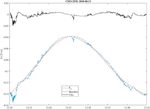
FIGURE 2. Application of the FIF technique to electric field data (expressed in V/m) from the CSES-01 satellite along an example orbit on 13 Aug 2018. The blue line represents the real signal, the red dashed line is the baseline, while fluctuations are shown in black.

Following the approach described in (Bertello et al., 2018) and (Piersanti et al., 2020b), the relation between each IMC and the l scale of variability for the f(t) signal is analyzed using the technique proposed in (Flandrin, 1998). Precisely, a signal marked by robust scale separation can be expressed as the sum of a baseline f₀t) and the variation δf(t) from the baseline:

$f\left(t\right)=f_0\left(t\right)+\delta f\left(t\right).(2)$

Here, δf(t) is identified by application of the method described by (Alberti et al., 2016):

$\delta f\left(t\right)=\sum _{l=1}^{k}IM{C}_l\left(t\right),(3)$

Where k is a subset of the N modes, and l is the scale of variability. In this way, it is possible to obtain a reconstruction of a subset of modes characterized by fluctuation at higher frequency and standardized mean SM ≈ 0 (SM being the mean divided by the standard deviation).

In this study, l represents the frequency of any IMC for either the electric or magnetic field.

2.4 The multiscale statistical analysis

In order to discern real signals from fluctuations of instrumental origin, we have performed multiscale statistical analysis. Specifically, at each frequency scale l we have calculated and studied the relative energy ϵ_rel

${ϵ}_{\mathit{rel}}\left(l,t\right)=\frac{{\int }_l|IM{C}_l\left(t\right){|}^{2}dt}{{\int }_l|f\left(t\right){|}^{2}dl},(4)$

Which represents the ratio of the energy corresponding to a specific time to the total energy over the whole time scale. The relative energy is then investigated as a function of the frequency and satellite latitude.

2.5 Background calculation

Both the environmental and instrumental backgrounds have been assessed.

The instrumental background has been evaluated by the technique described in Bertello et al.(2018).

For the environmental counterpart, we have considered all the orbits enclosed in a 6° × 6° geographic LAT-LON cell centered on the EE. For each of such orbits, we have performed the analysis described in Section 2.3 and Section 2.4.

All ϵ_rel values from calculation have been interpolated on a regular grid built as follows.

• for latitudes: a linear 0.1° spacing from ϕ_EE − 3° to ϕ_EE + 3° (ϕ_EE being the latitude of the EE).

• for frequencies: a logarithmic spacing ranging from $f_{\mathit{MIN}}^{\mathit{EFD}}\approx 1$ Hz to $f_{\mathit{MAX}}^{\mathit{EFD}}=2.2$ kHz for the electric field, and from $f_{\mathit{MIN}}^{\mathit{SCM}}\approx 1$ Hz to $f_{\mathit{MAX}}^{\mathit{SCM}}=200$ Hz for the magnetic field. The number of frequencies for the final grid is chosen as the average of the number of IMCs for each orbit.

In this way, a 60 × 17 (latitude × frequency) grid is obtained for EFD, and a 60 × 21 one for SCM, with ϵ_rel interpolated on every grid point. Starting from the set of the ϵ_rel spectra as a function of latitude and frequency, a background spectrum $(\overline{{ϵ}_{\mathit{rel}}})$ has been obtained as the mean value of ϵ_rel over the selected orbits.

For the sake of interpolation, CSES-01 orbits having a number of records less than 18 have been discarded, which amounts to discarding $\sim 10\%$ of the dataset. For each orbit, an additional selection criterion has been established in order to obtain a robust estimation of the average:

$\frac{{ϵ}_{\mathit{rel}}}{\overline{{ϵ}_{\mathit{rel}}}}\le 1\pm 5\frac{\sigma }{\overline{{ϵ}_{\mathit{rel}}}}(5)$

Where ϵ_rel is the relative energy (see Section 2.4), $\overline{{ϵ}_{\mathit{rel}}}$ is its mean value over all selected orbits, and σ is its standard deviation. Such a condition is complied with to ensure that possible anomalous orbits cannot contaminate the average.

Downstream of these selections and calculations, the obtained background ends up including only EM observations geographically close to the earthquake, and excluding outliers due to possible extreme events occurred before the seismic event.

The described procedure ensures that any signal statistically differing from the background is worthy of consideration as a possible event correlated to seismic activity.

A preliminary selection over quiet and disturbed days allows to obtain two corresponding backgrounds over any seismic region.

3 Case events

As mentioned earlier, the algorithm has been tested against two case events: the 14 August 2021 Haitian earthquake and the 27 September 2021 Cretan earthquake. Since marked by different geomagnetic conditions, it has been possible to assess the impact of solar activity on the analysis.

3.1 Case event: 14 August 2021–Haiti

On 14 August 2021, at 12:29:08 UTC, an earthquake struck the Tiburon Peninsula of Haiti, 150 km west of the capital Port-au-Prince. The magnitude of the event was 7.2 MW at EE geographical LAT-LON coordinates 18.417°N, 73.480°W (for details, see D’Angelo et al., 2022a and reference therein).

Following the procedure described in Section 2, we have computed the average backgrounds for quiet and disturbed geomagnetic conditions, which are shown in Figures 3, 4, respectively. In each of these figures, the ϵ_rel spectrum (color scale: ϵ_rel intensity) is reported as a function of frequency and satellite latitude. Panel a) shows the E_x (geographic north-south) component, panel b) shows the E_y (east-west) component, and panel c) the E_z (vertical) component.

FIGURE 3

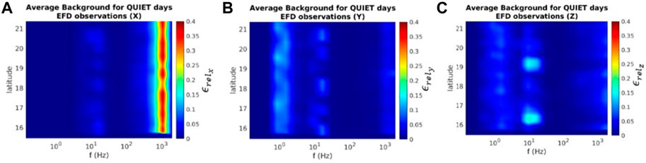
FIGURE 3. Average environmental background for quiet conditions for a 6° x 6° cell over Haiti, in terms of ϵ_rel intensity as a function of latitude and frequency for the three components of the electric field (E_x, E_y, E_z from left to right).

FIGURE 4

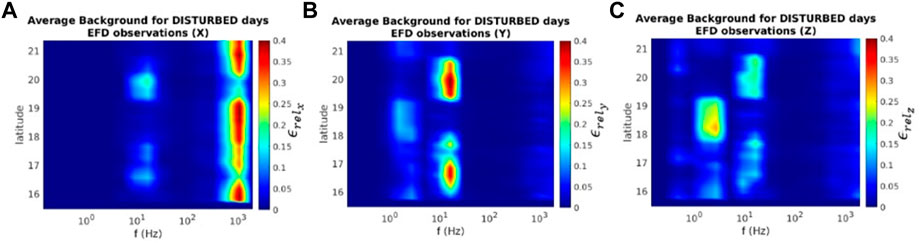
FIGURE 4. Average environmental background for disturbed conditions expressed as ϵ_rel intensity vs. latitude (depending on time) and frequency for the three components of the electric field. ϵ_rel values are generally larger than in the quiet case, but EM activity covers the same frequency bands.

By comparison of Figures 3, 4, it can be easily seen that “quiet” and “disturbed” spectra reveal activity in the same frequency bands, but at different energetic content (lower in the former case).

In particular, the following frequencies emerge from both spectra.

• ≈ 2 Hz (E_y, E_z): these peaks are due to the v × B electric field present in the ELF band, caused by satellite motion into the geomagnetic field [see e.g., (Diego et al., 2021)];

• ≈ 8 and ≈15 Hz (E_x, E_y, E_z): first and second Schumann ionospheric resonances at CSES-01 orbit [see (Rodríguez-Camacho et al., 2022)];

• ≈ 1 kHz (E_x): signature of the plasmaspheric hiss (Malaspina et al., 2018; Tsurutani et al., 2018).

Background spectra in Figures 3, 4 have been compared with the one obtained at the location of seismic activity, which is shown in Figure 5. For this event, CSES-01 was flying over the EE ∼6 h before the earthquake (Figure 6).

FIGURE 5

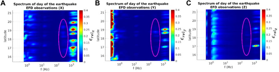
FIGURE 5. Spectra of 14 August 2021, 6 hours before the event, on the same 6° × 6° LAT-LON cell considered for background spectra. In addition to the ≈ 2 Hz and ≈ 1 kHz peaks present in background spectra, another signal can be detected at 250 ± 70 Hz (especially in the x and y components).

FIGURE 6

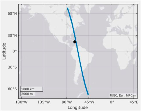
FIGURE 6. CSES-01 orbit (blue line) flying over the EE on 14 August 2021, 6 h before the earthquake. The black point represents the EE.

As it can be seen from Figure 7, the day when the EQ occurred was a disturbed one.

FIGURE 7

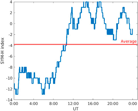
FIGURE 7. SYM-H index for 14 Aug 2021. Following the procedure described in Section 2.2, this day can be classified as disturbed, in spite of SYM-H going slightly below 10 nT for a few hours.

Comparing Figures 4, 5, signals at 2 Hz, 8 Hz, 15 Hz and 1 kHz appear in both sets. An additional signal at ∼250 ± 70 Hz (enclosed in magenta ellipses) appears in Figure 5 along the three components (more clearly in the x and y components).

The homologous analysis (Figure 8) has been repeated for the local magnetic field along the geographic North-South (B_x), East-West (B_y) and vertical (B_z) components. In this case, the $\overline{{ϵ}_{\mathit{rel,SCM}}}$ background spectra clearly show the signature of the second Schumann resonance at ∼16 Hz.

FIGURE 8

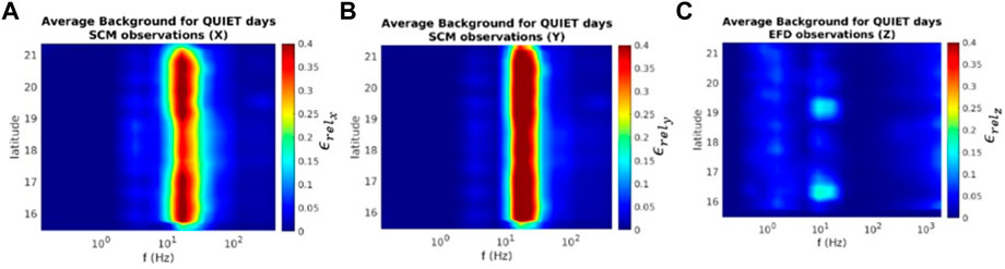
FIGURE 8. CSES-01/SCM observations. Environmental background evaluated in a 6° × 6° cell centered over the EE, in terms of $\overline{{ϵ}_{\mathit{rel}}}$ intensity vs latitude and frequency for disturbed conditions).

Figure 9 shows the relative energy of SCM observations on 14 August 2021, 6 hours before the earthquake. Again, the second Schumann resonance clearly appears in all components. An additional peak is detected in the same frequency band as already observed in EFD data ($\approx 190\pm 60$ Hz, enclosed in magenta ellipses), especially for the z component.

FIGURE 9

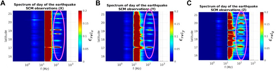
FIGURE 9. CSES-01/SCM observations on 14 August 2021, 6 hours before the event, when the satellite flew over the EE. In addition to the second Schumann resonance, another signal appears with more evidence in the z component.

3.2 Case event: 27 September 2021–Crete

A 6.0 M_W earthquake struck Crete (Greece) on 27 September 2021, at 06:17:22 UTC. The EE was located at (35.252°N, 25.260°E). The same analysis as the one reported in the preceding paragraph has been performed. The environmental background obtained under disturbed conditions is shown in Figure 10. CSES-01/EFD observations for 27 September 2021 appear in Figure 11. The satellite flew in the proximity of the EE about 17 h before the earthquake (Figure 12).

FIGURE 10

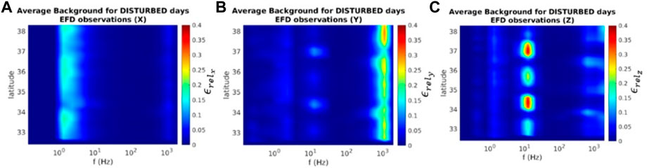
FIGURE 10. Average environmental background for disturbed conditions in a 6°x6° cell over the EE. The ionospheric signals already detected in the first case event can be found again.

FIGURE 11

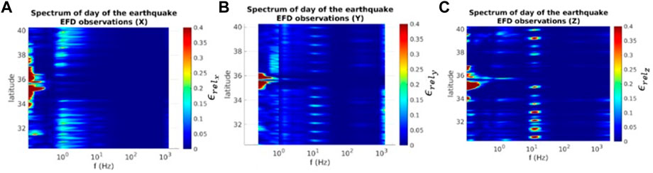
FIGURE 11. CSES-01/EFD spectra for 27 September 2021, 17 hours before the event, on the same 6° × 6° LAT-LON cell. In this case, no clear signal emerges from the background.

FIGURE 12

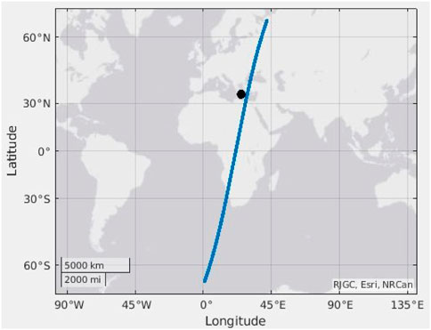
FIGURE 12. CSES-01 orbit (blue line) flying over the EE, 17 h before the earthquake. The black point represents the EE.

Once again, the background spectra include the ∼2 Hz signature due to satellite motion into the geomagnetic field, the Schumann resonance at ∼15 Hz, and the plasmaspheric hiss at ∼1 kHz. Quiet (not shown) and disturbed spectra show very similar behaviour.

Both Figures 10, 11 retain ionospheric signals at ∼2 Hz, ∼15 Hz and ∼1 kHz). Yet, a higher level of noise can be recovered in Figure 11 with respect to the seismic event in the first test, with no clear evidence of a definite signal standing out from the background. This is caused by dominant external (solar) forcing, as highlighted by the algorithm classifying the day as stormy (Figure 13).

FIGURE 13

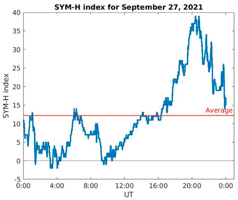
FIGURE 13. SYM-H index for September 27, 2021. This day is classified as stormy.

Same considerations hold for magnetic field observations (not shown).

In general, nothing significant emerges from the comparison between average background spectra and observations closely prior to EQ.

4 Discussion and conclusions

A proper identification of ionospheric and magnetospheric irregularities possibly connected to seismic activity has become an argument of great importance in space science research in the last few years, thanks to the increasing number of satellites in orbit and ground-based measurement facilities. In this scenario, a crucial role is represented by the accurate definition of a background for EM emissions over seismic regions, for the purposes of a precise and reliable detection of signals possibly induced by EQs.

The algorithm presented here represents a very efficient method to build an ionospheric background. Indeed, in order to exclude false positives and ensure a robust anomaly selection, it imposes a threshold on signal intensity (w. r. t. the background) equal to 5σ. In addition, it relies on the FIF technique, which represents the current state of the art for non-linear and non-stationary signal analysis (Ghobadi et al., 2020; Cicone and Pellegrino, 2022).

Also, it permits to take into account the impact of the solar driver on background determination. The magnetospheric and the ionospheric environments strongly depend on solar activity (Vellante et al., 2014; Piersanti et al., 2017). For this reason, the algorithm separately treats CSES-01 EM data for quiet, disturbed and stormy conditions. It is found that it is basically impossible to define an average spectrum during a geomagnetic storm (see Section 2.5), which is why two different backgrounds are calculated: one for orbits relative to quiet days and the other for disturbed days. In this way, a robust discrimination between external and internal drivers can be carried out.

Our procedure is able to correctly identify the characteristic frequencies of well known signals in the ionosphere, namely.

• the plasmaspheric hiss at ∼1 kHz (Malaspina et al., 2018; Tsurutani et al., 2018);

• the first and second Schumann resonance, at ∼8 and ∼15 Hz respectively (Rodríguez-Camacho et al., 2022);

• the signal due to the v × B field caused by the satellite motion into the geomagnetic field (Diego et al., 2021).

Also a ∼20 Hz signal in the magnetic field observations has been found (Figures 8, 9), which is the signature of the second Schumann resonance in the ELF portion of the Earth’s electromagnetic field, generated by lightning discharges in the cavity formed by the Earth’s surface and the ionosphere (Barr et al., 2000). Therefore, we can reasonably assert that the background obtained by our technique represents a first robust characterization of the top-side (∼500 km) ionospheric EM environment.

To test our algorithm during active seismic conditions, two case events have been investigated, namely the Haitian earthquake occurred on 14 August 2021 (under mildly disturbed geomagnetic conditions) and the Cretan earthquake occurred on 27 September 2021 (under stormy conditions). Possible EQ-related anomalies have been searched for by comparison of the EM energy spectrum evaluated around the EE (in a 6° × 6° LAT-LON cell) to the background, as closely as possible to the time of the seismic onset.

A summary of the two case events is shown in Table 1.

Haiti: The day is classified as disturbed, despite the SYM-H (see Figure 5) assumes values slightly below 10 nT (which is the value chosen as the limit between quiet and disturbed conditions) for a small time. Six hours before the earthquake occurrence, a ∼250 ± 70 Hz anomaly in the electric field and a ∼190 ± 60 Hz one in the magnetic field appear in energy spectra. No activities are found in disturbed background spectra at those frequencies, confirming that the signals are not usual ionospheric features. The two anomalies are perpendicular to each other. Since their frequencies are equal within uncertainties, it can be reasonably asserted that both of them identify an electromagnetic wave induced by seismic activity.

The clear detection of an electromagnetic wave possibly induced by an EQ and not related to solar forcing is an important experimental evidence. Ground motions induced by an earthquake in the ambient geomagnetic field, due to the conductivity of the Earth’s crust, can cause an electromotive force, which in turn leads to the rise of EM fields. In these last decades, this mechano-electric mechanism has been referred as the motional induction effect (Gershenzon et al., 1993; Yamazaki, 2012) or seismic dynamo effect (Matsushima et al., 2002), and it has been proposed as a possible explanation for the EM disturbances observed during large seismic events (Gershenzon and Bambakidis, 2001; Matsushima et al., 2002; Honkura et al., 2004; Ujihara et al., 2004; Yamazaki, 2012) mainly in the ionosphere (Pulinets and Boyarchuk, 2004). A promising formal framework to justify the coupling between lithosphere, atmosphere and ionosphere is given by the MILC model (Piersanti et al., 2020b; Carbone et al., 2021). This model assumes the generation of an acoustic gravity wave (AGW), which propagates through the atmosphere, and interacts with the ionosphere, also causing an EM wave injection into the Van Allen Belts.

The electromagnetic anomaly detected for the Haitian earthquake is well fitted by the model, representing an optimal example of litho/iono/magnetospheric coupling occurring during seismic activity (see (D’Angelo et al., 2022b)) and enlarging the range of experimental evidence compatible with MILC. Also, the frequency range of the anomalous signal is compatible with results showed in previous works (Piersanti et al., 2020b; Zong et al., 2022).

Crete: The day is classified as stormy. Despite the sensitivity of our technique, nothing clear emerges from the background close to the earthquake onset (Figures 10, 11). This is due to the high geomagnetic activity registered in the monitored day (Figure 13). Since the external forcing is dominant and the definition of a background spectra is pointless for stormy days, nothing can be concluded about the lithosphere-ionosphere-magnetosphere coupling in the case of the Cretan earthquake, and in general for seismic events accompanied by concurrent high geomagnetic activity. This case event highlights how essential a preliminary analysis of the geomagnetic conditions can be, and how challenging a neat separation between external and internal drivers can prove when high solar activity is at play.

TABLE 1

TABLE 1. Summary of the two investigated seismic events.

The analysis of the two case events reported in this study clearly shows that only a multi-disciplinary and multi-instrumental approach can lead to a reliable disentanglement of EQ-induced effects from changes due to other physical processes that govern the ionospheric dynamics.

With respect to previous studies (e.g., (Bertello et al., 2018), and reference therein), our work represents a step forward in the detection of electromagnetic anomalies possibly correlated to seismic activity, since several improvements have been added to the analysis. First of all, the construction of a grid with a logarithmic frequency scale (on which to remap all selected orbits) allows for a better comparison between observations and background, ensuring a better representation of the frequencies in the range of interest (around 100–200 Hz). Also, our method permits to better take into account the geomagnetic situation. Indeed, we have introduced the SYM-H index (1-min time resolution) and redefined thresholds in a more stringent way. This ensures that quiet days are in fact free from any solar disturbance, and that disturbed days only include low-intensity disturbances. Finally, the inclusion of 3 years of data (2019–2021) and the exclusion of outliers in the computation of the background leads to a robust estimation.

This work aims to reduce the lack of knowledge about lithosphere-ionosphere coupling. The proposed method could be used to compute the global background level (also reaching 1° × 1° spatial resolution) for comparison with in-flight CSES data, thus obtaining a global characterization of the ionosphere at satellite altitude. Furthermore, as already mentioned, CSES-01 payloads particle detectors as well. An improvement in the detection of EM anomalies could boost comparative analysis with particle flux enhancements possibly induced by seismic activity. Indeed, first evidences for mutual correlation between electron fluxes, EM emissions and large seismic events can be found in recent studies [e.g., (Anagnostopoulos et al., 2012)].

One last mention is the forthcoming launch of the CSES-02 satellite. The new element of the constellation will ensure a better coverage of the Earth’s seismic regions, and it will increase the probability of probe crossing in the proximity of the EE in a time window not far from EQ onset. This is expected to increase the effectiveness of the type of analysis presented here.

Data availability statement

CSES satellite data are freely available at the LEOS repository (www.leos.ac.cn, accessed on 11/11/2022); SYM-H data are freely available at the Cdaweb repository (https://cdaweb.gsfc.nasa.gov/index.html accessed on 23/01/2023).

Results can be reproduced using standard free analysis packages. Methods are fully described. Code used to produce figures can be made available upon request.

Author contributions

DR writing—Original draft preparation, formal analysis and methodology; GD’A writing—review and editing, formal analysis; EP writing—Review and editing; PD resources and data curation; AC methodology; AP writing—Review and editing; PU writing—Review and editing; RB writing—Review and editing, funding; MP. writing—Review and editing, supervision.

Acknowledgments

The authors kindly acknowledge N. Papitashvili and J. King at the National Space Science Data Center of the Goddard Space Flight Center for the use permission of 1-minute OMNI data and the NASA CDAWeb team for making these data available. The parameters of the 2021 Haitian earthquake are provided by USGS (https://earthquake.usgs.gov/200earthquakes/eventpage/us1000g3ub/executive) and INGV (http://terremoti.ingv.it/) datacatalogs. The authors thank the Italian Space Agency for the financial support under the contract ASI “LIMADOU Scienza+” n° 2020-31-HH.0. MPand GD’A thank the ISSI-BJ project “The electromagnetic data validation and scientific application research based on CSES satellite” and Dragon 5 cooperation 2020-2024 (ID. 59236).

Conflict of interest

The authors declare that the research was conducted in the absence of any commercial or financial relationships that could be construed as a potential conflict of interest.

Publisher’s note

All claims expressed in this article are solely those of the authors and do not necessarily represent those of their affiliated organizations, or those of the publisher, the editors and the reviewers. Any product that may be evaluated in this article, or claim that may be made by its manufacturer, is not guaranteed or endorsed by the publisher.

References

Alberti, T., Piersanti, M., Vecchio, A., De Michelis, P., Lepreti, F., Carbone, V., et al. (2016). Identification of the different magnetic field contributions during a geomagnetic storm in magnetospheric and ground observations. Ann. Geophys. 34, 1069–1084. doi:10.5194/angeo-34-1069-2016

CrossRef Full Text | Google Scholar

Anagnostopoulos, G. C., Vassiliadis, E., and Pulinets, S. (2012). Characteristics of flux-time profiles, temporal evolution, and spatial distribution of radiation-belt electron precipitation bursts in the upper ionosphere before great and giant earthquakes. Ann. Geophys. 55.

Google Scholar

Barr, R., Jones, D. L., and Rodger, C. (2000). Elf and vlf radio waves. J. Atmos. Solar-Terrestrial Phys. 62, 1689–1718. doi:10.1016/s1364-6826(00)00121-8

CrossRef Full Text | Google Scholar

Bertello, I., Piersanti, M., Candidi, M., Diego, P., and Ubertini, P. (2018). Electromagnetic field observations by the demeter satellite in connection with the 2009 l’aquila earthquake. Ann. Geophys. Copernic. GmbH) 36, 1483–1493. doi:10.5194/angeo-36-1483-2018

CrossRef Full Text | Google Scholar

Carbone, V., Piersanti, M., Materassi, M., Battiston, R., Lepreti, F., and Ubertini, P. (2021). A mathematical model of lithosphere–atmosphere coupling for seismic events. Sci. Rep. 11, 8682. doi:10.1038/s41598-021-88125-7

PubMed Abstract | CrossRef Full Text | Google Scholar

Cicone, A. (2020). Iterative filtering as a direct method for the decomposition of nonstationary signals. Numer. Algorithms 85, 811–827. doi:10.1007/s11075-019-00838-z

CrossRef Full Text | Google Scholar

Cicone, A., and Pellegrino, E. (2022). Multivariate fast iterative filtering for the decomposition of nonstationary signals. IEEE Trans. Signal Process. 70, 1521–1531. doi:10.1109/TSP.2022.3157482

CrossRef Full Text | Google Scholar

Cicone, A., and Zhou, H. (2017). Multidimensional iterative filtering method for the decomposition of high–dimensional non–stationary signals. Numer. Math. Theory, Methods Appl. 10, 278–298. doi:10.4208/nmtma.2017.s05

CrossRef Full Text | Google Scholar

Cicone, A., and Zhou, H. (2021). Numerical analysis for iterative filtering with new efficient implementations based on fft. Numer. Math. 147, 1–28. doi:10.1007/s00211-020-01165-5

CrossRef Full Text | Google Scholar

Cohen, M. B., and Inan, U. S. (2012). Terrestrial vlf transmitter injection into the magnetosphere. J. Geophys. Res. Space Phys. 117. doi:10.1029/2012JA017992

CrossRef Full Text | Google Scholar

D’Angelo, G., Piersanti, M., Battiston, R., Bertello, I., Carbone, V., Cicone, A., et al. (2022). Haiti earthquake (mw 7.2): Magnetospheric–ionospheric–lithospheric coupling during and after the main shock on 14 august 2021. Remote Sens. 14, 5340. doi:10.3390/rs14215340

CrossRef Full Text | Google Scholar

D’Angelo, G., Piersanti, M., Battiston, R., Bertello, I., Cicone, A., Diego, P., et al. (2022). “Investigation of the magnetospheric–ionospheric–lithospheric coupling on occasion of the 14 august 2021 haitian earthquake,” in Copernicus meetings. Tech. rep.

Google Scholar

Diego, P., Huang, J., Piersanti, M., Badoni, D., Zeren, Z., Yan, R., et al. (2021). The electric field detector on board the China seismo electromagnetic satellite—In-orbit results and validation. Instruments 5, 1. doi:10.3390/instruments5010001

CrossRef Full Text | Google Scholar

Flandrin, P. (1998). Time-frequency/time-scale analysis. Cambridge, Massachusetts: Academic Press.

Google Scholar

Gershenzon, N., and Bambakidis, G. (2001). Modeling of seismo-electromagnetic phenomena. Russ. J. Earth Sci. 3, 247–275. doi:10.2205/2001es000058

CrossRef Full Text | Google Scholar

Gershenzon, N. I., Gokhberg, M. B., and Yunga, S. (1993). On the electromagnetic field of an earthquake focus. Phys. earth Planet. interiors 77, 13–19. doi:10.1016/0031-9201(93)90030-d

CrossRef Full Text | Google Scholar

Ghobadi, H., Spogli, L., Alfonsi, L., Cesaroni, C., Cicone, A., Linty, N., et al. (2020). Disentangling ionospheric refraction and diffraction effects in gnss raw phase through fast iterative filtering technique. GPS Solutions 24, 85. doi:10.1007/s10291-020-01001-1

CrossRef Full Text | Google Scholar

Hayakawa, M., Kasahara, Y., Nakamura, T., Hobara, Y., Rozhnoi, A., Solovieva, M., et al. (2011). Atmospheric gravity waves as a possible candidate for seismo-ionospheric perturbations. J. Atmos. Electr. 31, 129–140. doi:10.1541/jae.31.129

CrossRef Full Text | Google Scholar

Hayakawa, M. (2015). Earthquake prediction with radio techniques. Hoboken, New Jersey: John Wiley & Sons. doi:10.1002/9781118770368

CrossRef Full Text | Google Scholar

Hines, C. O. (1960). Internal atmospheric gravity waves at ionospheric heights. Can. J. Phys. 38, 1441–1481. doi:10.1139/p60-150

CrossRef Full Text | Google Scholar

Honkura, Y., Satoh, H., and Ujihara, N. (2004). Seismic dynamo effects associated with the m7. 1 earthquake of 26 may 2003 off miyagi prefecture and the m6. 4 earthquake of 26 july 2003 in northern miyagi prefecture, ne Japan. Earth, planets space 56, 109–114. doi:10.1186/bf03353395

CrossRef Full Text | Google Scholar

Iyemori, T. (1990). Storm-time magnetospheric currents inferred from mid-latitude geomagnetic field variations. J. geomagnetism Geoelectr. 42, 1249–1265. doi:10.5636/jgg.42.1249

CrossRef Full Text | Google Scholar

Lagoutte, D., Brochot, J., de Carvalho, D., Elie, F., Harivelo, F., Hobara, Y., et al. (2006). The demeter science mission centre. Planet. Space Sci. 54, 428–440. First Results of the DEMETER Micro-Satellite. doi:10.1016/j.pss.2005.10.014

CrossRef Full Text | Google Scholar

Lakhina, G. S., and Tsurutani, B. T. (2016). Geomagnetic storms: Historical perspective to modern view. Geosci. Lett. 3, 5–11. doi:10.1186/s40562-016-0037-4

CrossRef Full Text | Google Scholar

Lin, L., Wang, Y., and Zhou, H. (2009). Iterative filtering as an alternative algorithm for empirical mode decomposition. Adv. Adapt. Data Analysis 1, 543–560. doi:10.1142/s179353690900028x

CrossRef Full Text | Google Scholar

Malaspina, D. M., Ripoll, J. F., Chu, X., Hospodarsky, G., and Wygant, J. (2018). Variation in plasmaspheric hiss wave power with plasma density. Geophys. Res. Lett. 45, 9417–9426. doi:10.1029/2018gl078564

CrossRef Full Text | Google Scholar

Matsushima, M., Honkura, Y., Oshiman, N., Baris, S., Tunçer, M., Tank, S., et al. (2002). Seismoelectromagnetic effect associated with the izmit earthquake and its aftershocks. Bull. Seismol. Soc. Am. 92, 350–360. doi:10.1785/0120000807

CrossRef Full Text | Google Scholar

Mikumo, T., and Watada, S. (2010). “Acoustic-gravity waves from earthquake sources,” in Infrasound Monitoring for Atmospheric Studies. Editors A. Le Pichon, E. Blanc, and A. Hauchecorne (Dordrecht: Springer). doi:10.1007/978-1-4020-9508-5_9

CrossRef Full Text | Google Scholar

Miyaki, K., Hayakawa, M., and Molchanov, O. (2002). The role of gravity waves in the lithosphere-ionosphere coupling, as revealed from the subionospheric lf propagation data. Seismo Electromagn. Lithosphere-Atmosphere-Ionosphere Coupling, 229–232.

Google Scholar

Molchanov, O., Hayakawa, M., and Miyaki, K. (2001). Vlf/lf sounding of the lower ionosphere to study the role of atmospheric oscillations in the lithosphere-ionosphere coupling. Advances in polar upper atmosphere research 15, 146–158.

Google Scholar

Molchanov, O. A., and Hayakawa, M. (1998). Subionospheric vlf signal perturbations possibly related to earthquakes. J. Geophys. Res. Space Phys. 103, 17489–17504. doi:10.1029/98JA00999

CrossRef Full Text | Google Scholar

Muto, F., Kasahara, Y., Hobara, Y., Hayakawa, M., Rozhnoi, A., Solovieva, M., et al. (2009). Further study on the role of atmospheric gravity waves on the seismo-ionospheric perturbations as detected by subionospheric vlf/lf propagation. Nat. Hazards Earth Syst. Sci. 9, 1111–1118. doi:10.5194/nhess-9-1111-2009

CrossRef Full Text | Google Scholar

Němec, F., Santolík, O., and Parrot, M. (2009). Decrease of intensity of elf/vlf waves observed in the upper ionosphere close to earthquakes: A statistical study. J. Geophys. Res. Space Phys. 114. doi:10.1029/2008JA013972

CrossRef Full Text | Google Scholar

Papitashvili, N., and King, J. (2006). “A draft high resolution omni data set,” in AGU spring meeting abstracts, 2007, SM33A–02.

Google Scholar

Piersanti, M., Alberti, T., Bemporad, A., Berrilli, F., Bruno, R., Capparelli, V., et al. (2017). Comprehensive analysis of the geoeffective solar event of 21 june 2015: Effects on the magnetosphere, plasmasphere, and ionosphere systems. Sol. Phys. 292. doi:10.1007/s11207-017-1186-0

CrossRef Full Text | Google Scholar

Piersanti, M., De Michelis, P., Del Moro, D., Tozzi, R., Pezzopane, M., Consolini, G., et al. (2020). From the sun to Earth: Effects of the 25 august 2018 geomagnetic storm. Ann. Geophys. 38, 703–724. doi:10.5194/angeo-38-703-2020

CrossRef Full Text | Google Scholar

Piersanti, M., Materassi, M., Battiston, R., Carbone, V., Cicone, A., D’Angelo, G., et al. (2020). Magnetospheric–ionospheric–lithospheric coupling model. 1: Observations during the 5 august 2018 bayan earthquake. Remote Sens. 12, 3299. doi:10.3390/rs12203299

CrossRef Full Text | Google Scholar

Pulinets, S., and Boyarchuk, K. (2004). Ionospheric precursors of earthquakes. Berlin, Germany: Springer Science & Business Media.

Google Scholar

Pulinets, S., Ouzounov, D., Karelin, A., and Boyarchuk, K. (2022). Multiparameter approach and LAIC validation. Dordrecht: Springer Netherlands, 187–247. doi:10.1007/978-94-024-2172-9_4

CrossRef Full Text | Google Scholar

Rodríguez-Camacho, J., Salinas, A., Carrión, M. C., Portí, J., Fornieles-Callejón, J., and Toledo-Redondo, S. (2022). Four year study of the schumann resonance regular variations using the sierra Nevada station ground-based magnetometers. J. Geophys. Res. Atmos. 127, e2021JD036051. doi:10.1029/2021JD036051.E2021JD0360512021JD036051

CrossRef Full Text | Google Scholar

Shen, X., Zhang, X., Yuan, S., Wang, L., Cao, J., Huang, J., et al. (2018). The state-of-the-art of the China seismo-electromagnetic satellite mission. Sci. China Technol. Sci. 61, 634–642. doi:10.1007/s11431-018-9242-0

CrossRef Full Text | Google Scholar

Tsurutani, B. T., Park, S. A., Falkowski, B. J., Lakhina, G. S., Pickett, J. S., Bortnik, J., et al. (2018). Plasmaspheric hiss: Coherent and intense. J. Geophys. Res. Space Phys. 123. doi:10.1029/2018ja025975

CrossRef Full Text | Google Scholar

Ujihara, N., Honkura, Y., and Ogawa, Y. (2004). Electric and magnetic field variations arising from the seismic dynamo effect for aftershocks of the m7. 1 earthquake of 26 may 2003 off miyagi prefecture, ne Japan. Earth, planets space 56, 115–123. doi:10.1186/bf03353396

CrossRef Full Text | Google Scholar

Vellante, M., Piersanti, M., and Pietropaolo, E. (2014). Comparison of equatorial plasma mass densities deduced from field line resonances observed at ground for dipole and igrf models. J. Geophys. Res. Space Phys. 119, 2623–2633. doi:10.1002/2013ja019568

CrossRef Full Text | Google Scholar

Villante, U., and Piersanti, M. (2011). Sudden impulses at geosynchronous orbit and at ground. J. Atmos. Solar-Terrestrial Phys. 73, 61–76. doi:10.1016/j.jastp.2010.01.008

CrossRef Full Text | Google Scholar

Walker, S. N., Kadirkamanathan, V., and Pokhotelov, O. A. (2013). Changes in the ultra-low frequency wave field during the precursor phase to the sichuan earthquake: Demeter observations. Ann. Geophys. 31, 1597–1603. doi:10.5194/angeo-31-1597-2013

CrossRef Full Text | Google Scholar

Wang, Q., Huang, J., Zhao, S., Zhima, Z., Yan, R., Lin, J., et al. (2022). The electromagnetic anomalies recorded by cses during yangbi and madoi earthquakes occurred in late may 2021 in west China. Nat. Hazards Res. 2, 1–10. doi:10.1016/j.nhres.2022.01.003

CrossRef Full Text | Google Scholar

Wanliss, J. A., and Showalter, K. M. (2006). High-resolution global storm index: Dst versus sym-h. J. Geophys. Res. Space Phys. 111, A02202. doi:10.1029/2005JA011034

CrossRef Full Text | Google Scholar

Yamazaki, K. (2012). Estimation of temporal variations in the magnetic field arising from the motional induction that accompanies seismic waves at a large distance from the epicentre. Geophys. J. Int. 190, 1393–1403. doi:10.1111/j.1365-246x.2012.05586.x

CrossRef Full Text | Google Scholar

Zong, J., Tao, D., and Shen, X. (2022). Possible elf/vlf electric field disturbances detected by satellite cses before major earthquakes. Atmosphere 13, 1394. doi:10.3390/atmos13091394

CrossRef Full Text | Google Scholar

Zhang, X., Fidani, C., Huang, J., Shen, X., Zeren, Z., and Qian, J. (2013). Burst increases of precipitating electrons recorded by the demeter satellite before strong earthquakes. Nat. Hazards Earth Syst. Sci. 13, 197–209. doi:10.5194/nhess-13-197-2013

CrossRef Full Text | Google Scholar

Zhang, X., Shen, X., Parrot, M., Zeren, Z., Ouyang, X., Liu, J., et al. (2012). Phenomena of electrostatic perturbations before strong earthquakes (2005–2010) observed on demeter. Nat. Hazards Earth Syst. Sci. 12, 75–83. doi:10.5194/nhess-12-75-2012

CrossRef Full Text | Google Scholar

Zhao, S., Zhou, C., Shen, X., and Zhima, Z. (2019). Investigation of vlf transmitter signals in the ionosphere by zh-1 observations and full-wave simulation. J. Geophys. Res. Space Phys. 124, 4697–4709. doi:10.1029/2019JA026593

CrossRef Full Text | Google Scholar

Zhima, Z., Hu, Y., Piersanti, M., Shen, X., De Santis, A., Yan, R., et al. (2020). The seismic electromagnetic emissions during the 2010 mw 7.8 northern sumatra earthquake revealed by demeter satellite. Front. Earth Sci. 8. doi:10.3389/feart.2020.572393

CrossRef Full Text | Google Scholar