An efficient spectral element method for two-dimensional magnetotelluric modeling

1 Introduction

As a special geo-electromagnetic method, magnetotelluric sounding can identify the resistivity or conductivity distributions in a geological medium based on harmonic and variable electromagnetic fields (Chave and Jones, 2012). Magnetotelluric sounding is based on naturally occurring electromagnetic fields, which can provide a comprehensive and continuous spectrum of the geo-electromagnetic field. This electrical resistivity, measured by comparing the electric field’s horizontal component to the magnetic field on the surface, can detect a depth of several tens of kilometers associated with the acquisition frequency. With the rapid advancement in magnetotelluric modeling and inversion, it has become one of the essential tools for recognizing deep geological structures (Unsworth, 2010; Avdeeva et al., 2012; Azeez et al., 2017; Nagarjuna et al., 2021) and geophysical investigations, such as geothermal exploration (Barcelona et al., 2013; Patro, 2017; Tarek et al., 2023), mineral deposit exploration (Benjamin et al., 2018; Jiang et al., 2022), and gas exploration (Zhang et al., 2014).

There are some numerical approaches for solving two-dimensional magnetotelluric forward problems, such as finite difference and finite element, and they are applied to two-dimensional magnetotelluric inversion (deGroot-Hedlin and Constable, 1990; Rodi and Mackie, 2001; Siripunvaraporn and Egbert, 2007; Lee et al., 2009; Kelbert et al., 2014; Guo et al., 2020; Liao et al., 2022). The finite difference numerical approach can solve partial differential equations for approximating first-order or second-order derivatives with a difference scheme (Pek and Verner, 1997; deGroot-Hedlin, 2006; Rao and Babu, 2006; Kumar et al., 2011). They also investigated the efficiency of computing two-dimensional magnetotelluric responses. This method also has high accuracy on the electric field and magnetic field components (Guo et al., 2018; Kalscheuer et al., 2018; Sarakorn and Vachiratienchai, 2018). Unfortunately, it is not easy to compute the resulting fields’ accurate apparent resistivities and phases. As another important numerical approach, finite element can be applied to solve the two-dimensional magnetotelluric forward problem (Wannamaker et al., 1986; Key and Weiss, 2006; Franke et al., 2007; Lee et al., 2009; Sarakorn, 2017; Yao et al., 2021). It involves the hypothetical functional form of the model and the field in a small area of the specified geometry. The finite element method can introduce complex information from the real world to construct the initial model, including surface topography, and can also improve the flexibility of mesh discretization. However, it requires fine meshing to obtain high accuracy, which results in high computational costs. Some other numerical methods are also used to simulate two-dimensional magnetotelluric forward modeling, such as the boundary element (Xu and Zhou, 1997), the finite-volume (Du et al., 2016; Wang et al., 2019), the mesh-free (Wittke and Tezkan, 2014; Wittke and Tezkan, 2021), the domain decomposition (Bihlo et al., 2017), the numerical manifold (Liang et al., 2021), and the pseudo-spectral methods (Tong et al., 2020). These numerical methods provide an essential practical basis for two-dimensional magnetotelluric forward modeling.

Compared to other numerical approaches, the finite element method requires fine grids to obtain higher calculation accuracy. This will bring challenges, especially when computational resources are limited. Moreover, in practical geophysical applications, when the discrete meshes need be refined to a geo-electrical model, the convergence rate will decrease gradually, while the number of meshes and the computational cost can increase largely (Key and Weiss, 2006). The spectral method, as a novel approach, can provide the numerical approximation of partial differential equations (Zou and Cheng, 2018). In this numerical approach, the field in the computational domain can be approximated by polynomials or Fourier expansions. Since high-order orthogonal basis functions are applied in the spectral method, it has exponential convergence. In addition, the spectral interpolation points are densely distributed at the boundary, which can avoid the Runge phenomenon in the traditional high-order interpolation (Tong et al., 2020). The method that combines the finite element and spectral method is called the spectral element method. In the past 20 years, geophysicists have dedicated these numerical methods to developing efficiency and accuracy. Some recent developments found that the spectral element approach can be seen as a high-order finite element method and its high-accuracy is derived from the properties of the spectral method (Patera, 1984). It can combine the high-accuracy of the spectral method and the flexibility of the finite element technique. Compared with the classical finite element method, the Runge phenomenon of isometric interpolation can be avoided using Gaussian orthogonal basis functions and Gaussian points (Xu et al., 2022). There are two types of spectral element methods, one based on Legendre polynomials and another based on Chebyshev polynomials. It is widely used in applications for wave propagation (Komatitsch and Tromp, 1999; Seriani and Oliveria, 2008; Luo et al., 2013; Trinh et al., 2019; Lyu et al., 2020), forward gravity modeling (Ghariti et al., 2018; Martin et al., 2017), and for geo-electromagnetic forward modeling problems (Zhou et al., 2016; Huang et al., 2019; Yin et al., 2019; Zhu et al., 2020; Huang et al., 2021; Weiss et al., 2023). However, it is rarely used in two-dimensional magnetotelluric forward modeling.

This paper proposes an efficient and accurate spectral element approach to compute the two-dimensional magnetotelluric responses of the boundary problem without measuring Earth’s curvature. To benchmark the accuracy, we compare the numerical results of the spectral element forward algorithm with the analytical solutions and numerical results of the finite difference and finite element schemes. Although our approach can be applied to any two-dimensional geo-electromagnetic forward modeling, in this study, we demonstrate its implementation mainly in numerical experiments.

2 Boundary value problem

2.1 Electromagnetic equations

We define the z-axis at the depth and the x-axis along the geologic strike, as shown in Figure 1. Using a time-harmonic factor $e^{-i\omega t}$, Maxwell’s equations can then be written as (Wannamaker et al., 1987; Yao et al., 2021)

$\nabla \times \mathit{E}=i\omega \mu \mathit{H}(1)$

$\nabla \times \mathit{H}=\sigma \mathit{E}(2)$

where E means the electric field, H represents the magnetic field, $\omega$ denotes the angular frequency, $\mu =4\pi \times {10}^{-7}\mathrm{H}/\mathrm{m}$ is the magnetic permeability, and $\sigma$ is the conductivity.

FIGURE 1

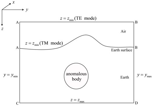
FIGURE 1. Geo-electrical model of the two-dimensional magnetotelluric forward problem.

For a two-dimensional structure, due to $\partial \mathit{E}/\partial x\equiv 0$ and $\partial \mathit{H}/\partial x\equiv 0$, we can expand the curl operators in Eqs 1, 2as follows:

$\frac{\partial E_z}{\partial y}-\frac{\partial E_y}{\partial z}=i\omega \mu H_x(3)$

$\frac{\partial E_x}{\partial z}=i\omega \mu H_y(4)$

$\frac{\partial E_x}{\partial y}=-i\omega \mu H_z(5)$

and

$\frac{\partial H_z}{\partial y}-\frac{\partial H_y}{\partial z}=\sigma E_x(6)$

$\frac{\partial H_x}{\partial z}=\sigma E_y(7)$

$\frac{\partial H_x}{\partial y}=-\sigma E_z(8)$

The electromagnetic equations are more complex than homogeneous media for two-dimensional modeling, where resistivity changes occur in the y-axis and z-axis. According to Eqs 4–6, $E_x$ the TE mode can yield a second-order Helmholtz equation:

$\frac{{\partial }^2{E}_x}{\partial y^2}+\frac{{\partial }^2{E}_x}{\partial z^2}+i\omega \mu \sigma E_x=0(9)$

Meanwhile, for the TM mode, $H_x$ yields another second-order Helmholtz equation:

$\frac{\partial }{\partial y}\left(\frac{1}{\sigma }\frac{\partial H_x}{\partial y}\right)+\frac{\partial }{\partial z}\left(\frac{1}{\sigma }\frac{\partial H_x}{\partial z}\right)+i\omega \mu H_x=0(10)$

Then the electric field $E_x$ or the magnetic field $H_x$ in the Helmholtz-type equation can be rewritten as

$\nabla \cdot \left(\tau \nabla u\right)+\lambda u=0(11)$

where u, $\tau$, and $\lambda$ represent different meanings relying on the different polarized modes. In the TE mode,

$u=E_x,\tau =\frac{1}{i\omega \mu },\lambda =\sigma (12)$

and in the TM mode,

$u=H_x,\tau =\frac{1}{\sigma },\lambda =i\omega \mu (13)$

2.2 Boundary conditions

We restrict the computational region for Eq. 11 to a two-dimensional bounded domain $\mathrm{\Omega }=\left[y_{\min },y_{\max }\right]\times \left[z_{\min },z_{\max }\right]$, as shown in Figure 1. Therefore, the boundary conditions in the computational domain can be expressed as

${\left.u\right|}_{z=z_{\min }}=1\left(\mathrm{i}\mathrm{n}\mathrm{A}\mathrm{B}\right)(\mathrm{14a})$

${\left.\frac{\partial u}{\partial y}\right|}_{y=y_{\min }}=0\left(\mathrm{i}\mathrm{n}\mathrm{A}\mathrm{C}\right),{\left.\frac{\partial u}{\partial y}\right|}_{y=y_{\max }}=0\left(\mathrm{i}\mathrm{n}\mathrm{B}\mathrm{D}\right)(\mathrm{14b})$

${\left.\left(\frac{\partial u}{\partial z}+ku\right)\right|}_{z=z_{\max }}=0\left(\mathrm{i}\mathrm{n}\mathrm{C}\mathrm{D}\right)(\mathrm{14c})$

where $k=\sqrt{-i\omega \mu \sigma }$.

3 Spectral element formulation

3.1 Discretization of a variational problem

The magnetotelluric fields can be simulated by the Helmholtz equation of Eq. 12 under the boundary conditions of Eq. 14. Using the variational principle (Pozrikidis, 2014), the boundary value problem of the partial differential form displayed in Eq. 12 and Eq. 14 can be written as the variational problem of the integral form:

$\left\{\begin{array}{l}F\left(u\right)=\iint \left\{\frac{1}{2}\tau \left[{\left(\frac{\partial u}{\partial y}\right)}^2+{\left(\frac{\partial u}{\partial z}\right)}^2\right]-\frac{1}{2}\lambda u^2\right\}\mathrm{d}y\mathrm{d}z+{\int }_{CD}\frac{1}{2}\tau k{u}^2\mathrm{d}l=\min \\ {\left.u\right|}_{y=y_{\min }}=0.\end{array}\right.(15)$

Within spectral element approximation, the magnetotelluric field can be expanded with two-dimensional interpolation basis functions:

$\mathit{u}={\displaystyle \sum _{i=1}^{N_r}}{N}_i\left(\xi ,\eta \right)u_i(16)$

where $N_r$ is the number of primary procedures for an element and $N_i\left(\xi ,\eta \right)$ are the essential functions.

The integral of all elements, Eq. 15, can be rewritten as

$F\left(u\right)=\sum {{\displaystyle \iint }}_e\left\{\frac{1}{2}\tau \left[{\left(\frac{\partial u}{\partial y}\right)}^2+{\left(\frac{\partial u}{\partial z}\right)}^2\right]-\frac{1}{2}\lambda u^2\right\}\mathrm{d}y\mathrm{d}z+\sum {{\displaystyle \int }}_{CD}\frac{1}{2}\tau k{u}^2\mathrm{d}l=\min (17)$

This will lead to a discrete linear equation as follows:

$\mathit{K}\mathit{u}=0(18)$

where u represents the values of the unknown magnetic field or electric field.

3.2 Spectral basis functions

Its spectral accuracy characterizes the spectral element, i.e., the numerical error depends on the order of the basis functions (Lee and Liu, 2005). We choose Gauss–Lobatto–Legendre (GLL) element discretization for the magnetotelluric forward problem. The Nth-order GLL basis functions in a one-dimensional reference element $\xi \in \left[-\mathrm{1,1}\right]$ can be expressed by

${\varphi }_i\left(\xi \right)=\frac{1}{N\left(N+1\right)L_N\left({\xi }_i\right)}\frac{{\xi }^2-1}{\xi -{\xi }_i}{L}_N^{\prime }\left(\xi \right)(19)$

for $i=\mathrm{1,2},\cdots ,N+1$, where $L_N\left(\xi \right)$ is the Nth-order Legendre polynomial and $L_N^{\prime }\left(\xi \right)$ is its derivative. On a reference element with $\xi ,\eta \in \left[-\mathrm{1,1}\right]\times \left[-\mathrm{1,1}\right]$, the two-dimensional basis function can be written as

$N_{ij}\left(\xi ,\eta \right)={\varphi }_i\left(\xi \right){\varphi }_j\left(\eta \right)(20)$

For example, if order p = 4, there are 25 basis functions to the interpolation nodes. Figure 2 shows two-dimensional basis functions of the 4th order in part, and four of the nodal basis functions corresponding to $N_{12}\left(\xi ,\eta \right)={\varphi }_1\left(\xi \right){\varphi }_2\left(\eta \right)$, $N_{22}\left(\xi ,\eta \right)={\varphi }_2\left(\xi \right){\varphi }_2\left(\eta \right)$, $N_{34}\left(\xi ,\eta \right)={\varphi }_3\left(\xi \right){\varphi }_4\left(\eta \right)$, and $N_{45}\left(\xi ,\eta \right)={\varphi }_4\left(\xi \right){\varphi }_5\left(\eta \right)$ are represented.

FIGURE 2

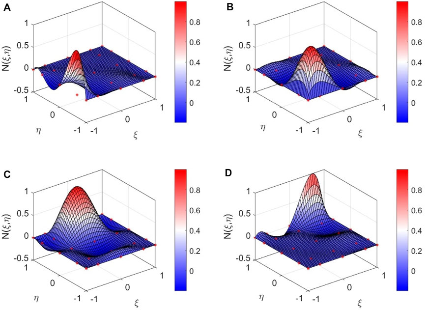
FIGURE 2. Two-dimensional spectral basis functions in part of order p=4. (A) $N_{12}\left(\xi ,\eta \right)={\varphi }_1\left(\xi \right){\varphi }_2\left(\eta \right)$; (B) $N_{22}\left(\xi ,\eta \right)={\varphi }_2\left(\xi \right){\varphi }_2\left(\eta \right)$; (C) $N_{34}\left(\xi ,\eta \right)={\varphi }_3\left(\xi \right){\varphi }_4\left(\eta \right)$; and (D) $N_{45}\left(\xi ,\eta \right)={\varphi }_4\left(\xi \right){\varphi }_5\left(\eta \right)$.

3.3 Spectral element equation

In the spectral element method, a physical sub-element needs to be mapped into a reference parent element and the element coefficient matrix can be achieved in the reference element. Figure 3 shows a mapping example of a two-dimensional spectral element $\left(y,z\right)$-coordinate and the normalized $\xi ,\eta \in \left[-\mathrm{1,1}\right]\times \left[-\mathrm{1,1}\right]$ reference coordinate.

FIGURE 3

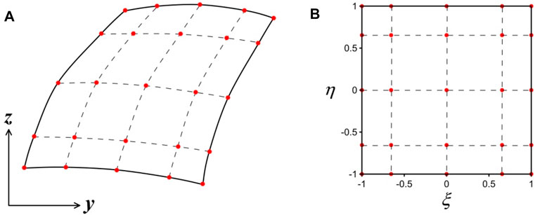
FIGURE 3. Mapping coordinate system of the spectral element of order p = 4. (A) Sub-element; (B) parent element.

The derivatives and the volume in the $\left(y,z\right)$-coordinate system in Eq. 17 can be transformed to the $\left(\xi ,\eta \right)$-coordinate system as follows:

$\mathrm{d}y\mathrm{d}z=\left|\begin{array}{l}\frac{\partial y}{\partial \xi }\frac{\partial z}{\partial \xi }\\ \frac{\partial y}{\partial \eta }\frac{\partial z}{\partial \eta }\end{array}\right|\mathrm{d}\xi \mathrm{d}\eta =\left|J\right|\mathrm{d}\xi \mathrm{d}\eta (21)$

where J is the Jacobian matrix.

The first-term integral in Eq. 17 is

${\iint }_e\frac{1}{2}\tau \left[{\left(\frac{\partial u}{\partial y}\right)}^2+{\left(\frac{\partial u}{\partial z}\right)}^2\right]\mathrm{d}y\mathrm{d}z=\frac{1}{2}{\mathit{u}}_e^T{\mathit{K}}_{1\mathit{e}}{\mathit{u}}_e(22)$

where

$\begin{array}{l}{\mathit{K}}_{1\mathit{e}}={\iint }_e\left[{\left(\frac{\partial u}{\partial y}\right)}^2+{\left(\frac{\partial u}{\partial z}\right)}^2\right]\mathrm{d}y\mathrm{d}z\\ ={\int }_{-1}^1{\int }_{-1}^1\tau \left(\frac{\partial N_i}{\partial \xi }\frac{\partial \xi }{\mathrm{d}y}\right)\left(\frac{\partial N_j}{\partial \xi }\frac{\partial \xi }{\partial y}\right)\left|J\right|\mathrm{d}\xi \mathrm{d}\eta +{\int }_{-1}^1{\int }_{-1}^1\tau \left(\frac{\partial N_i}{\partial \eta }\frac{\partial \eta }{\partial z}\right)\left(\frac{\partial N_j}{\partial \eta }\frac{\partial \eta }{\partial z}\right)\left|J\right|\mathrm{d}\xi \mathrm{d}\eta \end{array}$

The second-term integral in Eq. 17 is

${\iint }_e\frac{1}{2}\lambda u^2\mathrm{d}y\mathrm{d}z=\frac{1}{2}{\mathit{u}}_e^T{\mathit{K}}_{2\mathit{e}}{\mathit{u}}_e(23)$

where ${\mathit{K}}_{2\mathit{e}}={\iint }_e\lambda u^2\mathrm{d}y\mathrm{d}z={\int }_{-1}^1{\int }_{-1}^1\lambda N_i{N}_j\left|J\right|\mathrm{d}\xi \mathrm{d}\eta$.

The third-term integral in Eq. 17 is

${\int }_{CD}\frac{1}{2}\tau k{u}^2\mathrm{d}l=\frac{1}{2}{\mathit{u}}_e^T{\mathit{K}}_{3\mathit{e}}{\mathit{u}}_e(24)$

where ${\mathit{K}}_{3\mathit{e}}$ can be obtained with a one-dimensional line integral.

Considering the Dirichlet boundary condition at $z=z_{\min }$, we can derive the linear equations with the spectral element approach to build the two-dimensional magnetotelluric forward modeling:

$\mathit{K}\mathit{u}=\mathit{p}(25)$

where $\mathit{K}={\displaystyle \sum _{i=1}^{N_e}}{\mathit{K}}_{1\mathit{e}}-{\displaystyle \sum _{i=1}^{N_e}}{\mathit{K}}_{2\mathit{e}}+{\displaystyle \sum _{i=1}^{N_e}}{\mathit{K}}_{3\mathit{e}}$ is the coefficient matrix containing conductivity parameters $\sigma$, and $N_e$ is the number of all elements. The right-side vector p is interrelated to the Dirichlet boundary conditions. The coefficient matrix K is a sparse, positive-defined, symmetric matrix. Figure 4 shows the sparse elements’ distribution of the coefficient matrix for a 3 × 3 grid with the 4th polynomial order (just for illustration purposes). We use the biconjugate gradient-stabilized algorithm (van der Vorst, 1992; Chen et al., 2002), preconditioned with incomplete LU factorization (Pan et al., 2022), for our forward problem.

FIGURE 4

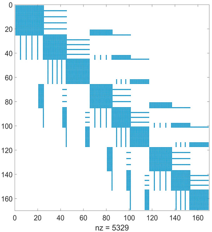
FIGURE 4. Non-zero sparse elements of the discretization coefficient matrix obtained a 3 × 3 grid with a fourth-order polynomial spectral element approach.

After obtaining $E_x$, the corresponding magnetic field component $H_y$ can be solved by Eq. 4 for the TE mode. Since we acquired $H_x$, the corresponding electric component $E_y$ can be solved by Eq. 7 for the TM mode. Then, we can obtain the two-dimensional impedance tensor from

$\left[\begin{array}{l}{E}_x\\ E_y\end{array}\right]=\left[\begin{array}{l}0Z_{xy}\\ Z_{yx}0\end{array}\right]\left[\begin{array}{l}{H}_x\\ H_y\end{array}\right](26)$

The impedance can be used to calculate apparent resistivities

${\rho }_a^{xy}=\frac{1}{\omega \mu }{\left|Z_{xy}\right|}^2,{\rho }_a^{yx}=\frac{1}{\omega \mu }{\left|Z_{yx}\right|}^2(27)$

and impedance phases

${\varphi }^{xy}=\arctan \frac{\mathrm{I}\mathrm{m}\left[Z_{xy}\right]}{\mathrm{R}\mathrm{e}\left[Z_{xy}\right]},{\varphi }^{yx}=\arctan \frac{\mathrm{I}\mathrm{m}\left[Z_{yx}\right]}{\mathrm{R}\mathrm{e}\left[Z_{yx}\right]}(28)$

4 Accuracy of the method

For all the spectral element numerical approaches, the numerical solution of the boundary value problem depends on two parameters: (1) the size of each spectral element and (2) the interpolating polynomial order. To verify our spectral element method numerically, we consider the Dirichlet boundary for a Helmholtz equation

${\nabla }^{2}u-u=3(29)$

with the exact solution

$u_e\left(x,y\right)={\displaystyle \sum _{m=\mathrm{1,3},\cdots }^{\infty }}{\displaystyle \sum _{n=\mathrm{1,3},\cdots }^{\infty }}-\frac{48}{\left(1+{\pi }^2{m}^2+{\pi }^2{n}^2\right)}\frac{1}{mn{\pi }^2}\sin \left(n\pi x\right)\sin \left(m\pi y\right)(30)$

The physical domain $\mathrm{\Omega }=\left[\mathrm{0,1}\right]\times \left[\mathrm{0,1}\right]$ is discretized using a uniform mesh with 5 × 5 elements. Figure 5 shows the spectral element solutions obtained using different interpolating polynomial orders. The maximum absolute errors of spectral element solutions for 2, 3, and 4th polynomial orders are 1.06E-4, 2.89E-5, and 7.84E-6, respectively. The numerical results computed by our spectral element approach are generally consistent with the series solutions.

FIGURE 5

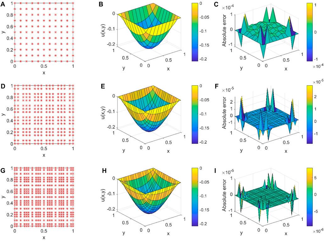
FIGURE 5. Spectral element numerical modeling for the Helmholtz equation with the interpolating polynomial order. (A) Two GLL points; (B) numerical solution with a second-order polynomial; (C) absolute error for a second-order polynomial; (D) three GLL points; (E) numerical solution with a third-order polynomial; (F) absolute error for a third-order polynomial; (G) four GLL points; (H) numerical solution with a fourth-order polynomial; and (I) absolute error for a fourth-order polynomial.

5 Model studies and discussion

5.1 Homogeneous half-space

We developed a half-space resistivity model to test the high-accuracy benchmark of our spectral element scheme. The half-space resistivity is designed as 10 $\mathrm{\Omega }\cdot \mathrm{m}$ and the computational domain is set as 20 km × 4 km. During numerical simulation, each spectral element includes 4 GLL points in the y-direction and z-direction, as shown in Figure 6. In addition, we assume that only one measuring point is located on the ground, marked by a green triangle. The numerical magnetic field H_x is simulated at f = 10 Hz.

FIGURE 6

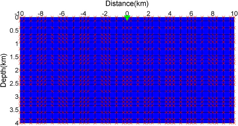
FIGURE 6. Homogeneous half-space model meshed with four GCL points per element.

We set the number of elements in the horizontal direction to 10 (i.e., N_y = 10), while the number of elements in the depth direction is designed to 5 and 10, respectively (i.e., N_z = 10 and 5). Figure 7 shows the numerical solution of the magnetic field H_x for the homogeneous half-space frequency of f = 10 Hz. They also offer that the real part and imaginary part of the magnetic field H_x calculated by the spectral element method agree with the analytical solution. This phenomenon also shows the correlation between the number of discrete elements and computational accuracy. Furthermore, it indicates that the number of discrete components does not affect the computational accuracy under high-polynomial order conditions. These results suggest that the spectral element approach can improve the accuracy for the two-dimensional magnetotelluric forward modeling.

FIGURE 7

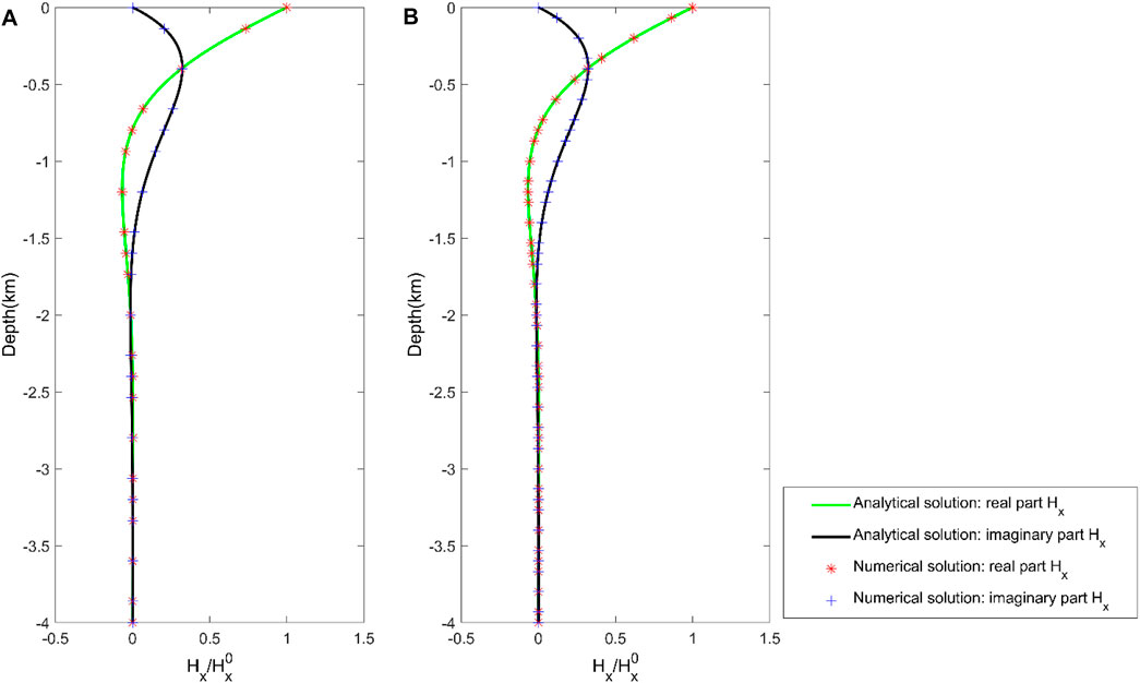
FIGURE 7. Spectral element numerical solution of magnetic field H_x for the frequency f=10 Hz in the half-space resistivity model. The number of elements in the depth direction for (A) Nz = 5 and (B) Nz = 10.

To further verify the applicability of our spectral element approach, we increase the number of elements in horizontal and depth directions to 20. We then calculated the magnetotelluric response, including apparent resistivity and phase, at f = 0.1, 1.1, 10, 10, and 100 Hz frequencies in the TM mode and TE mode. The computing time of our code is about 1.6 s for each frequency. The apparent resistivity for each frequency is identical to the true resistivity 10 $\mathrm{\Omega }\cdot \mathrm{m}$, and the phase was equal to 45°. The RMS errors of the magnetotelluric responses are given in Table 1. It is clear that the RMS error is proportional to the frequency, with the minimum error at f = 0.01 Hz and the maximum error at f = 100 Hz. In general, the RMS error value falls within the frequency band that we set, which is also the acceptable error range. The results show that our spectral element approach has high computational accuracy.

TABLE 1

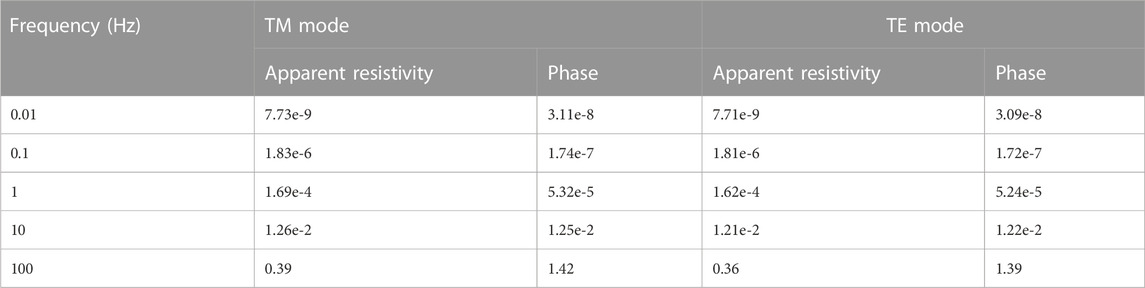
TABLE 1. RMS errors of the magnetotelluric responses for the half-space resistivity model.

5.2 COMMEMI 2D-1 model

We conducted a numerical experiment to compare with the finite difference method. This numerical experiment coincides with the COMMEMI 2D-1 example (Zhdanov et al., 1997), which can test the accuracy and reliability of the spectral element forward algorithm. The COMMEMI 2D-1 model is shown in Figure 8. A symmetrical, rectangular, low-resistivity body is inserted in a homogeneous conductive half-space. The rectangular anomaly body has a width of 1,000 m, a length of 2,000 m, and a burial depth of 250 m from the ground surface. The resistivity of the anomaly is set as $=0.5$ $\mathrm{\Omega }\cdot \mathrm{m}$, and the half-space resistivity is designed as $\rho =100$ $\mathrm{\Omega }\cdot \mathrm{m}$. The frequency we applied in the next two experiments was f = 0.1 Hz.

FIGURE 8

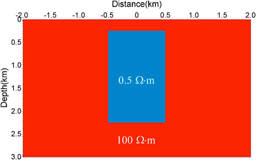
FIGURE 8. Resistivity distribution of the COMMEMI 2D-1 model.

First, we simulated the numerical solutions for the COMMEMI 2D-1 model using the spectral element algorithm and the finite difference method (Tong et al., 2018). In this example, the uniform meshes of the model for the whole calculation area are set to $\Delta y\times \Delta z=100\mathrm{m}\times 50\mathrm{m}$. For spectral element numerical modeling, each spectral element includes two GLL points in the y-direction and z-direction, and has nine points for each element. The numerical apparent resistivities and phases in the TM mode are shown in Figure 9. The results show that the numerical results calculated by the spectral element method match well with those of the finite difference method. Compared to finite difference results, the spectral element method shows a clear and continuous downward smoothness in TM mode calculations. The numerical results for the TE mode are shown in Figure 10. These results also matched well for the numerical magnetotelluric responses in the TE mode. The computing time of the COMMEMI 2D-1 model is about 0.5 s for the finite difference algorithm and about 1.8 s for the spectral element algorithm.

FIGURE 9

FIGURE 9. Comparison of numerical results for the COMMEMI 2D-1 model in the TM mode. (A) Apparent resistivities and (B) phases.

FIGURE 10

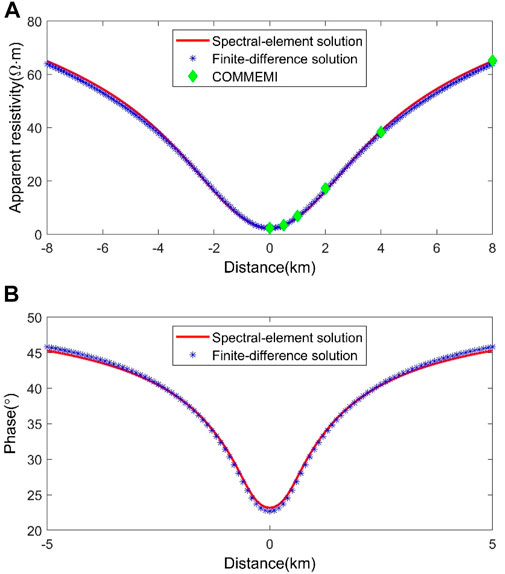
FIGURE 10. Comparison of numerical results for the COMMEMI 2D-1 model in the TE mode. (A) Apparent resistivities and (B) phases.

We also compare the numerical apparent resistivities calculated by the spectral element scheme and the finite difference approach with the averaged numerical solutions of the COMMEMI project (Zhdanov et al., 1997), showing that the numerical apparent resistivities of the spectral element scheme agree well with the averaged numerical solutions of the COMMEMI project compared to those measured by the finite difference approach (Figure 9 top; Figure 10 top). It means that the modeling precision of the spectral element scheme is higher than that of the finite difference method in calculating the magnetotelluric responses using the same mesh size.

In the second example, we only simulate the spectral element solutions with different polynomial orders in the COMMEMI locations. In this experiment, we designed a non-uniform grid of the model over the entire computational domain. To make a more precise comparison with the resistivity values published by the committee experiments, in Table 2, we list the standard deviation from Table B.11 (Zhdanov et al., 1997) along with the numerical resistivity values simulated by the spectral element approach. From Table 2, the values produced by the spectral element method match well with the numerical results published in the COMMEMI experiments. The accuracy of the apparent resistivity simulated by the spectral element might depend on the polynomial order.

TABLE 2

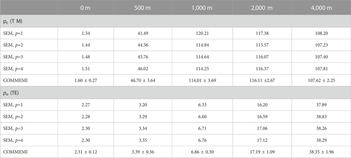
TABLE 2. Apparent resistivities simulated by the spectral element code compared to the COMMEMI results.

5.3 Topographical model

To compute the magnetotelluric responses of the two-dimensional undulating terrain, we applied our spectral element code to a ridge topographical model, as shown in Figure 11, which is the same as that used by other researchers (Wannamaker et al., 1986; Liang et al., 2021). The ridge model has a width of 2,400 m with a height of 100 m, and its resistivity value of half-space is $=100$ $\mathrm{\Omega }\cdot \mathrm{m}$. The calculated magnetotelluric responses obtained by the finite element subroutine (Wannamaker et al., 1986) are the reference for this simulation.

FIGURE 11

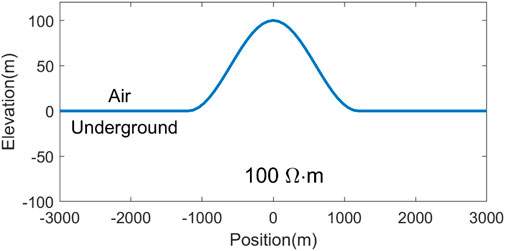
FIGURE 11. Ridge topographical model with background resistivity 100 $\mathrm{\Omega }\cdot \mathrm{m}$.

In this study, the non-uniform meshes in the TM mode and TE mode are set as 15 × 10 and 20 × 10, respectively (in which 10 km is the air media and its resistivity is equal to 10¹⁵ $\mathrm{\Omega }\cdot \mathrm{m}$), and each spectral element has four GLL points in the y-direction and z-direction. The measurement profile along the atmospheric grounding interface varies from −2,000 to 2,000 m. The frequency to be tested is only 10 Hz. Figure 12 shows the comparison of the finite element results from Wannamaker et al. (1986) and our spectral element forward code, and the results match well. The maximum relative apparent resistivity error between the two forward schemes is equal to 0.15% in the TM mode and 0.07% in the TE mode, respectively. The maximum relative phase error is equal to 0.04% in the TM mode and 0.05% in the TE mode, respectively. As shown in Figure 12A, the topographic resistivity distortion of the TE mode is smaller than that of the TM mode.

FIGURE 12

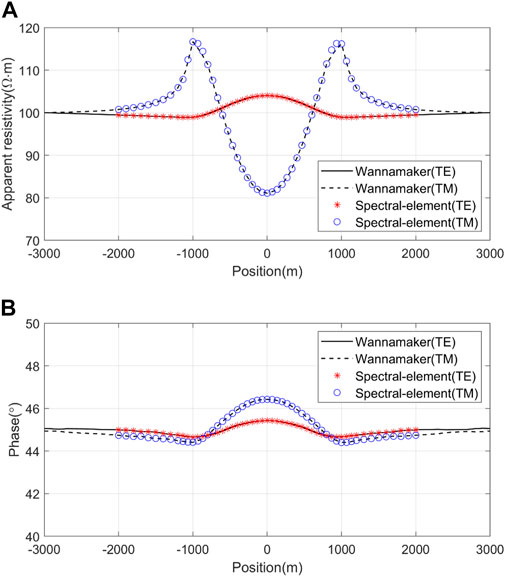
FIGURE 12. Comparison of numerical solutions for the ridge topographical model. (A) Apparent resistivities in the TM mode and TE mode; (B) phases in the TM mode and TE mode.

5.4 Smooth resistivity model

In this numerical example, a smooth resistivity model is set to 18 km × 4 km, as shown in Figure 13. We calculate the response of a two-dimensional magnetotelluric model with a smooth resistivity distribution. The least-square iterative algorithm calculated the inversion of the resistivity distribution for this model with the MT2DInvMatlab subroutine (Lee et al., 2009) for a fault model tested by Sasaki (1989).

FIGURE 13

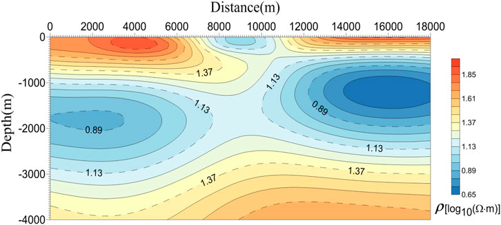
FIGURE 13. Smooth resistivity distribution inverted by the MT2DInvMatlab subroutine (Lee et al., 2009).

We chose nine frequencies to test this model, which are 0.1, 0.2, 0.5, 1.0, 2.0, 5.0, 10.0, 20.0, and 50.0 Hz (Lee et al., 2009). The computational domain was set as 200 km × 100 km, and the resistivity value for the extended region was designed as 50 $\mathrm{\Omega }\cdot \mathrm{m}$. We chose four GLL points for each element in the y-direction and z-direction, and 25 points per element. Figures 14, 15 show the pseudo-sections of the apparent resistivity and phase for this smooth model in the TM mode and the TE mode. By comparing the spectral element results and the finite element results, we found that the accuracy of the two ways is almost the same, and the results agree well.

FIGURE 14

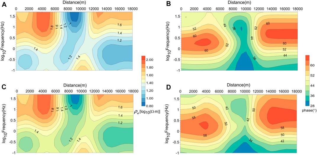
FIGURE 14. Comparison of numerical results for the smooth model. (A) TM apparent resistivity pseudo-section and (B) TM phase pseudo-section simulated by the spectral element method; (C) TM apparent resistivity pseudo-section and (D) TM phase pseudo-section simulated by the finite element method (Lee et al., 2009).

FIGURE 15

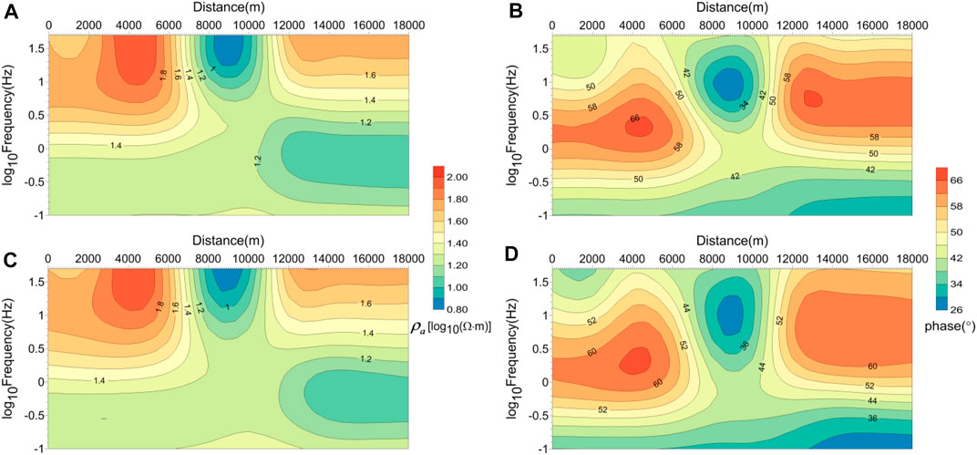
FIGURE 15. Comparison of numerical results for the smooth model. (A) TE apparent resistivity pseudo-section and (B) TE phase pseudo-section simulated by the spectral element method; (C) TE apparent resistivity pseudo-section and (D) TE phase pseudo-section simulated by the finite element method (Lee et al., 2009).

6 Conclusion

The spectral element method combined with the GLL point interpolating scheme has been developed for the first time to solve the two-dimensional magnetotelluric forward problem. We presented the spectral element formulas and implemented this algorithm. Compared with the finite difference scheme and the finite element technique, our spectral element approach requires fewer elements and produces accurate results. In the first investigation, we apply the spectral element strategy on a simple half-space geo-electric model to test its high accuracy. We presented the comparison results of the finite difference algorithm and the spectral element algorithm for the COMMEMI 2D-1 model. The accuracy of our spectral element method is better than that of the finite difference approach. We compare the numerical results from Wannamaker et al. (1986) and our spectral element scheme for a ridge topographical model, and they agree well. These results demonstrate the effectiveness and flexibility of the spectral element forward algorithm. We also applied the spectral element method to a model with a smooth resistivity structure and compared the simulation results with those of the finite element code (Lee et al., 2009). This shows that the calculation results of the spectral element algorithm are as smooth and accurate as those of the finite element method. These measurements and comparative results suggest that the spectral element method can provide another effective scheme for the two-dimensional magnetotelluric forward problem.

Data availability statement

The raw data supporting the conclusion of this article will be made available by the authors, without undue reservation.

Author contributions

All authors participated in editing and reviewing the manuscript. XT derived the linear equation system of the spectral element approach and developed the numerical simulation code. YS performed the numerical experiments and result analysis. BZ plotted some of the figures. All authors read and agreed to the submitted version of the manuscript.

Funding

This research work was partly supported by the National Natural Science Foundation of China under grants 42274083 and 41974049, and partly by the Hunan National Natural Science Foundation under Grant 2023JJ30411.

Acknowledgments

The authors would like to thank Syed Muzyan Shahzad, who modified the whole paper for English writing and gave excellent suggestions to improve the writing quality. They would also like to thank Dawei Gao for checking the numerical results of the paper. Last but not least, they thank reviewers and editors for their helpful suggestions and for improving the manuscript.

Conflict of interest

The authors declare that the research was conducted in the absence of any commercial or financial relationships that could be construed as a potential conflict of interest.

Publisher’s note

All claims expressed in this article are solely those of the authors and do not necessarily represent those of their affiliated organizations, or those of the publisher, the editors, and the reviewers. Any product that may be evaluated in this article, or claim that may be made by its manufacturer, is not guaranteed or endorsed by the publisher.

References

Avdeeva, A., Avdeev, D., and Jegen, M. (2012). Detecting a salt dome overhang with magnetotellurics: 3D inversion methodology and synthetic model studies. Geophysics 77 (4), 251–263. doi:10.1190/geo2011-0167.1

CrossRef Full Text | Google Scholar

Azeez, K. K., Patro, P. K., Harinarayana, T., and Sarma, S. V. (2017). Magnetotelluric imaging across the tectonic structures in the eastern segment of the Central Indian Tectonic Zone: Preserved imprints of polyphase tectonics and evidence for suture status of the Tan Shear. Precambrian Res. 298, 325–340. doi:10.1016/j.precamres.2017.06.018

CrossRef Full Text | Google Scholar

Barcelona, H., Favetto, A., Peri, V., Pomposiello, C., and Ungarelli, C. (2013). The potential of audio magnetotellurics in the study of geothermal fields: A case study from the northern segment of the La candelaria range, northwestern Argentina. J. Appl. Geophys. 88 (1), 83–93. doi:10.1016/j.jappgeo.2012.10.004

CrossRef Full Text | Google Scholar

Benjamin, M. L., Unsworth, J. H., Jeremy, P. R., Jean, M. L., and Legault, J. M. (2018). 3D joint inversion of magnetotelluric and airborne tipper data: A case study from the morrison porphyry Cu–Au–Mo deposit, British columbia, Canada. Geophys. Prospect. 66 (2), 397–421. doi:10.1111/1365-2478.12554

CrossRef Full Text | Google Scholar

Bihlo, A., Farquharson, C. G., Haynes, R. D., and Loredo-Osti, J. C. (2017). Probabilistic domain decomposition for the solution of the two-dimensional magnetotelluric problem. Comput. Geosci. 21 (1), 117–129. doi:10.1007/s10596-016-9598-8

CrossRef Full Text | Google Scholar

Chave, A. D., and Jones, A. G. (2012). The magnetotelluric method: Theory and practice. Cambridge: Cambridge University Press.

Google Scholar

Chen, J., Haber, E., and Oldenburg, D. W. (2002). Three-dimensional numerical modeling and inversion of magnetometric resistivity data. Geophys. J. Int. 149 (3), 679–697. doi:10.1046/j.1365-246X.2002.01688.x

CrossRef Full Text | Google Scholar

deGroot-Hedlin, C. (2006). Finite-difference modeling of magnetotelluric fields: Error estimates for uniform and nonuniform grids. Geophysics 71 (3), 97–106. doi:10.1190/1.2195991

CrossRef Full Text | Google Scholar

deGroot-Hedlin, N. C., and Constable, S. (1990). Occam's inversion generates smooth, two-dimensional models from magnetotelluric data. Geophysics 55 (12), 1613–1624. doi:10.1190/1.1442813

CrossRef Full Text | Google Scholar

Du, H. K., Ren, Z. Y., and Tang, J. T. (2016). A finite-volume approach for 2D magnetotellurics modeling with arbitrary topographies. Studia Geophys. Geod. 60 (2), 332–347. doi:10.1007/s11200-014-1041-9

CrossRef Full Text | Google Scholar

Franke, A., Börner, R. U., and Spitzer, K. (2007). Adaptive unstructured grid finite element simulation of two-dimensional magnetotelluric fields for arbitrary surface and seafloor topography. Geophys. J. Int. 171 (1), 71–86. doi:10.1111/j.1365-246X.2007.03481.x

CrossRef Full Text | Google Scholar

Gharti, H. N., Tromp, J., and Zampini, S. (2018). Spectral-infinite-element simulations of gravity anomalies. Geophys. J. Int. 215 (2), 1098–1117. doi:10.1093/gji/ggy324

CrossRef Full Text | Google Scholar

Guo, R., Li, M., Yang, F., Xu, S., and Abubakar, A. (2020). Application of supervised descent method for 2D magnetotelluric data inversion. Geophysics 85 (4), 53–65. doi:10.1190/geo2019-0409.1

CrossRef Full Text | Google Scholar

Guo, Z. Q., Egbert, G. D., and Wei, W. B. (2018). Modular implementation of magnetotelluric 2D forward modeling with general anisotropy. Comput. Geosciences 118, 27–38. doi:10.1016/j.cageo.2018.05.004

CrossRef Full Text | Google Scholar

Huang, X., Farquharson, C. G., Yin, C., Yan, L., Cao, X., and Zhang, B. (2021). A 3D forward-modeling approach for airborne electromagnetic data using a modified spectral-element method. Geophysics 86 (5), 343–354. doi:10.1190/geo2020-0004.1

CrossRef Full Text | Google Scholar

Huang, X., Yin, C., Farquharson, C. G., Cao, X., Zhang, B., Huang, W., et al. (2019). Spectral-element method with arbitrary hexahedron meshes for time-domain 3D airborne electromagnetic forward modeling. Geophysics 84 (1), 37–46. doi:10.1190/geo2018-0231.1

CrossRef Full Text | Google Scholar

Jiang, W., Duan, J., Doublier, M., Clark, A., Schofield, A., Brodie, R., et al. (2022). Application of multiscale magnetotelluric data to mineral exploration: An example from the east tennant region, northern Australia. Geophys. J. Int. 229 (2), 1628–1645. doi:10.1093/gji/ggac029

PubMed Abstract | CrossRef Full Text | Google Scholar

Kalscheuer, T., Juhojuntti, N., and Vaittinen, K. (2018). Two-dimensional magnetotelluric modelling of ore deposits: Improvements in model constraints by inclusion of borehole measurements. Surv. Geophys. 39 (3), 467–507. doi:10.1007/s10712-017-9454-y

CrossRef Full Text | Google Scholar

Kelbert, A., Meqbel, N., Egbert, G. D., and Tandon, K. (2014). ModEM: A modular system for inversion of electromagnetic geophysical data. Comput. Geosciences 66, 40–53. doi:10.1016/j.cageo.2014.01.010

CrossRef Full Text | Google Scholar

Key, K., and Weiss, C. (2006). Adaptive finite-element modeling using unstructured grids: The 2D magnetotelluric example. Geophysics 71 (6), 291–299. doi:10.1190/1.2348091

CrossRef Full Text | Google Scholar

Komatitsch, D., and Tromp, J. (1999). Introduction to the spectral element method for three-dimensional seismic wave propagation. Geophys. J. Int. 139 (3), 806–822. doi:10.1046/j.1365-246x.1999.00967.x

CrossRef Full Text | Google Scholar

Kumar, K., Gupta, P. K., and Niwas, S. (2011). Efficient two-dimensional magnetotellurics modelling using implicitly restarted Lanczos method. J. Earth Syst. Sci. 120 (4), 595–604. doi:10.1007/s12040-011-0093-2

CrossRef Full Text | Google Scholar

Lee, J. H., and Liu, Q. H. (2005). An efficient 3-D spectral-element method for Schrodinger equation in nanodevice simulation. IEEE Trans. Computer-Aided Des. Integr. Circuits Syst. 24 (2), 1848–1858. doi:10.1109/TCAD.2005.852675

CrossRef Full Text | Google Scholar

Lee, S. K., Kim, H. J., Song, Y., and Lee, C. K. (2009). MT2Dinvmatlab—A program in MATLAB and FORTRAN for two-dimensional magnetotelluric inversion. Comput. Geosciences 35 (8), 1722–1734. doi:10.1016/j.cageo.2008.10.010

CrossRef Full Text | Google Scholar

Liang, J. W., Tong, D. F., Tan, F., Jiao, Y. Y., and Yan, C. W. (2021). Two-Dimensional magnetotelluric modelling based on the numerical manifold method. Eng. Analysis Bound. Elem. 124 (1), 87–97. doi:10.1016/j.enganabound.2020.12.011

CrossRef Full Text | Google Scholar

Liao, X., Shi, Z., Zhang, Z., Yan, Q., and Liu, P. (2022). 2D inversion of magnetotelluric data using deep learning technology. Acta Geophys. 70, 1047–1060. doi:10.1007/s11600-022-00773-z

CrossRef Full Text | Google Scholar

Luo, Y., Tromp, J., Denel, B., and Calandra, H. (2013). 3D coupled acoustic-elastic migration with topography and bathymetry based on spectral-element and adjoint methods. Geophysics 78 (4), 193–202. doi:10.1190/geo2012-0462.1

CrossRef Full Text | Google Scholar

Lyu, C., Capdeville, Y., and Zhao, L. (2020). Efficiency of the spectral element method with very high polynomial degree to solve the elastic wave equation. Geophysics 85 (1), 33–43. doi:10.1190/geo2019-0087.1

CrossRef Full Text | Google Scholar

Martin, R., Chevrot, S., Komatitsch, D., Seoane, L., Spangenberg, H., Wang, Y., et al. (2017). A high-order 3D spectral-element method for the forward modelling and inversion of gravimetric data - application to the Western Pyrenees. Geophys. J. Int. 209 (1), ggx010–424. doi:10.1093/gji/ggx010

CrossRef Full Text | Google Scholar

Nagarjuna, D., Rao, C. K., Pavankumar, G., Kumar, A., and Manglik, A. (2021). Magnetotelluric evidence for an Archaean – proterozoic lithospheric assemblage within the Cambay rift basin, Western India, and its role in channeling of plume-derived fluids within the basin. Tectonophysics 818, 229064. doi:10.1016/j.tecto.2021.229064

CrossRef Full Text | Google Scholar

Pan, K., Wang, J., Hu, S., Ren, Z., Cui, T., Guo, R., et al. (2022). An efficient cascadic multigrid solver for 3-D magnetotelluric forward modelling problems using potentials. Geophys. J. Int. 230 (3), 1834–1851. doi:10.1093/gji/ggac152

CrossRef Full Text | Google Scholar

Patera, A. T. (1984). A spectral element method for fluid dynamics: Laminar flow in a channel expansion. J. Comput. Phys. 54 (3), 468–488. doi:10.1016/0021-9991(84)90128-1

CrossRef Full Text | Google Scholar

Patro, P. K. (2017). Magnetotelluric studies for hydrocarbon and geothermal resources: Examples from the asian region. Surv. Geophys. 38, 1005–1041. doi:10.1007/s10712-017-9439-x

CrossRef Full Text | Google Scholar

Pek, J., and Verner, T. (1997). Finite-difference modelling of magnetotelluric fields in two-dimensional anisotropic media. Geophys. J. Int. 128 (3), 505–521. doi:10.1111/j.1365-246X.1997.tb05314.x

CrossRef Full Text | Google Scholar

Pozrikidis, C. (2014). Introduction to finite and spectral element methods using MATLAB. New York: Chapman and Hall Press.

Google Scholar

Rao, K. P., and Babu, G. A. (2006). EMOD2D—A program in C++ for finite difference modeling of magnetotelluric TM mode responses over 2D Earth. Comput. Geosciences 32 (9), 1499–1511. doi:10.1016/j.cageo.2006.02.017

CrossRef Full Text | Google Scholar

Rodi, W., and Mackie, R. L. (2001). Nonlinear conjugate gradients algorithm for 2-D magnetotelluric inversion. Geophysics 66 (1), 174–187. doi:10.1190/1.1444893

CrossRef Full Text | Google Scholar

Sarakorn, W. (2017). 2-D magnetotelluric modeling using finite element method incorporating unstructured quadrilateral elements. J. Appl. Geophys. 139, 16–24. doi:10.1016/j.jappgeo.2017.02.005

CrossRef Full Text | Google Scholar

Sarakorn, W., and Vachiratienchai, C. (2018). Hybrid finite difference–finite element method to incorporate topography and bathymetry for two-dimensional magnetotelluric modeling. Earth, Planets Space 70 (1), 103. doi:10.1186/s40623-018-0876-7

CrossRef Full Text | Google Scholar

Sasaki, Y. (1989). Two-dimensional joint inversion of magnetotelluric and dipole-dipole resistivity data. Geophysics 54 (2), 254–262. doi:10.1190/1.1442649

CrossRef Full Text | Google Scholar

Seriani, G., and Oliveira, S. P. (2008). Dispersion analysis of spectral element methods for elastic wave propagation. Wave Motion 45 (8), 729–744. doi:10.1016/j.wavemoti.2007.11.007

CrossRef Full Text | Google Scholar

Siripunvaraporn, W., and Egbert, G. D. (2007). Data space conjugate gradient inversion for 2-D magnetotelluric data. Geophys. J. Int. 170 (3), 986–994. doi:10.1111/j.1365-246X.2007.03478.x

CrossRef Full Text | Google Scholar

Tarek, A. H., Mohamed, A. Z., Gad, E. Q., Hossam, M., Samah, E., and Yasuhiro, F. (2023). Deep heat source detection using the magnetotelluric method and geothermal assessment of the Farafra Oasis, Western Desert, Egypt. Geothermics 109, 102648. doi:10.1016/j.geothermics.2023.102648

CrossRef Full Text | Google Scholar

Tong, X., Guo, Y., and Xie, W. (2018). Finite difference algorithm on non-uniform meshes for modeling 2D magnetotelluric responses. Algorithms 11 (2), 203–217. doi:10.3390/a11120203

CrossRef Full Text | Google Scholar

Tong, X., Sun, Y., and Guo, R. (2020). A Chebyshev pseudo-spectral approach for simulating magnetotelluric TM-mode responses on 2D structures. J. Appl. Geophys. 179, 104085. doi:10.1016/j.jappgeo.2020.104085

CrossRef Full Text | Google Scholar

Trinh, R. T., Brossier, R., Metiver, L., Tavard, L., and Virieus, J. (2019). Efficient time-domain 3D elastic and viscoelastic full-waveform inversion using a spectral-element method on flexible Cartesian-based mesh. Geophysics 84 (1), 61–83. doi:10.1190/geo2018-0059.1

CrossRef Full Text | Google Scholar

Unsworth, M. (2010). Magnetotelluric studies of active continent-continent collisions. Surv. Geophys. 31 (2), 137–161. doi:10.1007/s10712-009-9086-y

CrossRef Full Text | Google Scholar

van der Vorst, H. A. (1992). Bi-CGSTAB: A fast and smoothly converging variant of Bi-cg for the solution of nonsymmetric linear systems. SIAM J. Sci. Comput. 13 (2), 631–644. doi:10.1137/0913035

CrossRef Full Text | Google Scholar

Wang, N., Tang, J., Ren, Z., Xiao, X., and Huang, X. (2019). Two-dimensional magnetotelluric anisotropic forward modeling using finite-volume method. Chin. J. Geophys. 62 (10), 3912–3922. doi:10.6038/cjg2019M0498

CrossRef Full Text | Google Scholar

Wannamaker, P. E., Stodt, J. A., and Rijo, L. (1987). A stable finite element solution for two-dimensional magnetotelluric modelling. Geophys. J. Int. 88 (1), 277–296. doi:10.1111/j.1365-246X.1987.tb01380.x

CrossRef Full Text | Google Scholar

Wannamaker, P. E., Stodt, J. A., and Rijo, L. (1986). Two-dimensional topographic responses in magnetotellurics modeled using finite elements. Geophysics 51 (11), 2131–2144. doi:10.1190/1.1442065

CrossRef Full Text | Google Scholar

Weiss, M., Kalscheuer, T., and Ren, Z. (2023). Spectral element method for 3-D controlled-source electromagnetic forward modelling using unstructured hexahedral meshes. Geophys. J. Int. 232 (2), 1427–1454. doi:10.1093/gji/ggac358

CrossRef Full Text | Google Scholar

Wittke, J., and Tezkan, B. (2014). Meshfree magnetotelluric modelling. Geophys. J. Int. 198 (2), 1255–1268. doi:10.1093/gji/ggu207

CrossRef Full Text | Google Scholar

Wittke, J., and Tezkan, B. (2021). Two-dimensional meshless modelling and TE-mode inversion of magnetotelluric data. Geophys. J. Int. 226 (2), 1250–1261. doi:10.1093/gji/ggab147

CrossRef Full Text | Google Scholar

Xu, J., Tang, J., and Xiao, X. (2022). A hybrid spectral element-infinite element approach for 3D controlled-source electromagnetic modeling. J. Appl. Geophys. 200, 104619. doi:10.1016/j.jappgeo.2022.104619

CrossRef Full Text | Google Scholar

Xu, S., and Zhou, H. (1997). Modelling the 2D terrain effect on MT by the boundary-element method. Geophys. Prospect. 45 (6), 931–943. doi:10.1046/j.1365-2478.1997.610301.x

CrossRef Full Text | Google Scholar

Yao, H., Ren, Z., Chen, H., Tang, J., Li, Y., and Liu, X. (2021). Two-dimensional magnetotelluric finite element modeling by a hybrid Helmholtz-curl formulae system. J. Comput. Phys. 443, 110533. doi:10.1016/j.jcp.2021.110533

CrossRef Full Text | Google Scholar

Yin, C., Liu, L., Liu, Y., Zhang, B., Qiu, C., and Huang, X. (2019). 3D frequency-domain airborne EM forward modelling using spectral element method with Gauss-Lobatto-Chebyshev polynomials. Explor. Geophys. 50 (5), 461–471. doi:10.1080/08123985.2019.1614162

CrossRef Full Text | Google Scholar

Zhang, K., Wei, W., Lu, Q., Dong, H., and Li, Y. (2014). Theoretical assessment of 3-D magnetotelluric method for oil and gas exploration: Synthetic examples. J. Appl. Geophys. 106, 23–36. doi:10.1016/j.jappgeo.2014.04.003

CrossRef Full Text | Google Scholar

Zhdanov, M. S., Varentsov, I. M., Weaver, J. T., Golubev, N. G., and Krylov, V. A. (1997). Methods for modelling electromagnetic fields results from COMMEMI—The international project on the comparison of modelling methods for electromagnetic induction. J. Appl. Geophys. 37 (3-4), 133–271. doi:10.1016/S0926-9851(97)00013-X

CrossRef Full Text | Google Scholar

Zhou, Y., Shi, L., Liu, N., Zhu, C., Liu, H., and Liu, Q. (2016). Spectral element method and domain decomposition for low-frequency subsurface EM simulation. IEEE Geoscience Remote Sens. Lett. 13 (4), 550–554. doi:10.1109/LGRS.2016.2524558

CrossRef Full Text | Google Scholar

Zhu, J., Yin, C., Liu, Y., Liu, Y., Liu, L., Yang, Z., et al. (2020). 3-D dc resistivity modelling based on spectral element method with unstructured tetrahedral grids. Geophys. J. Int. 220 (3), 1748–1761. doi:10.1093/gji/ggz534

CrossRef Full Text | Google Scholar

Zou, P., and Cheng, J. (2018). Pseudo-spectral method using rotated staggered grid for elastic wave propagation in 3D arbitrary anisotropic media. Geophys. Prospect. 66 (1), 47–61. doi:10.1111/1365-2478.12543

CrossRef Full Text | Google Scholar