Impact of variable seawater conductivity on ocean wave-induced electromagnetic fields simulated with finite difference method

Introduction

Oceanic waves can carry charged ions dissolved in seawater, and electromagnetic fields can be induced by the dynamo interaction of ocean waves with the geomagnetic field. The ocean wave-induced electromagnetic fields can be observed at various locations, including the seafloor, sea surface, and, sometimes, even at satellite altitudes (Crews and Futterman, 1962; Cox et al., 1978; Minami, 2017). These electromagnetic fields can provide sufficient information for the inversion of the ocean wave spectrum, which is widely used in ocean engineering and seakeeping considerations in ship design (Cieutat et al., 2003; Techet, 2005; Nielsen and Dietz, 2020). However, they will seriously interfere with natural magnetotelluric (MT) signals and reduce the quality of MT data.

In the past decades, the study of ocean wave-induced electromagnetic fields focused on the plane surface gravity waves with a fixed amplitude and frequency, which are usually considered the approximation of ocean waves. Weaver (1965) and Fraser (1966) calculated and observed the magnetic fields induced by surface gravity waves in the infinite ocean. Larsen (1971) developed a general theory of ocean wave-induced electromagnetic fields, especially long and intermediate surface gravity waves. Miles et al. (1977) established an analog model of magnetic fields induced by surface gravity waves in the laboratory. Ochadlick (1989) measured the magnetic fields generated by surface gravity waves at an aircraft. Lilley and Weitemeyer (2004a) calculated the apparent aeromagnetic wavelengths of the magnetic signals of the ocean swell. Lilley et al. (2004b) also observed the magnetic fields generated by ocean waves near the sea surface. Semkin and Smagin (2012) investigated the effect of self-induction exhibited by the ocean wave-induced electromagnetic fields. Shimizu and Utada (2015) demonstrated that the ocean wave-induced electromagnetic fields were rarely affected by the conductive subseafloor media.

It is well-known that actual ocean waves are not regular waves with a fixed amplitude and frequency but rather the sum of multiple-frequency amplitudes that exhibit a particular sea state with a significant wave height and peak period (Rasool et al., 2021). Recently, a more realistic and accurate ocean wave-induced electromagnetic field model has been proposed by combining surface gravity waves with the wave spectrum, which provides the distribution of ocean wave energy empirically (Chave, 1983; Ailliot et al., 2013; Ryabkova et al., 2019), and thus, connections between ocean wave-induced electromagnetic fields and the ocean wave spectrum are established. The electromagnetic fields generated by wind waves can be solved efficiently using wind speed and significant wave height, and other parameters (Yaakobi et al., 2011). Meanwhile, many studies focus on the wind-driven electromagnetic fields at different wind speeds (Zhu and Xia, 2014; Zhan and Pan, 2019). To the best of our knowledge, the electromagnetic fields generated by both the swell and mixed ocean waves have not been discussed in the literature.

In the aforementioned studies, seawater conductivity is often assumed to be constant. However, seawater conductivity is variable in the realistic ocean (Zheng et al., 2018). Previous studies have shown that there is an approximately linear relationship between seawater conductivity and temperature, and the salinity of seawater also influences the conductivity of seawater. Both the salinity and temperature of ocean water can exhibit significant spatial and temporal variations, thereby leading to variations in sea water conductivity. The mean conductivity of seawater is approximately 3.3–4 S/m, while it may reach 6 S/m above the main thermocline. Chave and Luther (1990) and Irrgang et al. (2016) investigated the effect of vertically varying seawater conductivity on ocean current-induced electromagnetic fields. As far as we know, the impact of changes in seawater conductivity on the ocean wave-induced electromagnetic fields has not been well-investigated.

In this paper, we simulate the ocean wave-induced electromagnetic fields with variable seawater conductivity using the finite difference method. The impact of variable seawater conductivity will be investigated, especially within the main thermocline at different seasons and latitudes. Then, the wave spectra of wind waves, swell, and mixed waves are presented and the characteristics of the electromagnetic fields are analyzed.

Methodology

FD simulation of surface gravity wave-induced electromagnetic fields

The electromagnetic fields induced by surface gravity waves can be obtained by solving the motional induction equation. Here, we adopt two-dimensional surface waves propagating in the x-direction, with no variation in the y-direction. The z-axis points downward, and the origin of the Cartesian coordinate system is at the averaged sea surface. We assume that seawater is incompressible and flow is irrotational. This means that there exists a velocity potential $\mathrm{\Phi }$ for the flow. The velocity potential $\mathrm{\Phi }$ is a harmonic function that obeys the following Laplace equation:

${\nabla }^2\mathrm{\Phi }=0,(1)$

where $\mathrm{\Phi }$ can be expressed as follows (Larsen, 1971):

$\mathrm{\Phi }=\frac{ag}{\omega }\frac{\cosh \left[p\left(d-z\right)\right]}{\cosh \left(pd\right)}{e}^{i\left(\omega t-px\right)},(2)$

where $a$ is the height of the ocean wave, the acceleration of gravity $g$ equals to 9.8 $m/s^2$, and $p$ and $\omega$ indicate the wave number and angular frequency of the ocean wave, respectively. The dispersion relation of the ocean wave can be expressed as (Larsen, 1971)

${\omega }^2=gp\tanh \left(pd\right).(3)$

The gradient of the velocity potential $\mathrm{\Phi }$ is the flow velocity $\overrightarrow{V}$, i.e., we have

$\overrightarrow{V}=\nabla \mathrm{\Phi }.(4)$

From Eqs. 2 and 4, we get the velocity field of the ocean wave:

$\overrightarrow{V}=-\mathrm{R}\mathrm{e}\left[\frac{agpi}{\omega }\frac{\cosh \left[p\left(d-z\right)\right]}{\cosh \left(pd\right)}{e}^{i\left(\omega t-px\right)}\right]\overrightarrow{i}-\mathrm{R}\mathrm{e}\left[\frac{agp}{\omega }\frac{\sinh \left[p\left(d-z\right)\right]}{\cosh \left(pd\right)}{e}^{i\left(\omega t-px\right)}\right]\overrightarrow{k},(5)$

where $\overrightarrow{i}$ and $\overrightarrow{k}$ are the unit vectors in the x- and z-directions, respectively. $\mathrm{R}\mathrm{e}$ indicates the real part of a complex function.

The frequency domain Maxwell equations in the quasi-stationary state approximation can be written as

$\left\{\begin{array}{l}\nabla \times \overrightarrow{H}-\sigma \overrightarrow{E}=\sigma \left(\overrightarrow{V}\times \overrightarrow{F}\right),\\ \nabla \times \overrightarrow{E}+i\omega \mu \overrightarrow{H}=0,\\ \nabla \cdot \overrightarrow{H}=0,\end{array}\right.(6)$

where $\overrightarrow{E}$ is the in situ electric field, $\overrightarrow{H}$ is the magnetic field, $\sigma$ is the conductivity, and $\mu$ is the magnetic permeability, which is assumed to be equal to the permeability of free space. $\overrightarrow{F}$ is the ambient geomagnetic field given by

$\overrightarrow{F}=F_0\left(\cos I\cos \theta \overrightarrow{i}-\cos I\sin \theta \overrightarrow{j}+\sin I\overrightarrow{k}\right),(7)$

where $\overrightarrow{i},\overrightarrow{j},\mathrm{a}\mathrm{n}\mathrm{d}\overrightarrow{k}$ are the unit vectors in the positive directions of x-, y- and z-axes, respectively. $F_0$ is the intensity of the geomagnetic field, and $\theta$ and $I$ are the declination and inclination of the geomagnetic field, respectively.

Taking the curl of first equation of Eq. 6 and eliminating $\overrightarrow{E}$ with the use of the second equation of Eq. 6, yields

$\nabla \times \nabla \times \overrightarrow{H}+i\omega \mu \sigma \overrightarrow{H}=\sigma \nabla \times \left(\overrightarrow{V}\times \overrightarrow{F}\right)+\nabla \sigma \times \left(\overrightarrow{V}\times \overrightarrow{F}+\overrightarrow{E}\right).(8)$

Compared to the spatial variability of ocean waves $\overrightarrow{V}$, the variations in the geomagnetic field $\overrightarrow{F}$ are small and can be ignored. By using $\nabla \cdot \overrightarrow{F}=0$ and $\nabla \cdot \overrightarrow{V}=0$, Eq. 8 can be rewritten as

${\nabla }^2\overrightarrow{H}-i\omega \mu \sigma \overrightarrow{H}=-\sigma \left[\left(\overrightarrow{F}\cdot \nabla \right)\overrightarrow{V}\right]-\nabla \sigma \times \left(\overrightarrow{V}\times \overrightarrow{F}+\overrightarrow{E}\right).(9)$

Since the impact of the conductivity of the subseafloor material on the electromagnetic fields within the frequency range of ocean waves at and above the seabed is negligible (Larsen, 1971; Minami and Toh, 2013; Shimizu and Utada, 2015), an air–seawater–seafloor three-layer conductivity model, as shown in Figure 1, is considered here. Assuming that the conductivity of air is ${\sigma }_0$, the conductivity and thickness of seawater are ${\sigma }_1$ and $d$, respectively, and the conductivity of the seafloor medium is ${\sigma }_2$.

FIGURE 1

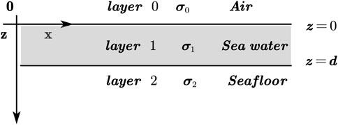
FIGURE 1. Horizontally three-layered conductivity model.

Since the forcing term of $\overrightarrow{V}$ is harmonic in time $t$ and $x$, the electromagnetic fields resulting from $\overrightarrow{V}$ have a similar harmonic form as $\overrightarrow{H}\propto \exp \left(i\omega t-ipx\right)$ and $\overrightarrow{E}\propto \exp \left(i\omega t-ipx\right)$ (Weaver, 1965; Håland et al., 2012). Hence, Eq. 9 can be rewritten as

$\frac{{\partial }^2\overrightarrow{H}}{\partial z^2}-m_j^2\overrightarrow{H}=-\sigma \left[\left(\overrightarrow{F}\cdot \nabla \right)\overrightarrow{V}\right]-\nabla \sigma \times \left(\overrightarrow{V}\times \overrightarrow{F}+\overrightarrow{E}\right),(10)$

where $m_j=\sqrt{p^2+i\omega \mu {\sigma }_j}$ is the wave number in the $j^{th}$ layer $\left(j=\mathrm{0,1,2}\right)$. The first term on the right-hand side of Eq. 10 represents the influence of the source term, and the second term indicates the influence of the change in seawater conductivity.

For the length scale of ocean waves, the horizontal variation in seawater conductivity is negligible compared to its vertical variations (Chave and Luther, 1990; Tyler et al., 2017). Hence, Eq. 10 can be simplified as (Minami et al., 2021)

$\left(\frac{{\partial }^2}{\partial z^2}-m_j^2\right)\left(\begin{array}{c}{H}_x\\ H_z\end{array}\right)=\left(\begin{array}{c}-{\sigma }_j\left(F_x\frac{\partial }{\partial x}+F_z\frac{\partial }{\partial z}\right)V_x-\frac{\partial {\sigma }_j}{\partial z}\left(V_z{F}_x-V_x{F}_z+E_y\right)\\ -{\sigma }_j\left(F_x\frac{\partial }{\partial x}+F_z\frac{\partial }{\partial z}\right)V_z\end{array}\right).(11)$

The magnetic fields in the air can be expressed as

$\left(\begin{array}{c}{H}_x\\ H_z\end{array}\right)=\left(\begin{array}{c}{P}_a\exp \left(m_{0}z\right)\\ R_a\exp \left(m_{0}z\right)\end{array}\right),(12)$

where $P_a$ and $R_a$ are the coefficients to be determined.

Similarly, the magnetic fields in the seafloor layer can be expressed as

$\left(\begin{array}{c}{H}_x\\ H_z\end{array}\right)=\left(\begin{array}{c}{P}_s\exp \left(-m_{2}z\right)\\ R_s\exp \left(-m_{2}z\right)\end{array}\right),(13)$

where $P_s$ and $R_s$ are the coefficients in the seafloor layer to be determined.

At the air–ocean interfaces $\left(z=0\right)$ and the seafloor $\left(z=d\right)$, both the tangential $\left(H_x\right)$ and normal $\left(H_z\right)$ components of the magnetic field are continuous. The induced magnetic field tends to be zero as z approaches $\pm \infty$. Using the third equation of Eqs 6, 12, 13, we have the boundary conditions on both the sea surface and seafloor:

$\left\{\begin{array}{c}\frac{\frac{d{H}_z\left(0\right)}{dz}}{H_z\left(0\right)}=m_0,\\ \frac{\frac{d{H}_z\left(d\right)}{dz}}{H_z\left(d\right)}=-m_2.\end{array}\right.(14)$

The boundary value problems (11) and (14) can be solved using the finite difference method. We consider that the one-dimensional grid and the space from the sea surface to the seafloor are spatially discretized into $N$ equally spaced elements. The step size is $h=\frac{d}{N}$, and each spatial point is defined by $z_i=ih,i=\mathrm{0,1},\cdots \cdots N$.

Using the Taylor series expansion, the second derivative of the normal $\left(H_z\right)$ component of the magnetic field can be approximated by

$f^{″}\left(z_i\right)\approx \frac{f\left(z_{i+1}\right)-2f\left(z_i\right)+f\left(z_{i-1}\right)}{h^2}-\frac{h^2}{12}{f}^{\left(4\right)}\left({\xi }_i\right),z_{i-1}<{\xi }_i<z_i,i=\mathrm{1,2}\cdots ,N-1.(15)$

Eq. 11 can then be approximated using the symmetric difference equation

$\frac{1}{h^2}\left(f_{i-1}-2f_i+f_{i+1}\right)+q_i{f}_i\approx g_i,i=\mathrm{1,2}\cdots ,N-1,(16)$

with

$q_i=-\left(p^2+i\omega \mu {\sigma }_{1,i}\right),g_i=-{\sigma }_{1,i}\left(F_x\frac{\partial }{\partial x}+F_z\frac{\partial }{\partial z}\right)V_{z,i}.(17)$

The first derivative of the magnetic field component $f^{\prime }\left(z\right)$ at the sea surface $\left(z=z_0\right)$ and seafloor $\left(z=z_N\right)$ can be approximated by

$\left\{\begin{array}{l}{f}^{\prime }\left(z_0\right)\approx \frac{-3f\left(z_0\right)+4f\left(z_1\right)-f\left(z_2\right)}{2h}+\frac{h^2}{3}{f}^{‴}\left({\xi }_0\right),z_0<{\xi }_0<z_2,\\ f^{\prime }\left(z_N\right)\approx \frac{f\left(z_{N-2}\right)-4f\left(z_{N-1}\right)+3f\left(z_N\right)}{2h}+\frac{h^2}{3}{f}^{‴\left({\xi }_N\right)},z_{N-2}<{\xi }_N<z_N.\end{array}\right.(18)$

The boundary conditions in Eq. 14 become

$\left\{\begin{array}{l}-m_0{f}_0+\frac{-3f_0+4f_1-f_2}{2h}=0,\\ m_2{f}_N+\frac{f_{N-2}-4f_{N-1}+3f_N}{2h}=0.\end{array}\right.(19)$

One obtains a linear system of N-1 equations, which can be written in the following matrix form:

$\left[\begin{array}{ccccc}{q}_1-\frac{2}{h^2}+\frac{4}{\left(2h{m}_0+3\right)h^2}& \frac{1}{h^2}-\frac{1}{\left(2h{m}_0+3\right)h^2}& 0& \cdots & 0\\ \frac{1}{h^2}& q_2-\frac{2}{h^2}& \frac{1}{h^2}& \cdots & 0\\ \cdots & \cdots & \cdots & \cdots & \cdots \\ 0& \cdots & \frac{1}{h^2}& q_{N-2}-\frac{2}{h^2}& \frac{1}{h^2}\\ 0& \cdots & \frac{1}{2h}& \frac{1}{h^2}-\frac{1}{h^2\left(3+2h{m}_2\right)}& q_{N-1}-\frac{2}{h^2}+\frac{4}{\left(3+2h{m}_2\right)h^2}\end{array}\right]\times \left[\begin{array}{c}{f}_1\\ f_2\\ ⋮\\ f_{N-2}\\ f_{N-1}\end{array}\right]=\left[\begin{array}{c}{g}_1\\ g_2\\ ⋮\\ g_{N-2}\\ g_{N-1}\end{array}\right].(20)$

The aforementioned equations can be solved by using a direct solver to obtain $H_z$, and $H_x$ and $E_y$ can be computed from $H_z$:

$\left\{\begin{array}{l}{H}_x=\frac{1}{ip}\frac{\partial }{\partial z}{H}_z,\\ E_y=\frac{\omega \mu }{p}{H}_z.\end{array}\right.(21)$

It should be noted that the electric fields calculated in this section are in situ electric fields. The geomagnetic electro-kinetograph field $\overrightarrow{E^{\prime }}$, observed by the observer moving with the fluid velocity, can be referred to (Larsen, 1971)

$\overrightarrow{E^{\prime }}=\overrightarrow{E}+\overrightarrow{V}\times \overrightarrow{F}.(22)$

The magnetic induction intensity $\overrightarrow{B}$ can be described as

$\overrightarrow{B}=\mu \overrightarrow{H}.(23)$

Validation of FD simulation

In order to validate the accuracy of the finite difference (FD) algorithm described in the previous section, we simulated the wave-induced electromagnetic fields in the model, as shown in Figure 1. The conductivity in the air is set to be $10^{-8}S/m$. The conductivity and depth of seawater are 3.33 S/m and 200 m, respectively, and the seafloor conductivity is supposed to be 1 S/m. The amplitude and frequency of the surface gravity wave are set to be 1 m and 0.1 Hz, respectively. The ambient geomagnetic field is $F_0=45000nT$, and the declination $\theta =30°$ and inclination $I=60°$. The finite difference grid is a uniform grid with a grid spacing of 0.05 m.

Figure 2 shows the amplitudes of ocean wave-induced electrical and magnetic field components obtained using the FD method. For comparison, the analytic solutions calculated using the formulae used by Shimizu and Utada (2015) are also shown. The FD numerical results agree very well with the analytic solutions. The relative errors of all three components (Ey, Bx, and Bz) are below 0.5%. Figure 2shows that 1) the amplitudes of both $B_z$ and $E_y$ components near the sea surface are much larger and decrease exponentially with increasing$\left|z\right|$. The attenuation of both $B_z$ and $E_y$ in seawater is faster than that in the air; 2) the horizontal magnetic component $B_x$ exhibits two peaks, one at the sea surface and the other in the seawater.

FIGURE 2

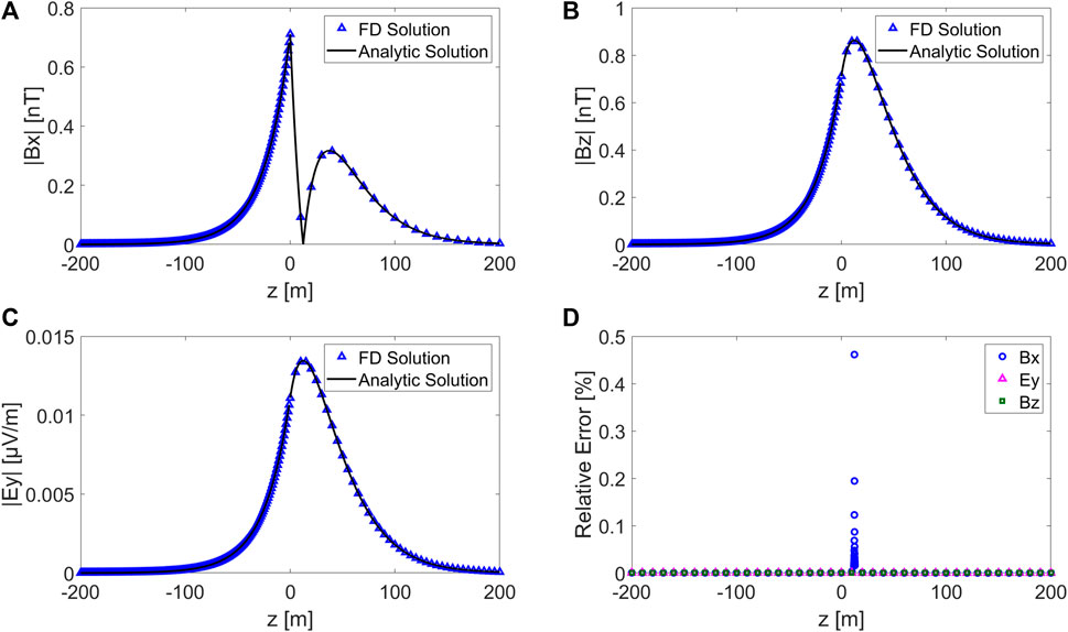
FIGURE 2. Amplitudes of electromagnetic fields induced by ocean waves; the blue triangles and the black solid line represent the FD results and analytic solution, respectively. Bx (A), Bz (B), Ey (C), and relative errors (D).

Impact of variable seawater conductivity on ocean wave-induced electromagnetic fields

Generally, the conductivity of seawater decreases with the depth of the ocean. It may exhibit either a linear or exponential decrease. In this section, we evaluate how seawater conductivity affects the electromagnetic field generated by ocean waves in both linear and exponential models. Additionally, we utilize empirical formulas to calculate the ocean wave-induced electromagnetic field while also factoring in the effects of the thermocline layer. In the following numerical simulation, the amplitude and frequency of the surface gravity wave are set to be 1 m and 0.1 Hz, respectively.

The effect of the depth-averaged seawater conductivity

To investigate the impacts of seawater conductivity distribution on ocean wave-induced electromagnetic fields, we conducted modeling studies for two cases. In the first case, the seawater conductivity is set to be a constant of 3 S/m, 4 S/m, and 5 S/m. In the second case, seawater conductivity linearly varies with depth z, with a depth-averaged conductivity of 3 S/m, 4 S/m, and 5 S/m (Figure 3A). The ambient geomagnetic field is $F_0=45000nT$, and the declination $\theta =30°$ and inclination $I=60°$.

FIGURE 3

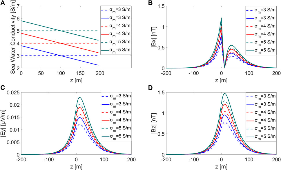
FIGURE 3. (A) Seawater conductivity profiles of six conductivity distributions; vertical profiles with different depth-averaged conductivity distributions are presented for (B) Bx, (C) Ey, and (D) Bz.

Figures 3B–D show the ocean wave-induced electromagnetic fields with different seawater conductivity distributions. One can see that 1) maintaining a constant depth-averaged seawater conductivity but changing from a uniform to a linear distribution with depth results in an increase in the induced electromagnetic fields. Here, the variations in seawater conductivity distribution led to an increase of up to 25% in the electromagnetic fields; 2) for a fixed seawater conductivity distribution (i.e., a constant gradient of linear conductivity variation), changes in the depth-averaged seawater conductivity also affect the induced electromagnetic field. It is evident that the induced electromagnetic field increases with the increase in the depth-averaged seawater conductivity.

The effect of the seawater conductivity gradients

To investigate the effects of the seawater conductivity gradients, we consider the model with the same depth-averaged conductivity but different conductivity gradients. The depth-averaged conductivity gradient ${\sigma }_g$ can be defined as

${\sigma }_g=\frac{1}{d}{\int }_0^d\left|\frac{d\sigma \left(z\right)}{dz}\right|dz.(24)$

Figure 4A shows the variation in seawater conductivity for depth-averaged conductivity gradients of 0.0025, 0.006, and 0.011. As shown in Figures 4B–D, the induced electromagnetic fields increase with the increase in the depth-averaged conductivity gradient.

FIGURE 4

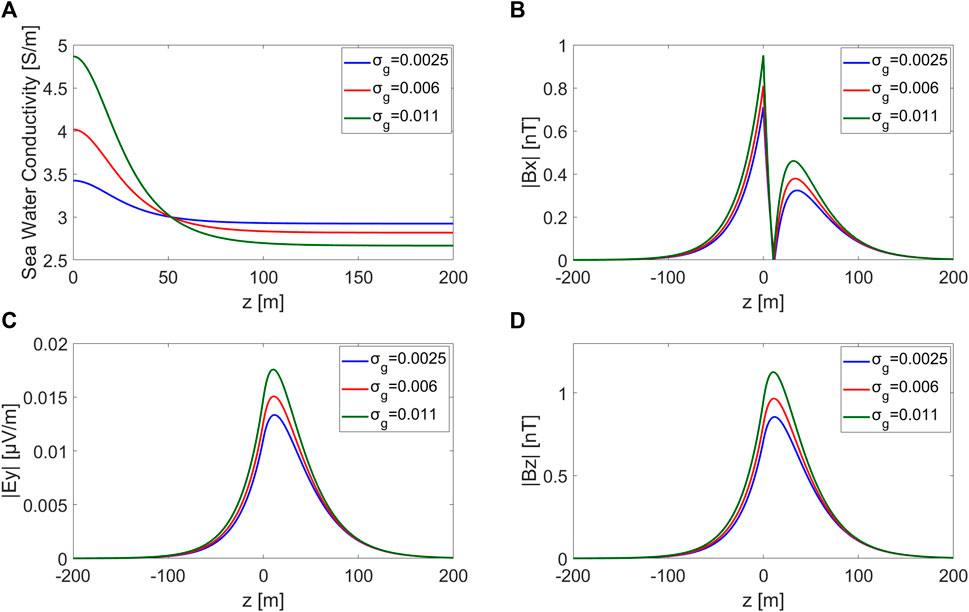
FIGURE 4. (A) Seawater conductivity with different depth-averaged conductivity gradients; (B) Bx, (C) Ey, and (D) Bz.

The effect of the thermocline

The thermocline is the transition layer between the warmer mixed water near the surface and the cooler deep water below. It plays an important role in marine ecology, meteorological forecasting, underwater communication, and aquaculture. In the body of the thermocline, there is a sudden temperature change. The temperature decreases rapidly from the mixed layer to the cooler deep layer.

The temperature t, salinity S, and pressure p in seawater affect the variations in seawater conductivity. According to the 1978 Practical Salinity Scale (Fofonoff and Millard, 1983), the seawater conductivity $C\left(S,t,p\right)$ can be expressed as

$C\left(S,t,p\right)=C\left(\mathrm{35,15,0}\right)R\left(S,t,p\right),(25)$

where $R\left(S,t,p\right)$ is the conductivity ratio, and $C\left(\mathrm{35,15,0}\right)$ represents the conductivity of standard seawater at a salinity of $35‰$, a temperature of 15°C, and standard atmospheric pressure (0 dbar), with a value of 4.2914$S/m$.

The conductivity ratio $R\left(S,t,p\right)$ can be written as

$R\left(S,t,p\right)=\frac{1}{2A}\left[\sqrt{{\left(B-A{r}_t{R}_t\right)}^2+4r_t{R}_{t}A\left(B+C\right)}-\left(B-A{r}_t{R}_t\right)\right](26)$

with

$r_t=0.6766097+0.0200564t+1.104259\times 10^{-4}{t}^2-6.9698\times 10^{-7}{t}^3+1.0031\times 10^{-9}{t}^4,(27)$

$\begin{array}{c}A=0.4215-0.003107t,\\ B=1+0.03426t+4.464\times 10^{-4}{t}^2,\\ C=\left(2.07\times 10^{-5}-6.37\times 10^{-10}p+3.989\times 10^{-15}{p}^2\right)p.\end{array}(28)$

The factor $R_t\left(S,t\right)$ can be calculated from the salinity S and the temperature t as

$\begin{array}{l}S=0.008+0.0005c-\left(0.1692+0.0056c\right)R_t^{1/2}\\ +\left(25.3851-0.0066c\right)R_t+\left(14.04941-0.0375c\right)R_t^{3/2}\\ +\left(-7.0261+0.0636c\right)R_t^2+\left(2.7081-0.0144c\right)R_t^{5/2}\end{array}(29)$

with

$c=\frac{t-15}{1+0.0162\left(t-15\right)}.(30)$

As a high linear correlation exists between temperature and conductivity in the thermocline, the conductivity in it may include the temperature dependence only and a constant salinity of 36 psu can be considered in Eq. 29 (Tyler et al., 2017; Zheng et al., 2018).

The thermocline largely depends on the seasons and latitudes. Figure 5 displays the variation in temperature and seawater conductivity in the thermocline for different latitudes (Figure 5A) and different seasons (Figure 5B). The temperature profiles vary at different latitudes as the surface water is warmer near the equator and colder at the poles. In low-latitude tropical regions, the sea surface is much warmer, leading to a highly pronounced thermocline, while in polar regions, the temperature is fairly constant at all depths. Seasons also have an impact on the vertical variation in seawater temperature and conductivity. In winter, the sea surface temperature is lower than that in summer, resulting in a thicker thermocline. In contrast, in summer, due to solar radiation, the thermocline is thinner and has more pronounced variations.

FIGURE 5

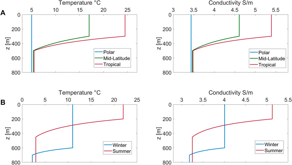
FIGURE 5. (A) Representative temperature and corresponding conductivity profiles for tropical, mid-latitude, and polar regions, and for (B) winter and summer.

The geomagnetic field also varies with latitudes. The intensity of the magnetic field is generally higher near the magnetic poles and lower near the equator. At the magnetic equator, where the proximity to the geographic equator is high, the magnetic field lines intersect Earth’s surface, resulting in a smaller magnetic inclination angle. However, as the latitude increases, the magnetic inclination angle gradually becomes larger (Table 1).

TABLE 1

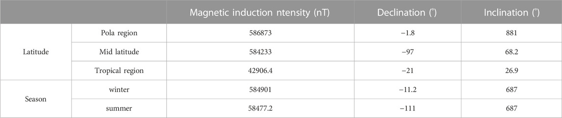
TABLE 1. Geomagnetic field intensity, magnetic declination, and inclination vary with latitudes (polar, mid-latitude, and tropical regions) and seasons (summer and winter).

Figure 6 shows the electromagnetic fields in the thermocline for tropical, mid-latitude, and polar regions, and for winter and summer, respectively. Figure 6 shows that 1) compared to tropical and polar regions, the mid-latitude regions have the highest amplitude values of induced electromagnetic fields (Figure 6A). This is because tropical regions have relatively high seawater conductivity but low geomagnetic field values, while mid-latitude regions have slightly lower seawater conductivity than tropical regions but significantly higher geomagnetic field values; 2) due to the relatively insignificant seasonal variations in the geomagnetic field, the values of induced electromagnetic fields are larger in summer than those in winter (Figure 6B).

FIGURE 6

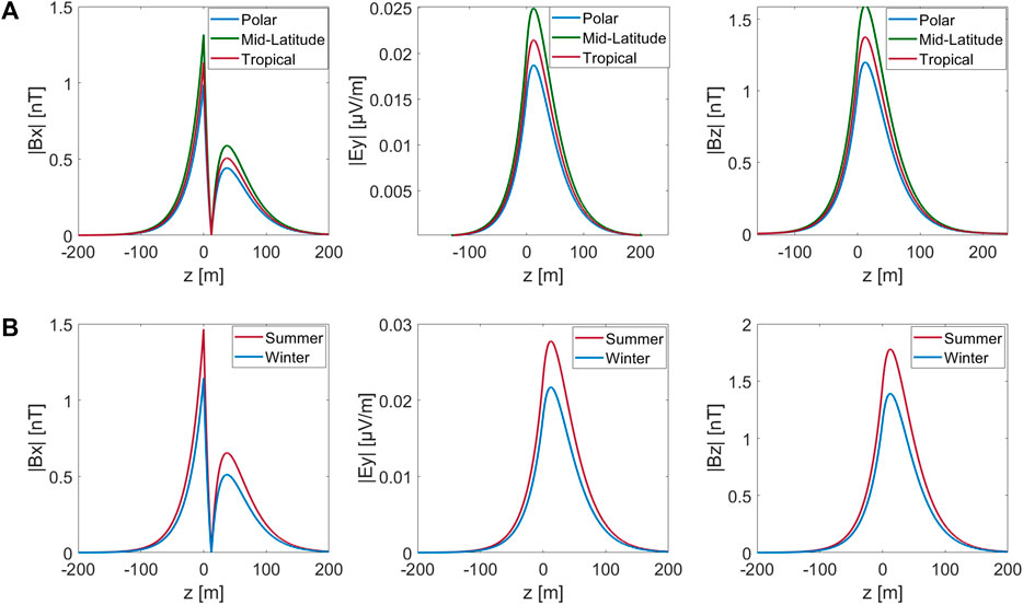
FIGURE 6. (A) Induced electromagnetic fields of ocean waves in thermoclines for tropical, mid-latitude, and polar regions and (B) for winter and summer, respectively.

Numerical simulation of electromagnetic fields induced by ocean wave based on sea wave spectrums within inhomogeneous ocean

The motion of realistic ocean waves can be described as a stationary random process. The ocean waves can be simulated by the wave spectrum, which represents the statistical characteristic of ocean wave motion (Longuet-Higgins, 1962; Grainger et al., 2021). Thus, the height and velocity potential of the ocean waves can be simulated by linear superposition:

$\eta \left(x,t\right)=\mathrm{R}\mathrm{e}{\displaystyle \sum _{k=1}^N}{a}_k\exp \left[i\left({\omega }_{k}t-p_{k}x-{ϵ}_k\right)\right],(31)$

$\mathrm{\Phi }\left(x,t\right)={\displaystyle \sum _{k=1}^N}\frac{a_{k}g}{\omega }\frac{\cosh \left[p\left(d-z\right)\right]}{\cosh \left(pd\right)}\exp \left[i\left({\omega }_{k}t-p_{k}x-{ϵ}_k\right)\right],(32)$

where $a_k$, ${\omega }_k$, and $p_k$ are the amplitude, angular frequency, and wave number for each component of the ocean wave, respectively. $N$ is the number of frequencies. The phase ${ϵ}_k$ is randomly distributed within the interval $\left[\mathrm{0,2}\pi \right]$. The amplitude $a_k$ can be expressed as (Zhu and Xia, 2014)

$a_k=\sqrt{2S\left(w_k\right)∆{\omega }_k},(33)$

where $S\left(w_k\right)$ is the spectrum of the ocean wave and $∆{\omega }_k$ is the interval of the angular frequency.

We consider the wave-induced electromagnetic field in a specific area of the South China Sea, taking into account the actual temperature, salinity, and density of seawater. The area is located at latitude 18°N and longitude 119.336°E. The water depth in this region is 294 m. The seawater conductivity can be calculated using Eqs 25–30. Figure 7 shows the distribution of temperature, salinity, and seawater conductivity in this area. The geomagnetic induction intensity in this region is 40,174.6 nT with a magnetic declination of 47° and a magnetic inclination of 1.1°.

FIGURE 7

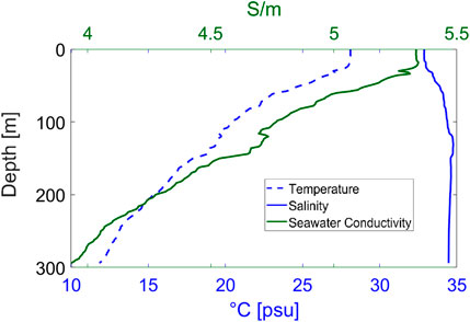
FIGURE 7. Distribution of temperature (the blue dashed line), salinity (the blue solid line), and seawater conductivity (the greed solid line) in a certain area of the South China Sea.

Electromagnetic fields induced by wind waves

The JONSWAP spectrum is commonly used to describe the spectrum of wind waves (Hasselmann et al., 1973):

$S\left(\omega \right)=\frac{\alpha g^2}{{\omega }^5}\exp \left[-\frac{5}{4}{\left(\frac{{\omega }_p}{\omega }\right)}^4\right]{\gamma }^r(34)$

with

$r=\exp \left[-\frac{{\left(\omega -{\omega }_p\right)}^2}{2{\tau }^2{\omega }_p^2}\right],\alpha =0.076{\left(\frac{V_{10}^2}{gx}\right)}^{0.22},{\omega }_p=22{\left(\frac{g^2}{V_{10}x}\right)}^{1/3},\tau =\left\{\begin{array}{c}0.07\omega ⩽{\omega }_p,\\ 0.09\omega >{\omega }_p,\end{array}\right.(35)$

where $\alpha$ is the energy scale factor, ${\omega }_p$ is the peak wave frequency, and $\gamma$ is the peak shape parameter. $V_{10}$ is the wind speed at a height of 10 m above the sea surface, and $x$ is the distance over which the wind blows with a constant velocity, also called wind fetch.

Figure 8 shows that with the increase in both the wind speed and wind fetch, the magnitude of the spectrum increases but the peak frequency decreases.

FIGURE 8

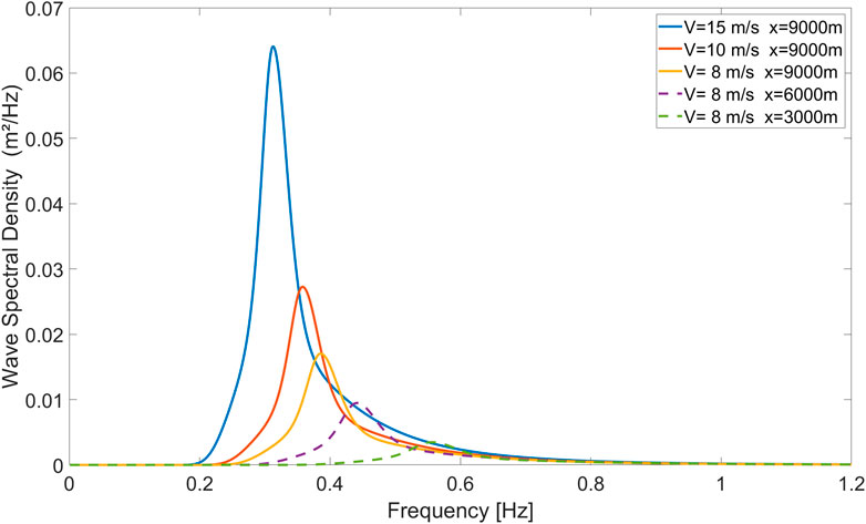
FIGURE 8. JONSWAP spectrum for different wind speeds and fetches V = 15 m/s and x = 9,000 m (the blue solid line); V = 10 m/s and x = 9,000 m (the red solid line); V = 8 m/s and x = 9,000 m (the yellow solid line); V = 8 m/s and x = 6,000 m (the purple dashed line); and V = 8 m/s and x = 3,000 m (the green dashed line).

The wind-induced electromagnetic fields at the sea surface can be obtained by combining Eqs 20, 23, 32 with the JONSWAP spectrum (34) and are depicted in Figure 9. One can observe that 1) the amplitude of the induced electric and magnetic fields increases with the increase in wind speed; 2) the magnitude of the electrical and magnetic fields increases with the expansion of the wind fetch; 3) as the wind speed increases and the wind fetch expands, the dominant peak frequency gradually shifts toward lower frequencies; and 4) the wind-induced electromagnetic fields are considerably smaller in magnitude at the seafloor (dashed lines) than those near the sea surface (solid lines).

FIGURE 9

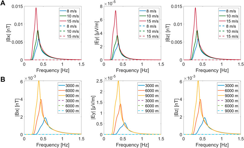
FIGURE 9. Electromagnetic fields generated with the (A) wind speed of 8 m/s, 10 m/s, and 15 m/s (a wind fetch of 9,000 m) and the (B) wind fetch of 3,000, 6,000, and 9,000 m (a wind speed of 8 m/s).

Electromagnetic fields induced by a swell

Wind waves travel in a great circle route after being generated, and after moving out of the area of the wind fetch, the waves are called swell waves and can travel thousands of kilometers. As short-wavelength waves carry less energy and dissipate faster, swell waves often have a relatively long wavelength (Gao et al., 2022). The swell spectrum is given by (Lucas and Guedes Soares, 2015)

$S\left(\omega \right)=\beta {\left(\frac{\omega }{{\omega }_p}\right)}^{-5}\exp \left[-1.25{\left(\frac{\omega }{{\omega }_p}\right)}^{-4}\right]{{\gamma }_S}^r(36)$

with

$r=\exp \left[\frac{-{\left(\omega -{\omega }_p\right)}^2}{2{\tau }^2{\omega }_p^2}\right],\tau =\left\{\begin{array}{c}0.07\omega ⩽{\omega }_p\\ 0.09\omega >{\omega }_p\end{array}\right.,\beta =\frac{5H_s^2}{16{\omega }_p}{\left[1.15+0.1688{\gamma }_S-\frac{0.925}{\left(1.909+{\gamma }_S\right)}\right]}^{-1},(37)$

where ${\omega }_p$ is the peak wave frequency, ${\gamma }_S$ is the peak shape parameter, and $H_s$ is the significant wave height. We assume ${\omega }_p=0.3142rad/s$ and $H_s=5m$. Figure 10 shows the spectrum of swell waves for three different peak shape parameters ${\gamma }_S=2$, 5, and 8.

FIGURE 10

FIGURE 10. Swell spectrum for three different peak shape parameters γ_S = 2, 5, and 8, and H_S = 5 m, and ω_P = 0.3142 rad/s.

Figure 10 shows that with the increase in the shape peak parameter ${\gamma }_S$, the amplitude of the swell spectrum increases but results in a narrower band of the spectrum.

Figure 11 shows the electromagnetic fields generated by the ocean swell at both the sea surface (A) and seafloor (B). Figure 11 shows that 1) as the shape peak parameter ${\gamma }_S$ increases, the magnitudes of the electromagnetic fields also increase at both the sea surface and seafloor; 2) compared to the spectrum of wind waves at the seafloor, the magnitudes of the swell spectrum are much larger for their low frequency ranges.

FIGURE 11

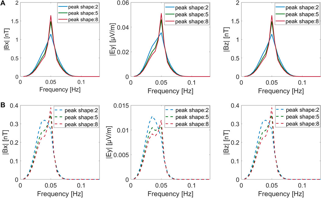
FIGURE 11. Electromagnetic field spectrum for peak shape parameters γ_S = 2, 5, and 8 at the sea surface (A) and seafloor (B).

The electromagnetic fields induced by mixed ocean waves

In some cases, the realistic ocean waves are mixed with wind waves and swell, called mixed ocean waves. The former refers to wind waves in equilibrium with the local wind, while the latter is defined as the swell waves generated elsewhere and not significantly affected by the local wind at that time (Hwang et al., 2012; Garcia-Gabin, 2015).

In order to describe complicated sea states due to the coexistence of wind waves and ocean swell, a double-peaked spectrum is proposed by combining the wind wave system and the swell system (Guedes Soares, 1984, 1991; Rossi et al., 2021). Ochi and Hubble (1976) presented a double-peaked spectrum as a combination of two gamma distributions as follows:

$S\left(\omega \right)=\frac{1}{4}{\displaystyle \sum _{j=1}^2}\frac{{\left(\frac{4{\lambda }_j+1}{4}{\omega }_{pj}^4\right)}^{{\lambda }_j}}{\mathrm{\Gamma }\left({\lambda }_j\right)}\frac{H_{sj}^2}{{\omega }^{4{\lambda }_j+1}}\exp \left[-\left(\frac{4{\lambda }_j+1}{4}\right){\left(\frac{{\omega }_{pj}}{\omega }\right)}^4\right](38)$

with

$\mathrm{\Gamma }\left({\lambda }_j\right)={\int }_0^{+\infty }{s}^{{\lambda }_j-1}{e}^{-s}ds\left(s>0\right),(39)$

where $H_{sj}$, ${\omega }_{pj}$, and ${\lambda }_j$ $\left(j=\mathrm{1,2}\right)$ are the significant wave height, angular peak frequency, and spectral shape factor, respectively, for low- and high-frequency parts (known as swell and wind–sea components, respectively). The parameters $H_{s1}$, $H_{s2}$, ${\omega }_{p1}$, ${\omega }_{p2}$, ${\lambda }_1$, and ${\lambda }_2$ involved in Eq. 38 are determined for the appropriate initial values.

Due to the difference in the effect caused by the wind waves and swell, the spectrum of the mixed ocean waves can be divided into three types: the strong wind and weak swell type, weak wind and strong swell type, and equivalent wind and swell type. The classification of the three types can be determined by the $0^{th}$ spectral moment of the wind waves and swell, which are defined as $S{m}_1$ and $S{m}_2$, respectively (Cai et al., 2007):

$S{m}_1=\frac{1}{4}{\int }_0^{\infty }\frac{{\left(\frac{4{\lambda }_1+1}{4}{\omega }_{p1}^4\right)}^{{\lambda }_1}}{\mathrm{\Gamma }\left({\lambda }_1\right)}\frac{H_{s1}^2}{{\omega }^{4{\lambda }_1+1}}\exp \left[-\left(\frac{4{\lambda }_1+1}{4}\right){\left(\frac{{\omega }_{p1}}{\omega }\right)}^4\right]d\omega ,(40)$

$S{m}_2=\frac{1}{4}{\int }_0^{\infty }\frac{{\left(\frac{4{\lambda }_2+1}{4}{\omega }_{p2}^4\right)}^{{\lambda }_2}}{\mathrm{\Gamma }\left({\lambda }_2\right)}\frac{H_{s2}^2}{{\omega }^{4{\lambda }_2+1}}\exp \left[-\left(\frac{4{\lambda }_2+1}{4}\right){\left(\frac{{\omega }_{p2}}{\omega }\right)}^4\right]d\omega .(41)$

Table 2 shows the parameters of the mixed ocean waves. Figure 12 shows that the energy in the spectrum of weak wind and strong swell type is usually concentrated at low frequencies, but the energy in the spectrum of the strong wind and weak swell type is usually concentrated at high frequencies. The energy distribution is more balanced in the spectrum of the equivalent wind and swell type.

TABLE 2

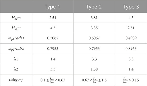
TABLE 2. Parameters of mixed ocean waves; type 1: strong wind and weak swell type; type 2: equivalent wind and swell type; and type 3: weak wind and strong swell type.

FIGURE 12

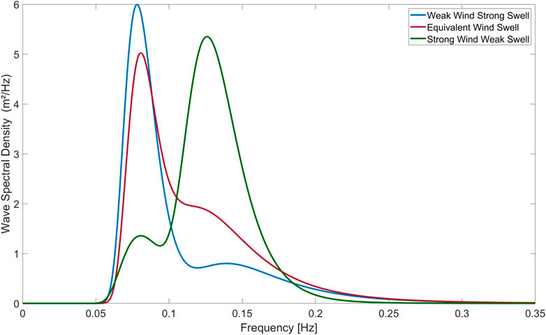
FIGURE 12. Double-peaked spectrum of the weak wind and strong swell type (the blue line), the equivalent wind and swell type (red line), and the strong wind and weak swell type (the green line).

The electromagnetic fields induced by three types of mixed ocean waves are shown in Figure 13. From Figure 13, we can see that 1) the three-type mixed wave spectrum can be easily recognized by the x- and z-components of the induced magnetic intensity strength spectrum observed at the sea surface (Figure 13A); 2) due to the high-frequency filtering effect of the ocean, the electromagnetic field spectra at the seafloor (Figure 13B) mainly retain the low-frequency information on the wave spectrum and may not reflect the realistic spectrum of the mixed ocean waves.

FIGURE 13

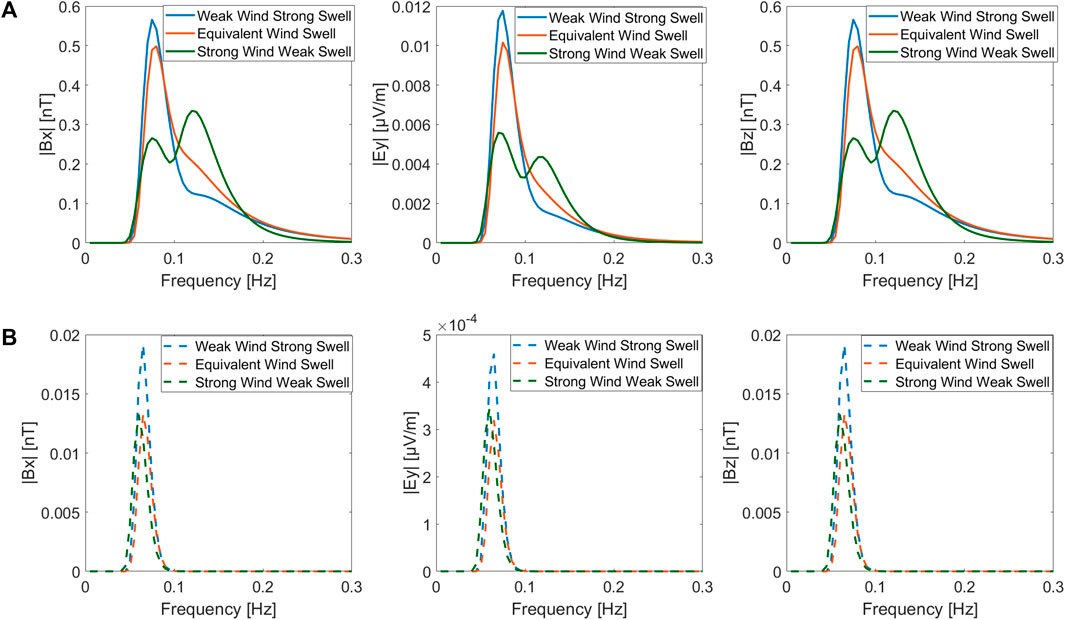
FIGURE 13. Electromagnetic fields induced by three types of mixed ocean waves at the sea surface (A) and seafloor (B).

Conclusion

In this paper, we presented a finite difference algorithm for simulating ocean wave-induced electromagnetic fields with varying seawater conductivity. Our method allows us to simulate and investigate the influence of arbitrary variation in seawater conductivity on wave-induced electromagnetic fields. Our numerical examples show that seawater conductivity has a significant effect on wave-induced electromagnetic fields. We also investigated the effects of the thermocline on wave-induced electromagnetic responses at different latitudes and seasons. We observed the maximum amplitude of induced electromagnetic fields in the mid-latitude regions, while we observed the minimum amplitude of induced electromagnetic fields in the polar regions. This is mainly influenced by both the geomagnetic field and temperature of the thermocline at different latitudes. Furthermore, in mid-latitude regions, the thermocline conductivity exhibits seasonal variations, with a greater decrease during summer than that during winter, leading to a larger induced electromagnetic field. The latitude and seasonal variations in the geomagnetic field and seawater conductivity are crucial for the accurate simulation of ocean wave-induced electromagnetic fields.

Moreover, we simulate the electromagnetic field spectra for wind waves, ocean swell, and mixed ocean waves in the inhomogeneous ocean. We find that the energy of the wind wave-induced electromagnetic field is predominantly concentrated in the high-frequency band, while the energy of the swell wave-induced electromagnetic field is mainly concentrated in the low-frequency band. Additionally, we simulate three types of mixed wave-induced electromagnetic fields based on the combination of wind and swell strengths, and analyze their characteristics.

Data availability statement

The original contributions presented in the study are included in the article/Supplementary Material; further inquiries can be directed to the corresponding author.

Author contributions

JG implemented the algorithms, drew the figures, and wrote the manuscript. YL led the research, supervised the study, and edited the manuscript. All authors contributed to the article and approved the submitted version.

Funding

This work was supported by the National Science Foundation of China (91958210 and U2241201).

Acknowledgments

The authors thank Ji Cai for helping in manuscript editing.

Conflict of interest

YL is a adjunct professor of the National Engineering Research Center of Offshore Oil and Gas Exploration.

The remaining author declares that the research was conducted in the absence of any commercial or financial relationships that could be construed as a potential conflict of interest.

Publisher’s note

All claims expressed in this article are solely those of the authors and do not necessarily represent those of their affiliated organizations, or those of the publisher, the editors, and the reviewers. Any product that may be evaluated in this article, or claim that may be made by its manufacturer, is not guaranteed or endorsed by the publisher.

References

Ailliot, P., Maisondieu, C., and Monbet, V. (2013). Dynamical partitioning of directional ocean wave spectra. Probabilistic Eng. Mech. 33, 95–102. doi:10.1016/j.probengmech.2013.03.002

CrossRef Full Text | Google Scholar

Cai, F., Liu, Q., and Miu, Q. (2007). Study on numerical simulation of bi-spectrum wave. Shanghai, China: The Chinese Society Of Naval Architects And Marine Engineers, 512–515.

Google Scholar

Chave, A. D., and Luther, D. S. (1990). Low-frequency, motionally induced electromagnetic fields in the ocean: 1. Theory. J. Geophys. Res. 95, 7185. doi:10.1029/JC095iC05p07185

CrossRef Full Text | Google Scholar

Chave, A. D. (1983). On the theory of electromagnetic induction in the Earth by ocean currents. J. Geophys. Res. Solid Earth 88, 3531–3542. doi:10.1029/JB088iB04p03531

CrossRef Full Text | Google Scholar

Cieutat, J.-M., Gonzato, J.-Ch., and Guitton, P. “A general ocean waves model for ship design,” in Proceedings of the Conference: Virtual Concept, Biarritz, France, November 2003.

Google Scholar

Cox, C., Kroll, N., Pistek, P., and Watson, K. (1978). Electromagnetic fluctuations induced by wind waves on the deep-sea floor. J. Geophys. Res. 83, 431. doi:10.1029/JC083iC01p00431

CrossRef Full Text | Google Scholar

Crews, A., and Futterman, J. (1962). Geomagnetic micropulsations due to the motion of ocean waves. J. Geophys. Res. 67, 299–306. doi:10.1029/JZ067i001p00299

CrossRef Full Text | Google Scholar

Fofonoff, N. P., and Millard, R. C. (1983). Algorithms for the computation of fundamental properties of seawater. Paris, France: UNESCO. doi:10.25607/OBP-1450

CrossRef Full Text | Google Scholar

Fraser, D. C. (1966). The magnetic fields of ocean waves. Geophys. J. R. Astronomical Soc. 11, 507–517. doi:10.1111/j.1365-246X.1966.tb03162.x

CrossRef Full Text | Google Scholar

Gao, X., Ma, X., Ma, Y., Huang, X., Zheng, Z., and Dong, G. (2022). Spectral characteristics of swell-dominated seas with in situ measurements in the coastal seas of Peru and Sri Lanka. J. Atmos. Ocean. Technol. 39, 755–770. doi:10.1175/JTECH-D-21-0143.1

CrossRef Full Text | Google Scholar

Garcia-Gabin, W. (2015). Wave bimodal spectrum based on swell and wind-sea components. IFAC-PapersOnLine 48, 223–228. doi:10.1016/j.ifacol.2015.10.284

CrossRef Full Text | Google Scholar

Grainger, J. P., Sykulski, A. M., Jonathan, P., and Ewans, K. (2021). Estimating the parameters of ocean wave spectra. Ocean. Eng. 229, 108934. doi:10.1016/j.oceaneng.2021.108934

CrossRef Full Text | Google Scholar

Guedes Soares, C. (1991). On the occurrence of double peaked wave spectra. Ocean. Eng. 18, 167–171. doi:10.1016/0029-8018(91)90040-W

CrossRef Full Text | Google Scholar

Guedes Soares, C. (1984). Representation of double-peaked sea wave spectra. Ocean. Eng. 11, 185–207. doi:10.1016/0029-8018(84)90019-2

CrossRef Full Text | Google Scholar

Håland, E., Flekkøy, E. G., and Måløy, K. J. (2012). Vertical and horizontal components of the electric background field at the sea bottom. GEOPHYSICS 77, E1–E8. doi:10.1190/geo2011-0039.1

CrossRef Full Text | Google Scholar

Hasselmann, K., Barnett, T. P., Bouws, E., Carlson, H., Cartwright, D. E., Enke, K., et al. (1973). Hamburg, Germany: Deutches Hydrographisches Institut.Measurements of wind-wave growth and swell decay during the joint north sea wave project (JONSWAP)

Google Scholar

Hwang, P. A., Ocampo-Torres, F. J., and García-Nava, H. (2012). Wind Sea and swell separation of 1D wave spectrum by a spectrum integration method. J. Atmos. Ocean. Technol. 29, 116–128. doi:10.1175/JTECH-D-11-00075.1

CrossRef Full Text | Google Scholar

Irrgang, C., Saynisch, J., and Thomas, M. (2016). Impact of variable seawater conductivity on motional induction simulated with an ocean general circulation model. Ocean. Sci. 12, 129–136. doi:10.5194/os-12-129-2016

CrossRef Full Text | Google Scholar

Larsen, J. C. (1971). The electromagnetic field of long and intermediate water waves. J. Mar. Res. 29.

Google Scholar

Lilley, F. E. M., Hitchman, A. P., Milligan, P. R., and Pedersen, T. (2004a). Sea-surface observations of the magnetic signals of ocean swells. Geophys. J. Int. 159, 565–572. doi:10.1111/j.1365-246X.2004.02420.x

CrossRef Full Text | Google Scholar

Lilley, F. E. M., Ted), , and Weitemeyer, K. A. (2004b). Apparent aeromagnetic wavelengths of the magnetic signals of ocean swell. Explor. Geophys. 35, 137–141. doi:10.1071/EG04137

CrossRef Full Text | Google Scholar

Longuet-Higgins, M. S. (1962). The directional spectrum of ocean waves, and processes of wave generation. Proc. R. Soc. Lond. Ser. A, Math. Phys. Sci. 265, 286–315. doi:10.1098/rspa.1962.0010

CrossRef Full Text | Google Scholar

Lucas, C., and Guedes Soares, C. (2015). On the modelling of swell spectra. Ocean. Eng. 108, 749–759. doi:10.1016/j.oceaneng.2015.08.017

CrossRef Full Text | Google Scholar

Miles, T., Dosso, H. W., and Ng, T. P. (1977). An analogue model for studying magnetic variations induced by ocean waves. Phys. Earth Planet. Interiors 14, 137–142. doi:10.1016/0031-9201(77)90150-9

CrossRef Full Text | Google Scholar

Minami, T. (2017). Motional induction by tsunamis and ocean tides: 10 Years of progress. Surv. Geophys. 38, 1097–1132. doi:10.1007/s10712-017-9417-3

CrossRef Full Text | Google Scholar

Minami, T., Schnepf, N. R., and Toh, H. (2021). Tsunami-generated magnetic fields have primary and secondary arrivals like seismic waves. Sci. Rep. 11, 2287. doi:10.1038/s41598-021-81820-5

PubMed Abstract | CrossRef Full Text | Google Scholar

Minami, T., and Toh, H. (2013). Two-dimensional simulations of the tsunami dynamo effect using the finite element method. Geophys. Res. Lett. 40, 4560–4564. doi:10.1002/grl.50823

CrossRef Full Text | Google Scholar

Nielsen, U. D., and Dietz, J. (2020). Ocean wave spectrum estimation using measured vessel motions from an in-service container ship. Mar. Struct. 69, 102682. doi:10.1016/j.marstruc.2019.102682

CrossRef Full Text | Google Scholar

Ochadlick, A. R. (1989). Measurements of the magnetic fluctuations associated with ocean swell compared with Weaver’s Theory. J. Geophys. Res. 94 (16), 16237–16242. doi:10.1029/JC094iC11p16237

CrossRef Full Text | Google Scholar

Ochi, M. K., and Hubble, E. N. (1976). Six-parameter wave spectra. Coast. Eng. Proc. 1, 17. doi:10.9753/icce.v15.17

CrossRef Full Text | Google Scholar

Rasool, S., Muttaqi, K. M., and Sutanto, D. (2021). Modelling Ocean waves and an investigation of ocean wave spectra for the wave-to-wire model of energy harvesting. Eng. Proc. 12, 51. doi:10.3390/engproc2021012051

CrossRef Full Text | Google Scholar

Rossi, G. B., Crenna, F., Berardengo, M., Piscopo, V., and Scamardella, A. (2021). Investigation on spectrum estimation methods for bimodal sea state conditions. Sensors (Basel) 21, 2995. doi:10.3390/s21092995

PubMed Abstract | CrossRef Full Text | Google Scholar

Ryabkova, M., Karaev, V., Guo, J., and Titchenko, Yu. (2019). A review of wave spectrum models as applied to the problem of radar probing of the sea surface. J. Geophys. Res. Oceans 124, 7104–7134. doi:10.1029/2018JC014804

CrossRef Full Text | Google Scholar

Semkin, S. V., and Smagin, V. P. (2012). The effect of self-induction on magnetic field generated by sea surface waves. Izv. Atmos. Ocean. Phys. 48, 207–213. doi:10.1134/S0001433812020119

CrossRef Full Text | Google Scholar

Shimizu, H., and Utada, H. (2015). Motional magnetotellurics by long oceanic waves. Geophys. J. Int. 201, 390–405. doi:10.1093/gji/ggv030

CrossRef Full Text | Google Scholar

Techet, A. H. (2005). 13.42 design principles for ocean vehicles. https://ocw.mit.edu/courses/2-22-design-principles-for-ocean-vehicles-13-42-spring-2005/fea036f3255fa4824279668c7ff8c6cd_r1_lti.pdf.

Google Scholar

Tyler, R. H., Boyer, T. P., Minami, T., Zweng, M. M., and Reagan, J. R. (2017). Electrical conductivity of the global ocean. Earth, Planets Space 69, 156. doi:10.1186/s40623-017-0739-7

PubMed Abstract | CrossRef Full Text | Google Scholar

Weaver, J. T. (1965). Magnetic variations associated with ocean waves and swell. J. Geophys. Res. 70, 1921–1929. doi:10.1029/JZ070i008p01921

CrossRef Full Text | Google Scholar

Yaakobi, O., Zilman, G., and Miloh, T. (2011). Detection of the electromagnetic field induced by the wake of a ship moving in a moderate sea state of finite depth. J. Eng. Math. 70, 17–27. doi:10.1007/s10665-010-9410-z

CrossRef Full Text | Google Scholar

Zhan, Y., and Pan, X. (2019). Propagation characteristics of electromagnetic wave in seawater channel for submerged buoy. J. Comput. Commun. 7, 72–81. doi:10.4236/jcc.2019.710007

CrossRef Full Text | Google Scholar

Zheng, Z., Fu, Y., Liu, K., Xiao, R., Wang, X., and Shi, H. (2018). Three-stage vertical distribution of seawater conductivity. Sci. Rep. 8, 9916. doi:10.1038/s41598-018-27931-y

PubMed Abstract | CrossRef Full Text | Google Scholar

Zhu, X., and Xia, M. (2014). Magnetic field induced by wake of moving body in wind waves (Invited Paper). PIER 149, 109–118. doi:10.2528/PIER14070706

CrossRef Full Text | Google Scholar