A general forward solver for 3D CSEMs with multitype sources and operating environments

1 Introduction

Controlled-source electromagnetic methods (CSEMs) are a group of geophysical exploration methods that transmit an electromagnetic (EM) signal using an artificial source (Goldstein and Strangway, 1975; Zonge and Hughes, 1991; Constable and Srnka, 2007; Di et al., 2020). CSEMs exhibit various classifications based on different factors, such as the type of source (e.g., wire, loop, electric, and magnetic dipole) and the operating environment (e.g., land, marine, airborne, and borehole), including marine frequency-/time-domain EM methods (mFD/TDCSEMs) (Edwards, 2005; Um and Alumbaugh, 2007; Connell and Key, 2013), long- and short-offset transient EM methods (L/SOTEMs) (Commer and Newman, 2004; Xue, 2018), controlled-source audio-frequency magnetotelluric (CSAMT) methods (Weng et al., 2012; Yang and Oldenburg, 2016), and land/airborne transient EM methods (TEMs) (Yin et al., 2016; Li et al., 2018; Zhang et al., 2018). By examining and analyzing the distribution patterns of the EM fields of CSEMs associated with variations in the resistivity of underground media, geophysicists can explore mineral and hydrocarbon resources (Hu et al., 2013; Streich, 2016; Schaller et al., 2018; Castillo-Reyes et al., 2022) and address geological and environmental engineering challenges (Everett, 2009; Chave et al., 2017; Malovichko et al., 2019; Castillo-Reyes et al., 2022).

Forward modeling is an effective way to study the EM field laws of CSEMs, and it is also the premise and basis of inversion methods (Avdeev, 2005; Börner, 2010). Over the past decades, innovations in numerical calculations have driven remarkable progress in the three-dimensional (3D) forward modeling of CSEMs, achieving successful breakthroughs (Constable, 2010; Ansari and Farquharson, 2013; Börner et al., 2015; Oldenburg et al., 2020; Werthmüller et al., 2021). The common methods used for developing the 3D forward modeling of CSEMs include finite element techniques (Tonti, 2002; Um et al., 2012; Cai et al., 2014; Rochlitz et al., 2019; Castillo-Reyes et al., 2022), finite volume methods (Haber and Ascher, 2001; Ren et al., 2017; Peng et al., 2018), finite difference methods (Newman and Alumbaugh, 1995; Weiland, 1996; Li et al., 2022), integral equation techniques (Hursán and Zhdanov, 2002; Tang et al., 2018), and spectral element methods (Huang et al., 2019; Xu and Tang, 2022). Furthermore, numerous scholars have dedicated research efforts to enhance the efficiency of numerical solutions in 3D forward modeling for CSEMs. They have employed parallel programming and numerical computation platforms to accelerate the computation speed (Unno et al., 2012; Koldan et al., 2014; Castillo-Reyes et al., 2018; Castillo-Reyes et al., 2019; Castillo-Reyes et al., 2022; Liu et al., 2023).

By employing forward modeling of different CSEMs, geophysical companies, scientific institutions, and individuals can compare the characteristics of EM responses and determine which CSEM offers the strongest resolution for specific geological targets while optimizing the survey parameter design before conducting field studies. However, the majority of forward modeling codes have been developed by various scientific institutions using different programming languages and focusing on a single CSEM with a specific source type and operating environment. The code of each CSEM is based on different essential mathematical procedures and utilizes different parameters for forward solutions, such as grids, interpolations, stations, numerical solution methods, and staggering schemes. These variations in parameterization can introduce biases during resolution analysis. Meanwhile, the expensive cost of secondary development for those codes poses practical challenges. The application effectiveness of a CSEM is influenced by the complexity and risk associated with the forward modeling theory. Technology implementation is the underlying support for practical applications. Therefore, it is necessary to decouple practical applications and concrete mathematical technology to advance geophysical science.

To simplify the forward theory and analyze the EM characteristics of different CSEMs for the same targets using the same parameters of the forward solution and mathematical procedures, we integrated forward modeling technologies and developed a forward solver for CSEMs with multitype sources and operating environments. In this study, our approach involves decomposing the total EM fields into the primary/background fields and secondary/scattered fields. This decomposition helps eliminate the singularity of the EM fields near the source. The primary field can be calculated by using the frequency-domain (FD) and full-space Green’s function of the source in a one-dimensional (1D) layered medium. The secondary field can be obtained by solving an FD vector Helmholtz equation for the scattered electric field, which is the reusable design part of the forward modeling for CSEMs. The procedure is the same regardless of the source type used to generate this field and regardless of operating in land, marine, airborne, or borehole environments.

On the other hand, any source type can be viewed as a combination of electric dipoles (EDs) or magnetic dipoles (MDs), each of which can be further decomposed into two horizontal EDs or MDs along the x and y directions, and one vertical ED or MD along the z direction. Thus, the focus of 3D forward modeling of CSEMs is reduced to solving EM fields for the background medium for ED or MD sources. By employing this approach, we can analyze the EM characteristics of different CSEMs using the same parameters for the forward solution, thus enhancing the comparability and understanding of the results.

The forward solver defines the overall structures and the main responsibilities of each module, thereby reducing the difficulty of solving EM fields of CSEMs and simplifying the implementation process of the theory. By avoiding the need to repeatedly construct the underlying mathematical logic, this approach enables geophysicists to focus on their unique application innovation. This paper first gives a brief overview of the mathematical methodology for 3D FD modeling of CSEMs. Once the FD EM fields have been calculated, the time-domain (TD) response can be obtained using the cosine/sine transformation. Then, the accuracy of the solver is verified by comparing the 3D modeling results with reference results obtained from 1D and 3D numerical solutions. Finally, we present two 3D modeling examples and discuss the effects of source shape and type on the EM fields of CSEMs over a 3D conductive Earth model.

2 Methodology

2.1 Maxwell’s equations

Assuming harmonic time dependence $e^{-\mathrm{i}\omega \mathrm{t}}$, Maxwell’s equations for the EM fields in the FD can be written as (Streich, 2009)

$\nabla \times \mathbf{E}=-\mathrm{i}\omega {\mu }_{\mathbf{0}}\mathbf{H},(1)$

$\nabla \times \mathbf{H}=\mathbf{J}+{\sigma }^{*}\mathbf{E},(2)$

where i² = −1, $\omega =2\pi f$ is the angular frequency, f is the frequency, E and H denote the total electric and magnetic fields, μ₀ within the Earth is assumed to be constant and set to that of free space, J is the source current distribution, ${\sigma }^{*}=\sigma +\mathrm{i}\omega \epsilon$ is the ohmic conduction term, σ is the electric conductivity, ε represents the air dielectric constant, and ${\sigma }^{*}\mathbf{E}$ describes the induced currents inside the Earth. According to Eqs 1, 2, the expression of the FD vector Helmholtz equation for the scattered electric field is as follows (Alumbaugh et al., 1996):

$\nabla \times \nabla \times {\mathbf{E}}^{\mathrm{s}}-k^2{\mathbf{E}}^{\mathrm{s}}=\left(k^2-k_p^2\right){\mathbf{E}}^{\mathrm{p}},(3)$

where $k^2=-\mathrm{i}\omega {\mu }_0\left(\sigma +\mathrm{i}\omega \epsilon \right)$, the superscripts “p” and “s” represent the primary and scattered fields, respectively, and E^s and E^p denote the scattered and primary electrical fields, respectively. Eq. 3 forms the basis of the presented modeling scheme and is well suited for simulations in CSEMs. Eq. 3 can overcome the difficulty of source description and the influence of source singularity on the numerical stability. Regardless of the type of source used to create the field, the procedure for calculating the scattered field remains the same. Then, we obtain the following PDE for the component $\widehat{\mathbf{i}}$:

$\frac{{\partial }^2{E}_y^{\mathrm{s}}}{\partial x\partial y}-\frac{{\partial }^2{E}_x^{\mathrm{s}}}{\partial y^2}-\frac{{\partial }^2{E}_x^{\mathrm{s}}}{\partial z^2}+\frac{{\partial }^2{E}_z^{\mathrm{s}}}{\partial x\partial z}-k^2{E}_x=\left(k^2-k_{\mathrm{p}}^2\right)E_x^{\mathrm{p}}.(4)$

2.2 The multitype source

In this paper, we adopt the ED or MD as the basic composition unit for any complex geometry source (Figure 1A). For example, the signal emission source of the LOTEM can be decomposed into many EDs (Figure 1B), and vector decomposition is applied to each ED (Figure 1C). The EM fields at any given position can be obtained by superimposing the EM fields generated by the ED component along the x, y, and z directions. Therefore, the primary objective of 3D forward modeling in CSEMs, regardless of the specific source type used, is to solve the electric field of an electric dipole or a magnetic dipole within the background models.

FIGURE 1

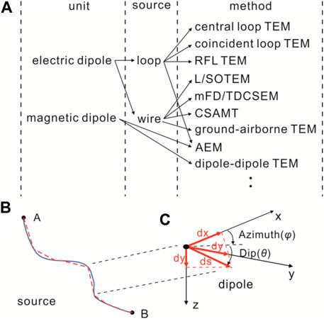
FIGURE 1. The electric or magnetic dipole is used as the unit of any CSEM sources (A). Finite-length wire source of LOTEM (B); A and B are the endpoints of the source, the solid line represents the real layout of the source, and the dotted line represents the source that is discretized by electric dipoles. Vector decomposition of an electric dipole (C).

2.3 Background models for primary fields

The primary field, as described by Weng et al. (2016), employs a virtual interface technique (Das and De Hoop, 1995) to solve the whole-space EM fields in a 1D layer model for different types of sources (Figure 2). These sources include vertical and horizontal electric dipoles (VED and HED) as well as vertical and horizontal magnetic dipoles (VMD and HMD).

FIGURE 2

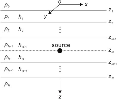
FIGURE 2. Homogeneous stratified medium with an EM transmitting source embedded in an intermediate layer. N is the number of layers, ρ₀, ρ₁, ρ₂, …, ρ_N are individual layer resistivities, h₀, h₁, h₂, …, h_N are layer thicknesses, and z₁, z₂, …, z_N denote the depth of the layer. The solid black circle denotes that the source is located at z_ls in the ls^th layer, and the dashed line denotes that a virtual interface is added at the source location parallel to the layer boundaries.

By separating the partial wave solutions of the Helmholtz equations into upward and downward waves within certain boundaries, the potentials for Green’s function are obtained. Starting from the source level, the amplitudes of the potentials in each layer are derived recursively based on the initial amplitudes. For different types of sources, only the initial terms that are associated with the transmitting sources need to be modified, and the kernel connected to the layered media remains the same. Hence, the aforementioned scheme can be easily applied to EM transmitting sources with slight modifications.

2.4 FD discretization

To calculate the scattered electric field in the medium, the geoelectric model is discretized by the cuboid cell (including the air layer) (Figure 3A), each denoted by a subscript (i, j, and k). The resistivity of each cell is represented by the symbol ρ (i, j, and k). i, j, and k represent the mesh indices in the x, y, and z directions, ranging from 1 to Nx, Ny, and Nz, respectively. Nx, Ny, and Nz denote the numbers of cells in the x, y, and z directions, respectively. Therefore, Eq. 4 can be discretized using the 3D staggered-grid finite-difference method, and the discretized expression is given in Eq. 5. The electric field components are defined on cell edges, while the magnetic field components naturally correspond to the cell faces (Figure 3B). The discrete finite difference equations of the $\widehat{\mathbf{j}}$ and $\widehat{\mathbf{k}}$ components are given in Appendix A.

$\begin{array}{c}\left\{[\frac{1}{\Delta x_i}\left(E_{y_{i+1,j+1/2,k}}^{\mathrm{s}}-E_{y_{i,j+1/2,k}}^{\mathrm{s}}\right)-\frac{1}{\Delta y_j}\left(E_{x_{i+1/2,j+1,k}}^{\mathrm{s}}-E_{x_{i+1/2,j,k}}^{\mathrm{s}}\right)\right]\left.-\left[\frac{1}{\Delta x_i}\left(E_{y_{i+1,j-1/2,k}}^{\mathrm{s}}-E_{y_{i,j-1/2,k}}^{\mathrm{s}}\right)-\frac{1}{\Delta y_{j-1}}\left(E_{x_{i+1/2,j,k}}^{\mathrm{s}}-E_{x_{i+1/2,j-1,k}}^{\mathrm{s}}\right)\right]\right\}\hfill \\ \cdot \frac{1}{\Delta {\overline{y}}_j}+\left\{[\frac{1}{\Delta x_i}\left(E_{z_{i+1,j,k+1/2}}^{\mathrm{s}}-E_{z_{i,j,k+1/2}}^{\mathrm{s}}\right)-\frac{1}{\Delta z_k}\left(E_{x_{i+1/2,j,k+1}}^{\mathrm{s}}-E_{x_{i+1/2,j,k}}^{\mathrm{s}}\right)\right]\left.-\left[\frac{1}{\Delta x_i}\left(E_{z_{i+1,j,k-1/2}}^{\mathrm{s}}-E_{z_{i,j,k-1/2}}^{\mathrm{s}}\right)-\frac{1}{\Delta z_{k-1}}\left(E_{x_{i+1/2,j,k}}^{\mathrm{s}}-E_{x_{i+1/2,j,k-1}}^{\mathrm{s}}\right)\right]\right\}\hfill \\ \cdot \frac{1}{\Delta {\overline{z}}_k}\begin{array}{l}+i\omega {\mu }_p{\widehat{y}}_p{E}_{x_{i+1/2,j,k}}^s\\ =-i\omega {\mu }_p\left({\widehat{y}}_{i+1/2,j,k}-{\widehat{y}}_p\right)E_{x_{i+1/2,j,k}}^p,\end{array}\hfill \end{array}(5)$

where $\widehat{y}=\sigma +i\omega \epsilon$, w = x, y, z, and l = i, j, k denote the length of the lth cell in the w direction, and $∆\overline{w_l}$ is the distance between the center of the lth and l1th cells in the w direction.

FIGURE 3

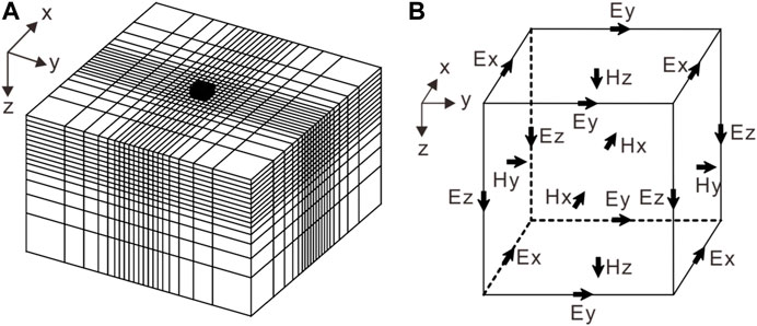
FIGURE 3. Staggered finite-difference grid for 3D CSEM forward modeling (A); the solid black cuboid indicates the survey area. The electric field components are defined on cell edges, and the magnetic field components can be defined naturally on the cell faces (B).

2.5 Preconditioning and numerical implementation

Equation 5 can be assembled into the following system:

${\mathbf{K}\mathbf{E}}^{\mathrm{s}}=\mathbf{b},(6)$

where K is the coefficient matrix, and b in the right-hand side consists of the dot products between the primary/background field and conductivity abnormalities, as well as the appropriate boundary conditions.

Generally, the coefficient matrix K for Eq. 6 is a large, sparse, and ill-conditioned matrix that is difficult to solve. To reduce the condition number of the coefficient matrix K, Eq. 6 can be written in the preprocessing form as follows:

$\left({\mathbf{K}\mathbf{M}}^{-1}\right)\cdot \mathbf{y}=\mathbf{b}.(7)$

Here, y = ME^s is the modified unknown vector, where the matrix M is called the (right-hand side) preprocessor, and the matrix KM^-1 is considered very close to the identity matrix. Once Eq. 7 is solved approximately, we can obtain E^s using the relationship between y and E^s. In this study, an incomplete Cholesky decomposition is used as the precondition to accelerate the convergence and improve the accuracy of the iterative solution. Eq. 7 can be solved by using the quasi-minimal residual method (QMR) (Mackie et al., 1994).

2.6 Boundary conditions and grid generation

Due to the significant difference between the solution region and the anomalous bodies, the secondary field will decay to zero at the boundary far from the anomalous body. As a result, we applied typical homogeneous Dirichlet’s boundary conditions. With n being the normal vector on the domain boundary δΩ, it is defined as:

$\mathbf{n}\times {\mathbf{E}}^{\mathbf{s}}=\mathbf{0}.(8)$

The grid generation is centered on the area of interest and is divided into finer grids near the anomaly bodies. As depicted in Figure 3A, the grid size gradually increases as the distance from the area of interest expands. The air layer is set to seven layers, with the uppermost layer having a thickness of 30 km. In our paper, the mini software CSEM mesh is used to generate the mesh, which was developed by teachers and students in our research group. It greatly reduces the cost of generating meshes.

2.7 Divergence correction

The divergence of the secondary electric field E^s is zero at any point except the source (Shen, 2003; Chen et al., 2011). Due to the accuracy of the numerical calculation, the divergence of E^s does not disappear during an iteration solution process which can be calculated using φ = $\nabla \cdot {\mathbf{E}}^{\mathrm{s}}$, considering the additional electrical field generated by the source φ. To calculate the additional electrical field, it is necessary to use the Neumann boundary conditions to solve the potential obtained by Poisson’s equation as follows:

$\nabla \cdot \nabla \psi =\phi .(9)$

When Eq. 6 is solved, the E^s values required for divergence correction can be expressed as follows:

${\mathbf{E}}_{\mathrm{c}\mathrm{o}\mathrm{r}\mathrm{r}\mathrm{e}\mathrm{c}\mathrm{t}}^{\mathrm{s}}={\mathbf{E}}_{\mathrm{o}\mathrm{l}\mathrm{d}}^{\mathrm{s}}-\nabla \psi ,(10)$

specifically, to satisfy the following equation:

$\nabla \cdot {\mathbf{E}}_{\mathrm{c}\mathrm{o}\mathrm{r}\mathrm{r}\mathrm{e}\mathrm{c}\mathrm{t}}^{\mathrm{s}}=\nabla \cdot {\mathbf{E}}_{\mathrm{o}\mathrm{l}\mathrm{d}}^{\mathrm{s}}-\nabla \cdot \nabla \psi =\phi -\phi =0.(11)$

The preconditioned conjugate gradient (PCG) algorithm is used to solve the divergence in Eq. 11. The iterative solution’s convergence rate is greatly improved, particularly at low frequencies (Smith, 1996a; Smith, 1996b).

2.8 FD EM field interpolation to receiver positions

Once E^s on the center of the grid edge is obtained by Eq. 6, the total electric field E can be estimated by adding a primary field E^p, that is,

$\mathbf{E}={\mathbf{E}}^{\mathrm{p}}+{\mathbf{E}}^{\mathrm{s}},(12)$

while the total magnetic field normal to the surface confined by the grid edge at the center can be approximated by Faraday’s law:

$-\mathrm{i}\omega \mathbf{B}=\nabla \times \mathbf{E},(13)$

from the estimated EM fields. Then, the EM fields at the position of interest can be interpolated by

$\mathbf{E}={\mathbf{L}}_e\mathbf{E}(14)$

and

$\mathbf{H}={\mathbf{L}}_{\mathrm{h}}\mathbf{H},(15)$

where L_e and L_h represent bilinear splines from the 3D grid nodes and edges, respectively, to the data sites.

2.9 TD EM responses

According to Weng et al. (2017), the TD EM signal h(t) through

$h\left(t\right)=\frac{1}{2\pi }{\int }_0^{\infty }I\left(\omega \right)H\left(\omega \right)e^{-\mathrm{i}\omega \mathrm{t}}\mathrm{d}\omega (16)$

is related to the FD response H(ω) from a source excited by current I(ω) over a conductive model; in the aforementioned equation, i² = −1, $\omega =2\pi f$ is the angular frequency, f is the frequency, and t is the time. If a step-off current is assumed, using the Euler formula, Eq. 16 can be further split into a sine transformation as follows:

$\mathrm{d}B/\mathrm{d}t={\mu }_0\mathrm{d}h/\mathrm{d}t=-{\mu }_0\frac{2}{\pi }{\int }_0^{\infty }\mathrm{I}\mathrm{m}\left[H\left(\omega \right)\right]\sin \left(\omega t\right)d\omega ,(17)$

where B is the magnetic flux density and Im [·] denotes the imaginary part of the FD EM fields. We sample the exact six points per decade FD data between 10^–3 Hz and 10⁸ Hz and obtain 67 frequencies (Liu et al., 2016). After obtaining the FD results, the TD EM responses for the step wave are calculated using Eq. 17. Based on the aforementioned theory, we have programmed a 3D forward modeling code using Fortran 90 for FD/TD CSEMs with multitype sources.

3 Model verification

To test the correctness and reliability of the aforementioned forward modeling solver for different types of sources, we initially design a 100 Ωm uniform half-space model for the airborne EM method (AEM) with a vertical magnetic dipole (VMD) source and a unit current (Liu and Yin, 2013). The flight altitude is set to 30 m, and the receiver is positioned 2 m away from the transmitter (Figure 4A). The model is divided into 20 × 20 × 25 prisms of dimension 10 m × 10 m × 10 m. The background model with 50 Ωm is used for computing the primary field. Figure 4B illustrates the comparisons between the 3D solution and the 1D results using a step-off current waveform. The results of the 3D solution agree well with the 1D result. The overall relative errors are less than 5%. Figure 4C shows a plot of the error versus iteration for the QMR solver for the uniform half-space model for the data with the four frequencies. We can clearly see that the QMR solver is stable and converges quickly to the values of 10^–7. We obtained similar results for the other models presented in this paper. The total memory required to solve this model was 73.24 MB. It took approximately 4.3 min per frequency to solve this model on a personal computer with an Intel^® Core™ i5-2320 processor and 8 GB memory.

FIGURE 4

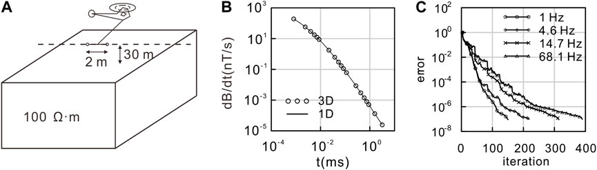
FIGURE 4. A uniform half-space is used to verify the numerical accuracy of 3D modeling for AEM with a VMD source. (A) 3D model. (B) Comparison of our 3D result against the 1D numerical solution for the TD EM fields (dB/dt). (C) Error curve of the QMR solver.

Second, we take the RFLTEM as an example, and a loop source with dimensions of 10 m × 10 m can be decomposed into many EDs. A 3D conductive body (50 m × 50 m × 50 m) of 20 Ωm is embedded in a two-layer Earth model in Ji et al. (2017) (Figure 5A). In the numerical simulation, the origin of the coordinate system is at the surface with the z-axis downward through the center of the abnormal body. The model is divided into 51 × 51 × 30 prisms of dimension 10 m × 10 m × 10 m. The FD EM fields are calculated at the measurement points Rx₁ and Rx₂ in Figure 5A. Then, dB_z/dt is obtained using Eq. (17), and it was normalized by the square of the single-turn receiving coil. The solution of the forward modeling solver agrees well with that in the study by Ji et al. (2017) (Figure 5B). These examples serve as strong evidence for the accuracy and reliability of our forward modeling code. Figure 5C shows a plot of the error versus iteration for the QMR solver for a two-layer model for the data with four frequencies. The error of the QMR solver converges quickly to the values of 10^–7. The total memory required to solve this model was 114.26 MB. It took approximately 6.8 min per frequency.

FIGURE 5

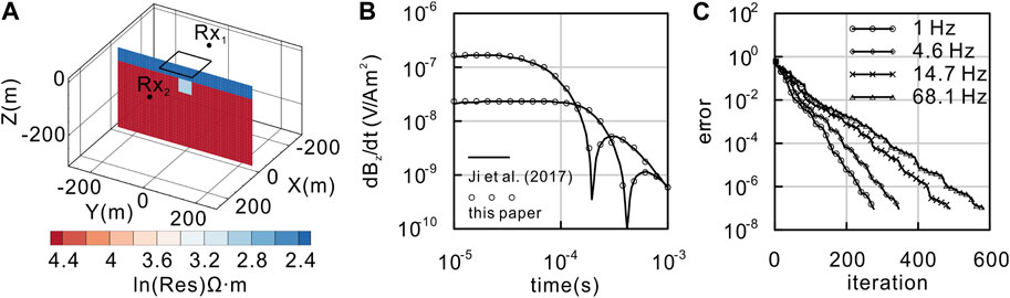
FIGURE 5. A two-layer model is used to verify the numerical accuracy of 3D modeling for the RFLTEM. (A) 3D model. (B) Comparison between the field solutions obtained in this paper and those of Ji et al. (2017) for the receiver positions denoted by Rx₁ (105, 0, 0) and Rx₂ (−155, 0, 0). (C) Error curve of the QMR solver.

4 Applications

4.1 The real and theoretical source

In real field surveys, surface obstacles and topography can preclude laying out the source in a theoretical shape such as a straight line, rectangle, or circle. The aforementioned scheme can segment a source with an arbitrarily complex shape into a large number of EDs and MDs. To illustrate this, we conducted a study taking the LOTEM and CSAMT as examples, focusing on the differences between the TD and FD EM fields for both straight and non-straight wire sources. We computed the TD and FD responses for the bent and straight wires. Both wires centered at (0, 0) have the same grounding points; the straight wires of 1 km have a 1 A current on the surface, and the bent wire is the real source consisting of 22 segments (Figure 6A). The 3D model of a 100 Ωm homogeneous half-space is shown in Figure 6B.

FIGURE 6

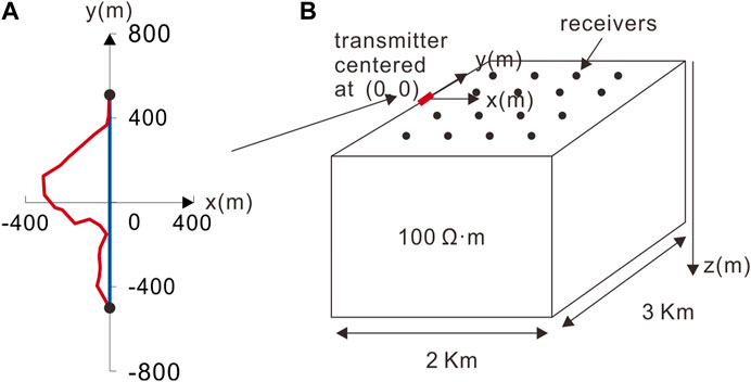
FIGURE 6. The survey geometry (A) and 3D model (B) are used for modeling a TD and FD CSEM survey. The red and blue lines indicate the real (bent) and theoretical (straight) wires, respectively. The red short line denotes the y-directed 1-km-long wire source.

In Figure 7, we display the TD magnetic field dB/dt for a bent wire compared to dB/dt for a straight wire at different times: 0.065 ms, 0.9 ms, 4 ms, and 10 ms. As time increases, the difference in dB/dt between the bent and straight wires decreases. dB/dt generated by the straight wire exhibits a symmetrical distribution around the source center and is concentrated near the surface (Figure 7A). At the early stage, there is a significant disparity in the dB/dt between the bent and straight wires (Figure 7C). Therefore, when analyzing early-time TEM data, it is crucial to consider the shape of the source. With a time delay, the center of dB/dt propagates downward and outward, and the strength of the field gradually decays. At the later stage, dB/dt continues to propagate and becomes more uniform, and the relative differences in dB/dt between the bent and straight wires are minimal (Figure 7C). Spatially, the closer the distance to the source, the greater the difference in dB/dt between the bent and straight wires. Conversely, the farther the distance to the source, the smaller the difference in dB/dt between the bent and straight wires. Therefore, when processing data of TEMs observed close to the source, such as the SOTEM, the source’s shape must be taken into account.

FIGURE 7

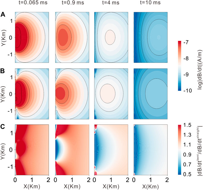
FIGURE 7. TD magnetic field dB/dt for the configuration shown in Figure 7 at different times of 0.065 ms, 0.9 ms, 4 ms, and 10 ms: (A) straight wire; (B) bent wire; (C) ratio difference between bent and straight wire fields.

Figure 8 shows the FD electric field component Ey for the bent wire relative to Ey for a straight wire at frequencies of 0.1 Hz, 2 Hz, 16 Hz, and 128 Hz. The relative differences in Ey between the bent and straight wires increase with increasing frequency and decrease with increasing distance from the source. At low frequencies, the difference in Ey between the bent and straight wires was very small, and it was mainly concentrated near the source and both sides along the emitting source direction. At high frequencies, the difference in Ey was most pronounced in the survey area. These results highlight the significant influence of the grounding points’ locations and the entire wire layout on the EM fields at these frequencies. Therefore, during the inversion of the high-frequency data from a wire source, such as the CSAMT, it is impossible to ignore the impact of the source’s shape on the measured data.

FIGURE 8

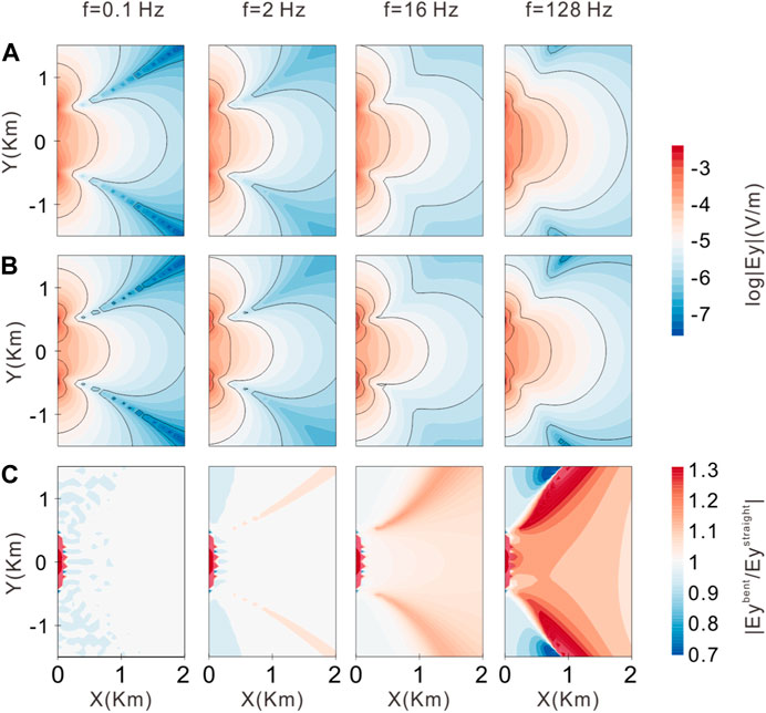
FIGURE 8. FD electric field Ey for the configuration shown in Figure 7 at frequencies of 0.1 Hz, 2 Hz, 16 Hz, and 128 Hz: (A) straight wire; (B) bent wire; (C) ratio of difference between the bent and straight wire fields.

The comparison between the TD and FD EM methods shows that the FD CSEM appears to be more significantly influenced by the entire wire layout than the TD CSEM. This difference can be attributed to the nature of the measurements. In the TD CSEMs, observations are made after the current is turned off, capturing the induced eddy field or secondary field. In this case, the shape of the emission source only affects the early data. On the other hand, in FD CSEMs, observations are made under the harmonic excitation of the source, representing the total field. The impact of the source’s shape on the field becomes more noticeable, particularly at higher frequencies. At low frequencies, the electric field resembles a potential field that occurs in the static limit. Here, the only factors affecting the electric field are the locations of the grounding points.

According to the aforementioned analysis, we suggest that the shape of the source must be considered for TD and FD CSEMs with a wire source during data processing and inversion. However, in regard to the influence of the source shape, we recommend TD CSEMs when processing data based on the theory of an ideal straight wire or electric dipole source for the same target.

4.2 Wire and loop sources

4.2.1 Model parameters

3D FD forward modeling and TD forward modeling of CSEMs with wire and loop sources were conducted using a conductive geological model in which a conductive tilted sheet is embedded in a uniform half-space with a strike of 525 m and two high- and low-resistivity bodies on the surface (Figure 9A). In the numerical simulation, the origin of the coordinate system was set at the center of the model at the ground, with the z-axis pointing downward. The model space is subdivided into 40 × 40 × 20 prisms of size 25 m × 25 m × 25 m. To ensure that Dirichlet’s boundary condition was satisfied, boundary cells in the five layers outside the model were expanded by a factor of 1.5 (Figures 9B–D). In the following solution calculation, all the parameters remained consistent for the 3D forward modeling of CSEMs with both loop and wire sources.

FIGURE 9

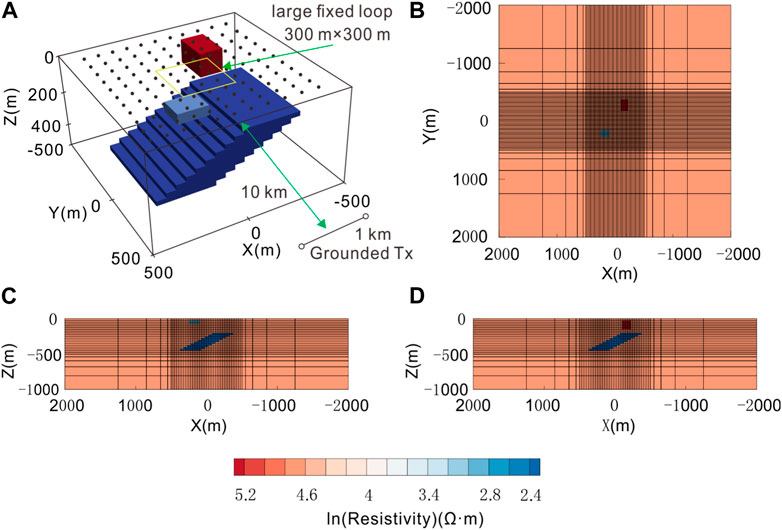
FIGURE 9. 3D conductive geological model and the grid used for the model. (A) View of the model used for 3D FD and TD forward modeling of CSEMs. The solid circles represent the position of the receivers. The yellow rectangle and the black line indicate the locations of the loop and wire sources, respectively; (B) plan view and rectangular mesh with Z = 120 m; (C) and (D) vertical sections and rectangular mesh with Y = −270 m and Y = 270 m, respectively.

4.2.2 TD CSEM with a loop source

In the TD CSEM, a larger rectangular fixed loop is commonly used as a source, encompassing the target area. The vertical TD magnetic field dB/dt is then measured both inside and outside the loop, simulating the RLFTEM. In this paper, the RLFTEM uses a fixed loop of dimension 300 m × 300 m with a 1 A current on the Earth’s surface (Figure 9A). Figure 10 shows the TD scattered field for two specific sections (Y = −270 m and Y = 270 m). According to Faraday’s law, the induced eddy currents within the anomalous body are excited when the transmitter switch is abruptly turned off, thus preventing the internal magnetic field of the anomalous body from weakening. At early times, the presence of surface resistive and conductive bodies distorts the induced eddy currents. With a time delay, the induced eddy currents diffuse downward and outward underground, leading to a gradual decay in the strength of the magnetic field. As observed from dB/dt, the RLFTEM has a higher sensitivity to conductive bodies than resistive anomalies.

FIGURE 10

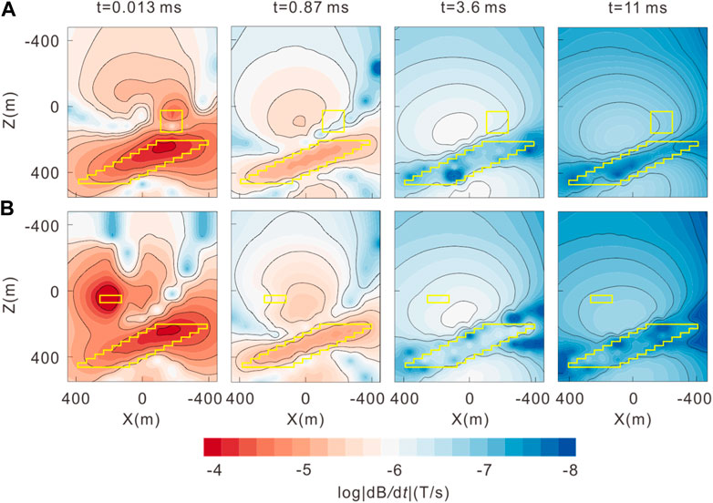
FIGURE 10. TD scattered field at t = 0.013 ms, 0.87 ms, 3.6 ms, and 11 ms: (A) Y = −270 m; (B) Y = 270 m. The yellow solid lines denote the position of the abnormal bodies. The black solid lines represent the contour line.

4.2.3 FD CSEM with a wire source

The wire source is generally used in land and marine CSEMs, such as the CSAMT, LOTEM, and GATEM, and the transmitter is a finite-length wire with complex geometry. In the numerical implementation, we take the CSAMT as an example. A finite-length wire with a length of 1 km and a current of 1 A was laid on the ground along the x direction as a signal source. The nearest measuring point is located at a distance of 10 km from the center of the source (Figure 9A). For the CSAMT, the electric field component Ex is generally used as the observed data, as in the wide-field EM method (He, 2010). The proposed forward modeling solver computes Ex in the whole space. The results of the calculation for two sections (Y = −270 m and Y = 270 m) are shown in Figure 11. The FD EM fields from the wire source are similar to those of a plane wave in the measurement area. Among these frequencies, f = 16 Hz is the most sensitive frequency for the tilted target body. The low-frequency data demonstrate a stronger resolution ability to the deep abnormal body. Moreover, high-frequency EM fields have higher energies and stronger abilities to resolve shallow abnormal bodies. However, due to their shorter wavelength and lower penetration, their overall ability to resolve deep anomalous bodies is relatively limited.

FIGURE 11

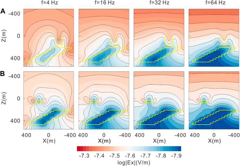
FIGURE 11. FD electric field at f = 4 Hz, 16 Hz, 32 Hz, and 64 Hz. (A) Y = −270 m; (B) Y = 270 m. The yellow solid lines denote the position of the abnormal bodies. The black solid lines represent the contour line.

The RFLTEM and CSAMT utilize loop and wire sources, representing the magnetic and electric sources, respectively. By comparing the forward results of the RFLTEM and CSAMT, we can see that both methods are sensitive to shallow conductive anomalies. However, in terms of resolving shallow resistive anomalies, the CSAMT demonstrates a better resolution than the RFLTEM. The observed data distortion, primarily caused by deep conductivity anomalies, is more pronounced in the CSAMT than in the RLFTEM. Furthermore, the resolution of the CSAMT is stronger than that of the RLFTEM for spatial information, such as the occurrence of deep tilted sheets.

Based on the aforementioned analysis, TD CSEMs with loop sources (central loop, coincident loop, and dipole–dipole) are recommended for detecting shallow conductivity anomalies due to their convenience and higher efficiency. On the other hand, for detecting deep anomalies, FD CSEMs with a wire source are sensitive to both resistive and conductive abnormal bodies. The 3D forward modeling solver of CSEMs provides valuable assistance to geophysicists in selecting the most suitable exploration method based on the same forward modeling parameters.

5 Conclusion

In this paper, we have considered the significant commonalities of 3D forward modeling for TD and FD CSEMs with different types of sources and operating environments and developed a general forward solver. Using the same format, the source term of CSEMs is imposed on the right-hand term of an FD vector Helmholtz equation for the scattered electric field. Any complex geometry source can be decomposed into EDs or MDs used as the basic composition unit, each of which can be further decomposed into two horizontal EDs or MDs along the x and y directions and one vertical ED or MD along the z direction. Through this solver, geophysicists can compare the EM field characteristics of different CSEMs for the specific geological targets using the same parameters of the forward solution.

Based on the numerical experimental results of the real and theoretical sources, we suggest that the shape of the source must be considered for TD and FD CSEMs. According to the numerical experiment results of wire and loop sources, we recommend TD CSEMs with the loop source for detecting shallow conductivity abnormal bodies. Moreover, we recommend FD CSEMs with a wire source for detecting deep anomalies.

The solver proposed in this paper leads us to clearly define the basic target objects and methods needed to solve the 3D TD and FD forward problem of the general CSEMs. In the future, we need to further optimize the code computational efficiency, improve the speed of program running, reduce the memory requirements, and lay the foundation for the geophysical interpretation of TD and FD EM data.

Data availability statement

The original contributions presented in the study are included in the article/Supplementary Material; further inquiries can be directed to the corresponding author.

Author contributions

DL implemented the algorithms and wrote the manuscript. YL and ZW conceived the idea of the algorithm, supervised the study, performed the analyses, and edited the manuscript. LJ helped in processing the data and prepared the figures. All authors contributed to the article and approved the submitted version.

Funding

This research was supported by the Natural Science Foundation of Jilin Province, China (Grant Number YDZJ202301ZYTS222) and Jilin Province Education Department Science and Technology Research Project (Grant Number JJKH20230347KJ).

Acknowledgments

Thanks are given to the two reviewers and editors for their helpful suggestions and for improving the manuscript. We would like to thank Prof. Aihua Weng, who modified the whole paper.

Conflict of interest

The authors declare that the research was conducted in the absence of any commercial or financial relationships that could be construed as a potential conflict of interest.

Publisher’s note

All claims expressed in this article are solely those of the authors and do not necessarily represent those of their affiliated organizations, or those of the publisher, the editors, and the reviewers. Any product that may be evaluated in this article, or claim that may be made by its manufacturer, is not guaranteed or endorsed by the publisher.

References

Alumbaugh, D. L., Newman, G. A., Prevost, L., and Shadid, J. N. (1996). Three-dimensional wideband electromagnetic modeling on massively parallel computers. Radio Sci. 31 (1), 1–23. doi:10.1029/95RS02815

CrossRef Full Text | Google Scholar

Ansari, S., and Farquharson, C. G. (2013). 3D finite-element forward modeling of electromagnetic data using vector and scalar potentials and unstructured grids. Geophysics 79 (4), E149–E165. doi:10.1190/GEO2013-0172.1

CrossRef Full Text | Google Scholar

Avdeev, D. B. (2005). Three-dimensional electromagnetic modelling and inversion from theory to application. Surv. Geophys. 26 (6), 767–799. doi:10.1007/s10712-005-1836-x

CrossRef Full Text | Google Scholar

Börner, R. U., Ernst, O. G., and Güttel, S. (2015). Three-dimensional transient electromagnetic modelling using Rational Krylov methods. Geophys. J. Int. 202 (3), 2025–2043. doi:10.1093/gji/ggv224

CrossRef Full Text | Google Scholar

Börner, R. U. (2010). Numerical modelling in geo-electromagnetics: Advances and challenges. Surv. Geophys. 31 (2), 225–245. doi:10.1007/s10712-009-9087-x

CrossRef Full Text | Google Scholar

Cai, H., Xiong, B., Han, M., and Zhdanov, M. (2014). 3D controlled-source electromagnetic modeling in anisotropic medium using edge-based finite element method. Comput. Geosciences 73, 164–176. doi:10.1016/j.cageo.2014.09.008

CrossRef Full Text | Google Scholar

Castillo-Reyes, O., Amor-Martin, A., Botella, A., Anquez, P., and García-Castillo, L. E. (2022). Tailored meshing for parallel 3D electromagnetic modeling using high-order edge elements. J. Comput. Sci. 63, 101813. doi:10.1016/j.jocs.2022.101813

CrossRef Full Text | Google Scholar

Castillo-Reyes, O., de la Puente, J., and Cela, J. M. (2022). HPC geophysical electromagnetics: A synthetic vti model with complex bathymetry. Energies 15 (4), 1272. doi:10.3390/en15041272

CrossRef Full Text | Google Scholar

Castillo-Reyes, O., de la Puente, J., and Cela, J. M. (2018). Petgem: A parallel code for 3D CSEM forward modeling using edge finite elements. Comput. Geosciences 119, 123–136. doi:10.1016/j.cageo.2018.07.005

CrossRef Full Text | Google Scholar

Castillo-Reyes, O., de la Puente, J., García-Castillo, L. E., and Cela, J. M. (2019). Parallel 3-D marine controlled-source electromagnetic modelling using high-order tetrahedral Nédélec elements. Geophys. J. Int. 219 (219), 39–65. doi:10.1093/gji/ggz285

CrossRef Full Text | Google Scholar

Castillo-Reyes, O., Modesto, D., Queralt, P., Marcuello, A., Ledo, J., Amor-Martin, A., et al. (2022). 3D magnetotelluric modeling using high-order tetrahedral Nédélec elements on massively parallel computing platforms. Comput. Geosciences 160, 105030. doi:10.1016/j.cageo.2021.105030

CrossRef Full Text | Google Scholar

Castillo-Reyes, O., Queralt, P., Marcuello, A., and Ledo, J. (2022). Land CSEM simulations and experimental test using metallic casing in a geothermal exploration context: Vallès basin (NE Spain) case study. IEEE Trans. Geoscience Remote Sens. 60, 1–13. doi:10.1109/TGRS.2021.3069042

CrossRef Full Text | Google Scholar

Chave, A. D., Everett, M. E., Mattsson, J., Boon, J., and Midgley, J. (2017). On the physics of frequency-domain controlled source electromagnetics in shallow water. 1: Isotropic conductivity. Geophys. J. Int. 208 (2), 1026–1042. doi:10.1093/gji/ggw435

CrossRef Full Text | Google Scholar

Chen, H., Deng, J. Z., Tan, H. D., and Yang, H. Y. (2011). Study on divergence correction method in three-dimensional magnetotelluric modeling with staggered-grid finite difference method. Chin. J. Geophys. (in Chinese) 54 (6), 1649–1659. doi:10.3969/j.issn.0001-5733.2011.06.025

CrossRef Full Text | Google Scholar

Commer, M., and Newman, G. (2004). A parallel finite-difference approach for 3D transient electromagnetic modeling with galvanic sources. Geophysics 69 (5), 1192–1202. doi:10.1190/1.1801936

CrossRef Full Text | Google Scholar

Connell, D., and Key, K. (2013). A numerical comparison of time and frequency-domain marine electromagnetic methods for hydrocarbon exploration in shallow water. Geophysical Prospecting 61 (1), 187–199. doi:10.1111/j.1365-2478.2012.01037.x

CrossRef Full Text | Google Scholar

Constable, S., and Srnka, L. J. (2007). An introduction to marine controlled-source electromagnetic methods for hydrocarbon exploration. Geophysics 72 (2), WA3–WA12. doi:10.1190/1.2432483

CrossRef Full Text | Google Scholar

Constable, S. (2010). Ten years of marine CSEM for hydrocarbon exploration. Geophysics 75 (5), 75A67–75A81. doi:10.1190/1.3483451

CrossRef Full Text | Google Scholar

Das, U. C., and De Hoop, A. T. (1995). Efficient computation of apparent resistivity curves for depth profiling of a layered Earth. Geophysics 60 (6), 1691–1697. doi:10.1190/1.1443901

CrossRef Full Text | Google Scholar

Di, Q., Xue, G., Yin, C., and Li, X. (2020). New methods of controlled-source electromagnetic detection in China. Science China Earth Sciences 63 (9), 1268–1277. doi:10.1007/s11430-019-9583-9

CrossRef Full Text | Google Scholar

Edwards, N. (2005). Marine controlled source electromagnetics: Principles, methodologies, future commercial applications. Surveys in Geophysics 26 (6), 675–700. doi:10.1007/s10712-005-1830-3

CrossRef Full Text | Google Scholar

Everett, M. E. (2009). Transient electromagnetic response of a loop source over a rough geological medium. Geophysical Journal International 177 (2), 421–429. doi:10.1111/j.1365-246X.2008.04011.x

CrossRef Full Text | Google Scholar

Goldstein, M. A., and Strangway, D. W. (1975). Audio-frequency magnetotellurics with a grounded electric dipole source. Geophysics 40 (4), 669–683. doi:10.1190/1.1440558

CrossRef Full Text | Google Scholar

Haber, E., and Ascher, U. M. (2001). Fast finite volume simulation of 3D electromagnetic problems with highly discontinuous coefficients. SIAM Journal of Scientific Computing 22 (6), 1943–1961. doi:10.1137/S1064827599360741

CrossRef Full Text | Google Scholar

He, J. S., Yang, Y., Di-quan, L., and Jing-bo, W. (2010). Wide field electromagnetic sounding methods. Journal of Central South University (Science and Technology) 41 (3), 1065–1072. doi:10.4133/sageep.28-047

CrossRef Full Text | Google Scholar

Hu, X., Peng, R., Wu, G., Wang, W., Huo, G., and Han, B. (2013). Mineral exploration using CSAMT data: Application to Longmen region metallogenic belt, Guangdong Province, China. Geophysics 78 (3), B111–B119. doi:10.1190/geo2012-0115.1

CrossRef Full Text | Google Scholar

Huang, X., Yin, C., Farquharson, C. G., Cao, X., Zhang, B., Huang, W., et al. (2019). Spectral-element method with arbitrary hexahedron meshes for time-domain 3D airborne electromagnetic forward modeling. Geophysics 84 (1), E37–E46. doi:10.1190/geo2018-0231.1

CrossRef Full Text | Google Scholar

Hursán, G., and Zhdanov, M. S. (2002). Contraction integral equation method in three-dimensional electromagnetic modeling. Radio Science, 37(6), 1–13. doi:10.1029/2001rs002513

CrossRef Full Text | Google Scholar

Ji, Y., Hu, Y., and Imamura, N. (2017). Three-dimensional transient electromagnetic modeling based on fictitious wave domain methods. Pure and Applied Geophysics 174 (5), 2077–2088. doi:10.1007/s00024-017-1528-8

CrossRef Full Text | Google Scholar

Koldan, J., Puzyrev, V., De la Puente, J., Houzeaux, G., and Cela, J. M. (2014). Algebraic multigrid preconditioning within parallel finite-element solvers for 3-D electromagnetic modelling problems in geophysics. Geophysical Journal International 197 (3), 1442–1458. doi:10.1093/gji/ggu086

CrossRef Full Text | Google Scholar

Li, D., Shan, X., and Weng, A. (2022). Applying three-dimensional inversion to the frequency-domain response converted from transient electromagnetic data for a rectangular fixed loop. Journal of Applied Geophysics 196, 104489. doi:10.1016/j.jappgeo.2021.104489

CrossRef Full Text | Google Scholar

Li, J., Lu, X., Farquharson, C. G., and Hu, X. (2018). A finite-element time-domain forward solver for electromagnetic methods with complex-shaped loop sources. Geophysics 83 (3), E117–E132. doi:10.1190/GEO2017-0216.1

CrossRef Full Text | Google Scholar

Liu, Y. H., and Yin, C. C. (2013). 3D inversion for frequency-domain HEM data. Chinese Journal of Geophysics (in Chinese) 56 (12), 4278–4287. doi:10.6038/cjg20131230

CrossRef Full Text | Google Scholar

Liu, Y. H., Yin, C. C., Ren, X. Y., and Qiu, C. K. (2016). 3D parallel inversion of time-domain airborne EM data. Applied Geophysics 13 (4), 701–711. doi:10.1007/s11770-016-0581-x

CrossRef Full Text | Google Scholar

Liu, Z., Ren, Z., Yao, H., Tang, J., Lu, X., and Farquharson, C. (2023). A parallel adaptive finite-element approach for 3-D realistic controlled-source electromagnetic problems using hierarchical tetrahedral grids. Geophysical Journal International 232 (3), 1866–1885. doi:10.1093/gji/ggac419

CrossRef Full Text | Google Scholar

Mackie, R. L., Smith, J. T., and Madden, T. R. (1994). Three-dimensional electromagnetic modeling using finite difference equations: The magnetotelluric example. Radio Science 29 (4), 923–935. doi:10.1029/94RS00326

CrossRef Full Text | Google Scholar

Malovichko, M., Tarasov, A. V., Yavich, N., and Zhdanov, M. S. (2019). Mineral exploration with 3-D controlled-source electromagnetic method: A synthetic study of sukhoi log gold deposit. Geophysical Journal International 219 (3), 1698–1716. doi:10.1093/gji/ggz390

CrossRef Full Text | Google Scholar

Newman, G. A., and Alumbaugh, D. L. (1995). Frequency-domain modelling of airborne electromagnetic responses using staggered finite differences. Geophysical Prospecting 43 (8), 1021–1042. doi:10.1111/j.1365-2478.1995.tb00294.x

CrossRef Full Text | Google Scholar

Oldenburg, D. W., Heagy, L. J., Kang, S., and Cockett, R. (2020). 3D electromagnetic modelling and inversion: A case for open source. Exploration Geophysics 51 (1), 25–37. doi:10.1080/08123985.2019.1580118

CrossRef Full Text | Google Scholar

Peng, R., Hu, X., Li, J., Hu, Z., and Yang, H. (2018). 3-D finite-volume forward modeling of wide-field EM using scattered potentials. Chinese Journal of Geophysics (in Chinese) 61 (10), 4160–4170. doi:10.6038/cjg2018L0363

CrossRef Full Text | Google Scholar

Ren, X., Yin, C., Liu, Y., Cai, J., Wang, C., and Ben, F. (2017). Efficient modeling of time-domain AEM using finite-volume method. Journal of Environmental and Engineering Geophysics 22 (3), 267–278. doi:10.2113/JEEG22.3.267

CrossRef Full Text | Google Scholar

Rochlitz, R., Skibbe, N., and Günther, T. (2019). custEM: Customizable finite-element simulation of complex controlled-source electromagnetic data. Geophysics 84 (2), F17–F33. doi:10.1190/geo2018-0208.1

CrossRef Full Text | Google Scholar

Schaller, A., Streich, R., Drijkoningen, G., Ritter, O., and Slob, E. (2018). A land-based controlled-source electromagnetic method for oil field exploration: An example from the Schoonebeek oil field. Geophysics 83 (2), WB1–WB17. WB1–WB17. doi:10.1190/geo2017-0022.1

CrossRef Full Text | Google Scholar

Shen, J. (2003). Modeling of 3-D electromagnetic responses in frequency domain by using the staggeredgrid finite difference method. Acta Geophysica Sinica 46 (2), 396–408. doi:10.1002/cjg2.355

CrossRef Full Text | Google Scholar

Smith, J. T. (1996a). Conservative modeling of 3-D electromagnetic fields, Part I: Properties and error analysis. Geophysics 61, 1308–1318. doi:10.1190/1.1444054

CrossRef Full Text | Google Scholar

Smith, J. T. (1996b). Conservative modeling of 3-D electromagnetic fields, Part II: Biconjugate gradient solution and an accelerator. Geophysics 61, 1319–1324. doi:10.1190/1.1444055

CrossRef Full Text | Google Scholar

Streich, R. (2009). 3D finite-difference frequency-domain modeling of controlled-source electromagnetic data: Direct solution and optimization for high accuracy. Geophysics 74 (5), F95–F105. doi:10.1190/1.3196241

CrossRef Full Text | Google Scholar

Streich, R. (2016). Controlled-source electromagnetic approaches for hydrocarbon exploration and monitoring on land. Surveys in Geophysics 37 (1), 47–80. doi:10.1007/s10712-015-9336-0

CrossRef Full Text | Google Scholar

Tang, J., Zhou, F., Ren, Z., Xiao, X., Qiu, L., Chen, C., et al. (2018). Three-dimensional forward modeling of the controlled-source electromagnetic problem based on the integral equation method with an unstructured grid. Acta Geophysica Sinica 61 (4), 1549–1562. doi:10.6038/cjg2018L0121

CrossRef Full Text | Google Scholar

Tonti, E. (2002). Finite formulation of electromagnetic field. IEEE Transactions on Magnetics 38 (2 I), 333–336. doi:10.1109/20.996090

CrossRef Full Text | Google Scholar

Um, E. S., and Alumbaugh, D. L. (2007). On the physics of the marine controlled-source electromagnetic method. Geophysics 72 (2), WA13–WA26. doi:10.1190/1.2432482

CrossRef Full Text | Google Scholar

Um, E. S., Harris, J. M., and Alumbaugh, D. L. (2012). An iterative finite element time-domain method for simulating three-dimensional electromagnetic diffusion in Earth. Geophysical Journal International 190 (2), 871–886. doi:10.1111/j.1365-246X.2012.05540.x

CrossRef Full Text | Google Scholar

Unno, M., Aono, S., and Asai, H. (2012). GPU-based massively parallel 3-D HIE-FDTD method for high-speed electromagnetic field simulation. IEEE Transactions on Electromagnetic Compatibility 54 (4), 912–921. doi:10.1109/TEMC.2011.2173938

CrossRef Full Text | Google Scholar

Weiland, T. (1996). Time domain electromagnetic field computation with finite difference methods. International Journal of Numerical Modelling Electronic Networks, Devices and Fields 9 (4), 295–319. doi:10.1002/(sici)1099-1204(199607)9:4<295::aid-jnm240>3.0.co;2-8

CrossRef Full Text | Google Scholar

Weng, A. H., Liu, Y. H., Yin, C. C., and Jia, D. Y. (2016). Singularity-free Green’s function for EM sources embedded in a stratified medium. Applied Geophysics 13 (1), 25–36. doi:10.1007/s11770-016-0549-x

CrossRef Full Text | Google Scholar

Weng, A., Li, D., Yang, Y., Li, S., Li, J., and Li, S. (2017). Transforming a time-domain electromagnetic signal to a frequency-domain electromagnetic response using regularization inversion. Geophysics 82 (5), E287–E295. doi:10.1190/GEO2016-0505.1

CrossRef Full Text | Google Scholar

Weng, A., Liu, Y., Jia, D., Liao, X., and Yin, C. (2012). Three-dimensional controlled source electromagnetic inversion using non-linear conjugate gradients. Chinese Journal of Geophysics (in Chinese) 10, 3506. doi:10.6038/j.issn.0001-5733.2012.10.034

CrossRef Full Text | Google Scholar

Werthmüller, D., Rochlitz, R., Castillo-Reyes, O., and Heagy, L. (2021). Towards an open-source landscape for 3-D CSEM modelling. Geophysical Journal International 227 (1), 644–659. doi:10.1093/gji/ggab238

CrossRef Full Text | Google Scholar

Xu, J., and Tang, J. (2022). Spectral element method for 3D wide field electromagnetic method forward modeling. Chinese Journal of Geophysics (in Chinese) 65 (4), 1461–1471. doi:10.6038/cjg2022P0067

CrossRef Full Text | Google Scholar

Xue, G. Q. (2018). The development of near-source electromagnetic methods in China. Journal of Environmental and Engineering Geophysics 23 (1), 115–124. doi:10.2113/JEEG23.1.115

CrossRef Full Text | Google Scholar

Yang, D., and Oldenburg, D. W. (2016). Survey decomposition: A scalable framework for 3D controlled-source electromagnetic inversion. Geophysics 81 (2), E69–E87. doi:10.1190/GEO2015-0217.1

CrossRef Full Text | Google Scholar

Yin, C., Qi, Y., and Liu, Y. (2016). 3D time-domain airborne EM modeling for an arbitrarily anisotropic Earth. Journal of Applied Geophysics 131, 163–178. doi:10.1016/j.jappgeo.2016.05.013

CrossRef Full Text | Google Scholar

Zhang, B., Yin, C., Ren, X., Liu, Y., and Qi, Y. (2018). Adaptive finite element for 3D time-domain airborne electromagnetic modeling based on hybrid posterior error estimation. Geophysics 83 (2), WB71–WB79. doi:10.1190/geo2017-0544.1

CrossRef Full Text | Google Scholar

Zonge, K. L., and Hughes, L. J. (1991). “Controlled source audio-frequency magnetotellurics,” in Electromagnetic methods in applied geophysics: Volume 2, application, parts A and B Editor M. N. Nabighian (United States: Society of Exploration Geophysicists).

Google Scholar