An ensemble based approach for the effect of climate change on the dynamics of extremes

1 Introduction

Public media typically combines climate change with an increase in the frequency and intensity of extreme events (e.g., cold outbreaks, heatwaves, droughts, hurricanes). The scientific literature is more careful and less unique [see, e.g., (Knutson et al., 2010; Sillmann et al., 2013a; Herring et al., 2015; Stendel et al., 2021)]. Some publications support the intensification of extreme events [e.g., (Knutson et al., 2010; Lehmann et al., 2014; Sheshadri et al., 2021; Simmonds and Li, 2021; Franzke, 2022; Sun et al., 2022)], some others, however, provide counterarguments (Shaw et al., 2016; Stendel et al., 2021). A typical argument is that climate change might weaken the north-south temperature gradient on the surface leading to the jet stream meandering more actively, leading to more extremes (Francis and Stephen, 2015), while complicated dynamical mechanisms contribute to the mid-latitude wave amplification (Shaw et al., 2016; Sun et al., 2022). In the upper levels of the troposphere, however, the north-south temperature contrast increases, which would imply less extreme events. In the particular example of the variability of the global surface temperature, most credible climate models show practically constant variance of a climate ensemble over the last century [see, e.g., (Deser et al., 2020; Ghil and Lucarini, 2020; Pierini and Ghil, 2021; Herein et al., 2023)]. We note that the field of predicting and studying local extreme events evolves in conjunction with dynamical systems theory (Ansmann et al., 2013; Lucarini et al., 2014; Bódai, 2015; Mishra et al., 2020; Li et al., 2022). We note that due to the chaos-like nature of the atmosphere (and other climate- and weather-related spheres of Earth) weather and climate “predictions” share that meaningful results are gained by ensemble methods only (Inness and Dorling, 2013; Deser, 2020).

Recently, there is a new approach for the exploration of climate extremes via experiments. The idea goes back to Fultz (Fultz et al., 1951; Folis and Hide, 1965) who suggested the use of a rotated annulus to model large-scale atmospheric motions at mid latitudes by maintaining a horizontal temperature difference across the annulus. This setup was used in (Vincze et al., 2017) to mimic climate change by letting the horizontal temperature contrast decrease continuously in time. The mean surface temperature of the fluid was measured (via a thermo camera) in an ensemble of experiments. The variance of this quantity was found to remain practically constant over a time span of the annulus rotations corresponding in reality to several decades. More recently however, the experiments only concentrate on a discrete set of fixed temperature contrasts, and on individual runs in order to focus on extreme behavior. In (Harlander et al., 2022) the authors find that the probability density distributions of extreme events from the experiment compare well with the atmospheric probability density distributions. Full temperature anomaly distributions were determined in the polar, mid-latitude and subtropical regions of the experiment in (Rodda et al., 2022). The standard deviation of this distribution increases with the temperature contrast in the polar and mid-latitude regions, but decreases in the subtropics. The frequency of extreme events decreases, however, with increasing temperature contrast everywhere.

In this paper, we concentrate on climate models, in particular on single model initial condition large ensemble (SMILE) simulations. Typically, these can be considered credible in the projection of global variables only see, e.g., (Deser, 2020). However, in the spirit of the above-mentioned ensemble approaches (including experiments), a statistical characterization is needed, and a novel quantity will be investigated: the deviation between the maximum and minimum of global climate variables within an ensemble as time goes on. We call this quantity extreme deviation. We initialize 3 sub-ensembles on the first of January on those members of the ensemble which are closest to the ensemble mean of the global surface temperature and to its standard deviation in both positive and negative directions. The deviation between the maximum and minimum of a climate variable is followed in each sub-ensemble, and from these data we take an appropriate weighting by associating smaller weights to those close to the standard deviation than to the average. An initial exponential growth is found. Its strength is characterized by a quantity we call the growth rate of extremes. The average deviation between the maximum and minimum grows rather rapidly, and after about 3 weeks it goes into approximate saturation. The effect of climate change on extremes can be monitored by repeating the initialization of these three ensembles in subsequent years and checking if the growth rate of extremes exhibits any trend.

The paper is organized as follows. In Section 2, the most basic features of the utilized climate model are discussed, and its credibility is illustrated in an ensemble simulation (at least for the global mean surface temperature), and details concerning the convergence properties are also given. Besides the widely investigated global mean surface temperature, it is worth including in our study another global quantity. Among many candidates, we choose the global mean surface pressure, a relevant thermodynamic variable of the atmosphere. Section 3 is devoted to the discussion of the chaotic features of the climate for these two variables, in particular, to the investigation of plume diagrams, which illustrate the sensitivity to initial conditions, or, in other words, the presence of the butterfly effect. In Section 4 the extreme behavior observable in a plume diagram, as well as the particular choice of the three sub-ensembles are discussed in detail, and examples are shown for a given year. Section 5 provides a discussion of the weighting method applied among sub-ensembles, and a precise definition of the growth rate of extremes is given. The fitting procedure is illustrated, and results are given for the global mean surface temperature and the global mean surface pressure, for every 10 years in the last century. For completeness, in Section 6 we make some remarks about two related aspects: the comparison of the maps of the instantaneous maximum pressure deviation in two different years, and a critical discussion on a method related to the growth rate of the baroclinic instability, already available in the literature. Our conclusions are given in Section 7.

2 The climate model

2.1 General setup

We use a freely available intermediate complexity climate model, the Planet Simulator (PlaSim) (Fraedrich et al., 2005; Lunkeit et al., 2011). In previous studies [see, e.g., (Lucarini et al., 2010; Herein et al., 2017)] even its basic setup proved to be appropriate for the investigation of certain atmospheric features of the climate. Here we apply an upgraded version, which, besides the atmospheric setup, contains non-standard aspects:

• Concerning the CO₂ content, we follow the historical forcing (Taylor et al., 2012) up to 1958, after which the available measured data (Keeling et al., 2001) are taken.

• The atmosphere is coupled to a large scale geostrophic (LSG) ocean (The Hamburg Large Scale Geostrophic Ocean General Circulation Model) (Maier-Reimer and Mikolajewicz, 1991; Maier-Reimer et al., 1993). This is an ocean module that was used to successfully model the climate impact of the Drake Passage opening (Vincze et al., 2021).

• The BIOME (SimBA) module is also active, mimicking vegetation (Kleidon, 2006).

We use PlaSim’s default KICK routine to generate random initial conditions for the climate ensemble using white noise at the very beginning of the computation as a slight perturbation in the surface pressure only (on the order of 10^–8 hPa) in each grid point. This initial perturbation generates the different time evolution of all the variables of the different ensemble members.

With this setup, an ensemble simulation is performed with 20 members, so-called parallel climate realizations (Herein et al., 2017; Tél et al., 2020). The global mean surface temperature and surface pressure are followed in them, and the time evolution of these trajectories after a convergence time approaches what is called the snapshot attractor of the climate, see next section. This is represented in Figure 1 by a grey band for the temperature; this is a region fully shaded by the ensemble of trajectories. The black line corresponds to the measured, observed global mean surface temperature. The fact that the black curve is within the gray band of the ensemble and convergence is reached as discussed in (Herein et al., 2023) illustrates that PlaSim can be considered a credible model (Deser, 2020; Tokarska et al., 2020; Suárez-Gutiérrez et al., 2021). Our simulations reported below are carried out with this PlaSim setup.

FIGURE 1

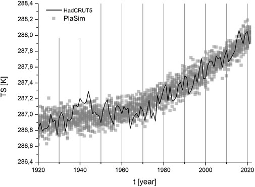
FIGURE 1. The annual global mean surface temperature TS of all the 20 members of PlaSim in the period 1920–2020 (uniform grey shading). The Met Office Hadley Centre’s observation dataset HadCRUT5 (Morice et al., 2021) is superimposed in black in the full time window.

2.2 Model convergence

It is worth noting that a climate model can only be credible if it is converged to the snapshot attractor of the climate (Deser, 2020; Herein et al., 2023). Previous studies show that the convergence time is approximately 40 years in PlaSim (Drótos et al., 2017; Drótos and Bódai, 2022), and similar values are found for more complex climate models, too (Drótos and Bódai, 2022). To ensure that we study only the converged climate data we drop the first 70 years of our simulation and consider data starting from 1920. The applied LSG ocean model is a carefully “spun up” ocean reaching a steady state numerically after around 10,000 years. To completely reach a steady state of the ocean and the vegetation to the initial climate “state” of pre-industrial conditions in 1850 [CO₂ level of 286 ppm (Lamarque et al., 2010; Taylor et al., 2012)], we integrate a single climate trajectory, which is approximately 2,000 years long. We use here the default resolution (3.5° × 3.5°) in 22 non-equidistant vertical layers with a realistic present-day bathymetry, the typical depth is 5,500 m. We emphasize, that the quoted convergence time characterizes the upper ocean and the atmosphere, while the deep ocean has a much longer characteristic time scale (hundreds of years). Since, however, we do not perturb the ocean, we can assume that its dynamics is slow enough to not affect our investigation.

3 Plume diagrams

The dynamics of the climate system is chaotic-like, possessing a high-dimensional attractor. Since we are examining a changing climate, the concept appropriate in this context is that of snapshot attractors (Romeiras et al., 1990; Ghil et al., 2008). Such an attractor represents the plethora of all permitted states at any instant of time, and ensemble simulations provide a good numerical approximation of it. When one of the parameters of the system is explicitly time-dependent (the equivalent of a changing climate), not even the long-term behavior of different single trajectories leads to the same outcome, meaning that this method does not yield representative results. An ensemble approach, however, proves to be useful in determining the snapshot attractor, a set whose shape (and probability distribution) is changing in time in a non-periodic manner (Serquina et al., 2008; Ku et al., 2015; Jánosi et al., 2021). It then follows, that in dissipative systems with explicit time-dependence, like the changing climate, the ensemble method is superior to the single-trajectory one (Tél et al., 2020). In parallel with other ideas, the ensemble approach led to the application of an increasing number of ensemble climate simulations [see, e.g., (Collins, 2007; Kay et al., 2015; Danabasoglu et al., 2020; Maher et al., 2021)]. In fact, the gray band of Figure 1 is the projection of the high-dimensional snapshot attractor on the single variable of the global mean surface temperature TS, obtained from a 20-member ensemble. Based on the above arguments, we use ensembles to follow the evolution of the detailed internal dynamics. To do this, we need a small ensemble, that is, all trajectories in this ensemble have to be initially very close to each other. In regular, non-chaotic dynamics members of such an ensemble would remain close to one another throughout the whole motion. However, one of the defining characteristics of chaos is that even small changes in the initial conditions lead to significant separation of the trajectories. This is called the sensitivity to initial conditions, or unpredictability (Ott, 1993; Tél and Gruiz, 2006). In the popular literature, this phenomenon is referred to as the butterfly effect (Gleick, 1987). Because of this, one finds that close members of the initially small ensemble quickly deviate from each other. A graphical representation of this process is provided by so-called plume diagrams. On a plume diagram, one plots one of the relevant phase space variables for all of the members of the small ensemble as a function of time, so that the fast separation in that variable can be observed.

In our study, we consider as phase space variables the global mean surface temperature (TS) and the global mean surface pressure (PS). Although the latter is a somewhat rarely used quantity in climate science, observations show a remarkable increasing trend in the surface pressure (Gillett et al., 2003; Gillett and Stott, 2009; Gillett et al., 2013) on the order of hPa-s over half a century. The changes in the pressure field could be associated with the enhanced evapotranspiration due to the warming climate. In PlaSim, we found that the trend for PS between 1950 and 2010 for the winters are compatible with the observations. We note that the emphasis of our research is not on the global surface pressure (PS), rather on its ensemble extreme behavior.

In Figure 2, we show plume diagrams with a small ensemble containing 20 members initiated in the year 1960, for TS and PS. Here, since convergence of the original ensemble has already taken place, we single out the member being initially closest to the ensemble average, and launch 20 additional trajectories around it, with random initial pressure differences on the order of Δp = 10^–8 hPa (by means of the KICK routine). After a short time (approx. 1 day) these lead to initial differences in the other variables, too. In particular, the initial temperature differences turn out to be on the order of ΔT = 10^–5 K.

FIGURE 2

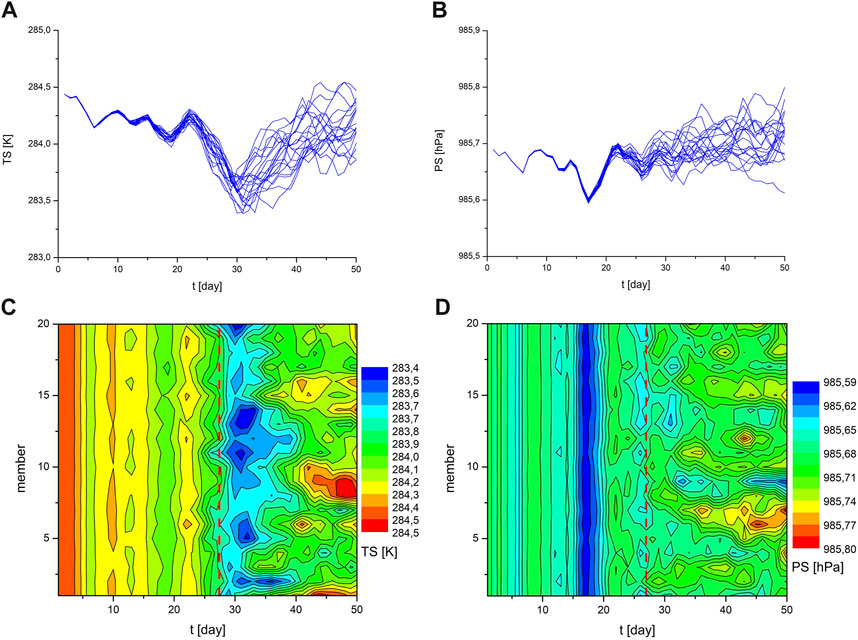
FIGURE 2. Plume diagrams showing the spread of variables (A) TS and (B) PS starting on the 1st of January 1960, over 50 days. These ensembles were created using the member of the original ensemble that was closest to the ensemble average, and scattering 20 trajectories around it with (A) order ΔT = 10⁻⁵ K temperature differences and (B) order Δp = 10⁻⁸ hPa pressure differences. We also show the time evolution of the ensemble members next to each other in panels (C,D), where the temperature and pressure values are represented as colormaps.

In panels (c) and (d), we show a novel type of representation, plotting the ensemble members next to each other (vertical axis) as a function of time, with the temperature and pressure values shown as a colormap. Since we only have 20 sub-ensemble members, the image would naturally appear quite coarse, thus for illustrative purposes we show a smoothed-out contourplot version. The labelling of the trajectories on the vertical axis does not correspond to any specific order among them, since the purpose of the image is only to show the differences between these trajectories as early as possible. The range of colors is chosen so that red and blue correspond to the maximum and minimum values within the plume diagrams. The two panels, therefore, do not start with the same color. The characteristic feature is that the panels exhibit a uniform columnar pattern first, indicating that all members carry approximately the same value. After some time, however, the pattern becomes granular with significantly different colors within the same column, corresponding to a considerable separation of the trajectories (around approximately the 27 day mark). The full pattern of each panel is thus similar to that of a flow exhibiting a transition between laminarity to turbulence about this instant. This transition is well symbolized by the dashed red vertical dividing “grid line” on panels (c) and (d), drawn at the approximate boundary between “laminarity” and “turbulence”.

It is worth noting that plume diagrams, called error growth diagrams, have recently been used in the context of baroclinic instability and its effects on extreme events in (Sheshadri et al., 2021). Their approach however, concentrates on midlatitudes, in contrast with ours which is about global averages. A more detailed comparison is given in Section 6.

4 Using sub-ensembles to obtain the extreme deviations

The traditional concept of weather and climate extreme events arose in observations as time intervals during which a measured quantity exceeded a threshold value in any direction, and their dynamics can be captured by so-called extreme climate indices (Sillmann et al., 2013b; Lee et al., 2022). These observations of course can only depict a single climate history, which is equivalent to the single trajectory/single run approach in climate simulations (Seneviratne et al., 2021). These typically refer to smaller than large-scale events which hardly turned out to be credible in climate models so far. We note however, that the potential of using climate ensembles to analyze and predict local extremes has recently begun to be explored (Bruyère et al., 2022; Franzke et al., 2023), with their trend-like behaviour studied in state-of-the-art climate models (Seneviratne et al., 2021). Being interested in global quantities, however, the concept of extremes we are after will significantly differ from those widely used in meteorology and climate science.

By accepting that the ensemble view is in general superior to the traditional one in modeling and laboratory experiments, new quantities are needed. One might consider the variance of the full ensemble, e.g., in relation to TS, the approximate width of the grey band in Figure 1. This remains, however, practically constant in time, and other climate models exhibit the same property.

We therefore propose to follow a novel approach implying a zooming in into the dynamics of the full ensemble, opening up details on a much shorter time scale. To this end as mentioned earlier, a set of small ensembles can be used, initiated close to the members of the full ensemble, generating plume diagrams. In each of them, a rapid spreading of the initially localized climate variable can be observed. If the spread of these values becomes large enough (also implying that they become considerably different from that of the original member of the full ensemble), we can call the difference between the maximum and minimum values at any instant the extreme deviation, characterizing that instant. Then, the rate at which these extreme deviations change in time can be considered as a measure of the evolution of extremes in any plume diagram. The maxima and minima are of course always given by different trajectories, since they can wander along the whole width of the plume diagram.

This “zoomed-in” characterization of extremes can result in vastly different plume diagrams. To illustrate this, we refer to Figure 3, where we show the plume diagram of sub-ensembles initiated around three different members of the full ensemble. Observe that not only the shapes are different but also the times and forms of the start of considerable spreading, implying that the extreme deviations have different time evolution in the sub-ensembles. This observation holds even if more plume diagrams are initiated. The reason for this difference is that the distribution of the data of the full ensemble, obtained on the day of the initiation of the small ensemble is extended, furthermore, it is usually not uniform either. It is natural then to take, as representative examples, three members of the full ensemble, with one being closest to the mean temperature (i.e., the one associated with the plume diagram of Figure 2, here also shown in blue), as well as the other two being closest to the standard deviation σ of the distribution, in either directions. The data of the full ensemble are represented by colored dots in Figure 3. With these three ensemble members, the plume diagrams describing the temperature and the pressure are illustrated in panels (a) and (b), respectively, of Figure 3. The colored dots are not in the same order in the two panels, since coloring is chosen to be based on temperature.

FIGURE 3

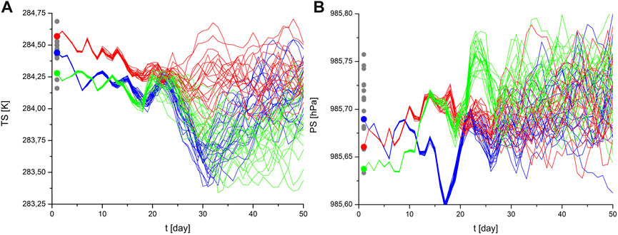
FIGURE 3. Plume diagrams initiated close to the mean and standard deviations (in either direction) of the daily temperature distribution, evaluated for the temperature (A) and the pressure (B) initiated on the first of January 1960. Red and green sub-ensembles are initiated at ± the standard deviation, σ, of TS. The initial order of the ensemble members on the vertical axis is not the same in the two panels, since both were generated using the temperature distribution, which translates to different initial conditions when evaluating the pressure. The plume diagrams shown in blue are the same as the ones depicted in Figure 2.

In order to characterize the typical growth of extremes in the full ensemble based on its distribution, some kind of averaging has to be performed. The most accurate approach would be to launch small sub-ensembles around all members of the full ensemble, generate the plume diagram for all of them, and then average over the measured extreme deviations. However, due to considerations of numerical efficiency (see next section), we will only use the three members of the full ensemble already depicted in Figure 3, to represent all the other plume diagrams. These plume diagrams, and the observed extreme deviations on them are then assigned a weight and are averaged, in order to follow the typical evolution of extremes in the full ensemble. The details of this process are discussed in the next section.

5 The time-dependence of averaged extreme deviations

Our goal is to quantitatively characterize the increase of the spread of extremes based on the plume diagrams of Figure 3. To this end we recall (Ott, 1993; Tél and Gruiz, 2006) that the spread of the difference between initially nearby trajectories is characterized by the so-called Lyapunov exponent. This is evaluated by considering trajectory pairs of initial phase space distance Δr₀ and following the time evolution Δr(t) of this distance. Taking several such trajectory pairs, and performing the average over this ensemble, the (largest) Lyapunov exponent is the initial slope λ of the quantity

$\mathrm{\Lambda }\left(t\right)=⟨\ln \frac{\mathrm{\Delta }r\left(t\right)}{\mathrm{\Delta }{r}_0}⟩,(1)$

where the bracket denotes average taken over an ensemble. The logarithm is taken since the differences are expected to grow in chaos, on average, exponentially in time. It is worth emphasizing that the Lyapunov exponent, by this definition, only describes the initial behavior of the trajectories. We note that the investigation of the Lyapunov exponent of climate models is of current interest, and not only the largest exponent but even the spectrum of such exponents can be determined, as e.g., in (De Cruz et al., 2018).

Here, instead of phase space distances, we are interested in differences of extremes. This means, that we are not interested in determining the Lyapunov exponent in the climate model (since it is not about extremes), rather, we use (Eq. 1) as a guide when examining the magnitude of extreme deviations in time. Considering an arbitrary variable of the climate model A in a plume diagram, one can determine its maximum and minimum value, A_max(t) and A_min(t), respectively, at any instant of time. As an analog of Δr(t), we consider the difference A_max(t) − A_min(t) between extremal values. For normalization, we take the full spread ΔA₀ of the full ensemble at the start of the plume diagram. We thus concentrate on the quantity

$\mathrm{\Gamma }\left(t\right)=⟨{\left[\ln \frac{A_{\mathit{max}}\left(t\right)-A_{\mathit{min}}\left(t\right)}{\mathrm{\Delta }{A}_0}\right]}_N⟩,(2)$

where the inner bracket indicates that the extrema are taken over the small ensemble of size N of a single plume diagram and the outer bracket denotes the average over the full ensemble of the climate simulation. We propose to call Γ(t) the Double-Ensemble Extreme Deviation (DEED). Its initial slope γ characterizes the increase of the differences between the extremes of quantity A, and is going to be called the growth rate of extremes.

Distinguishing small ensembles and plume diagrams by index j within the full ensemble of size M, quantity (Eq. 2) can be written as

$\mathrm{\Gamma }\left(t\right)=\frac{1}{M}\sum _j{\left[\ln \frac{A_{\mathit{max}j}\left(t\right)-A_{\mathit{min}j}\left(t\right)}{\mathrm{\Delta }{A}_0}\right]}_N=\frac{1}{M}\sum _j{\mathrm{\Gamma }}_j(3)$

The uniform summation over the full ensemble implies a natural weighting, since more members of the full ensemble fall close to the ensemble mean than to, say, the standard deviations σ₊ or σ₋ above and below the mean. The evaluation of this sum requires the evaluation of altogether N ⋅ M ensemble members.

Following the original, full climate ensemble of size M = 20 according to (Eq. 3) would require 20 sub-ensembles, technically resulting in a 400-element ensemble with daily time resolution. However, for numerical efficiency and based on our previous experiences (Herein et al., 2023), we now follow a simplified approach with three representative 20-member sub-ensembles, corresponding to a 60-member ensemble. It is known to be usually sufficient to examine ensembles with a relatively low number of members to gain a proper characterization of internal variability for global quantities, at least [see (Milinski et al., 2020) concerning variable TS]. It has been shown in (Milinski et al., 2020; Pierini, 2020) that one can have acceptable statistics starting from a few tens of members, which is indeed the case for us.

Out of all possible small ensembles, we take the three representative members, the ones shown in Figure 3, one initiated around the mean and two others at about a distance σ₊ and σ₋ away. The corresponding Γ_j-s will be denoted by Γ₀, Γ₊, and Γ₋, respectively. The averaging over the full ensemble is replaced by associating weights w₀ and w₊, w₋ < w₀ (w₀ + w₊ + w₋ = 1) to these plume diagrams. The sum is then replaced by

$\mathrm{\Gamma }\left(t\right)\approx w_0{\mathrm{\Gamma }}_0\left(t\right)+w_{+}{\mathrm{\Gamma }}_{+}\left(t\right)+w_{-}{\mathrm{\Gamma }}_{-}\left(t\right).(4)$

The choice of the weights is somewhat subjective. The daily temperature distribution of the sub-ensembles of the initial 50 days reliably (p-value between 0.3–0.9, with the standard alpha significance level of 0.05) passes the Shapiro-Wilk test (Shapiro and Wilk, 1965), so we can say that the temperature distribution is not in contradiction with a standard normal distribution. We then choose w₀ as the maximum and w₊ = w₋ as the variance value of the standard distribution. These are w₀ = 0.45, w₊ = w₋ = 0.275.

In chaos theory the typical time-dependence of the phase space distance is estimated as Δr(t) ∼ e^λt. In analogy with this, we also expect to see an exponential growth on average of the extreme deviations approximated as

$A_{\mathit{max}}\left(t\right)-A_{\mathit{min}}\left(t\right)\sim e^{\gamma t},(5)$

where γ is the growth rate of extremes. In Figure 4 we show the time evolution of Γ, that is the DEED quantity in the first 50 days of 1960. We can clearly observe, in analogy with the Lyapunov exponent, an initial exponential growth. The slope of the fitted red linear curve is then the above-mentioned growth rate of extremes, γ. The fit is taken over the linear range of the graphs, which is a standard practice in chaos theory. Its value for the temperature (panel a) is γ_TS = 0.163 ± 0.006 (1/day), while for the pressure (panel b) γ_PS = 0.245 ± 0.005 (1/day).

FIGURE 4

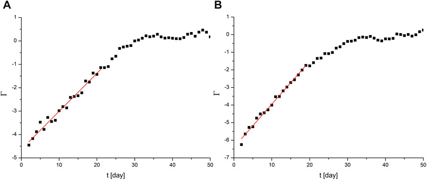
FIGURE 4. The time evolution of DEED for temperature TS (A) and pressure PS (B). The red curves indicate the linear fit to the initial, exponential phase, from which the slopes γ_TS = 0.163 (1/day) and γ_PS = 0.245 (1/day) are obtained.

We can also observe that the DEED value quickly goes into saturation (compared to the time scale of the climate model), the time scale of measuring the growth rate of extremes is thus quite small, around 20 days, which is nowhere near the about 40 years required for the convergence to the climate attractor. This means that we cannot obtain representative information about the changing climate by measuring γ in only one year. We can, however, precisely because of the short time scale, associate γ to the year it was measured in. It gives the initial slope of the DEED curve, that is, the growth rate of the extremes at the beginning of that year. It naturally follows then, that we are able to characterize the changing climate by measuring γ in different years and follow its value as time goes on.

We could now plot γ in each investigated year, but instead we turn to a more natural value, in analogy with chaos theory, where the reciprocal of the λ Lyapunov exponent is understood as the so-called Lyapunov time, the time until trajectories of a plume diagram remain close to each other. Since the γ growth rate of extremes is also derived based on plume diagrams, we can now make an analogy with the Lyapunov time and associate a characteristic time with the emergence of extremes as the quantity 1/γ. This will describe the time after which large differences (i.e., the extreme deviations) can occur in the plume diagrams.

We measured this extreme emergence time (EET) for every 10 years between 1920 and 2020, the results of which can be seen in Figure 5, with the errorbars indicating the fitting errors of γ in each case. Since 1958 is the start of precise CO₂ measurements (Keeling et al., 2001) and CO₂ growth shows a significant positive trend since then, our expectation is that any pronounced effects might appear from here onwards. For the pressure (panel b) before around 1960 the EET values are close to constant, however, after this point they exhibit a decreasing linear trend, supporting our hypothesis in this case. Then we can say that we can observe the effect of climate change in the EET of this variable, suggesting that the emergence of extreme deviations in the global surface pressure might occur earlier in a climate change as time goes on.

FIGURE 5

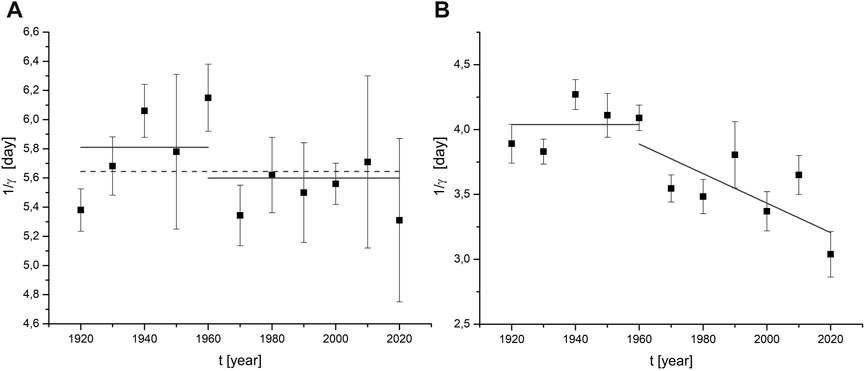
FIGURE 5. Reciprocals of the γ slopes, the EETs (day) for discrete years with estimated errors of linear fits for temperature TS (A) and pressure PS (B). The dashed line in panel (A) shows the time average over the whole period, while the solid lines indicate the averages before and after 1960. In panel (B), the solid line represents the average before 1960, and after 1960 a linear fit was applied to the data, resulting in a slope of about 1 day/100 years, also symbolized by a solid line.

The results for the temperature (panel a) are different. Here, the pre-1960 time period can also be characterized by a constant. (One might see an increasing trend, but due to the rather large errorbars, we do not think that any higher-than-zero order trends can be convincingly identified.) However, in this case climate change seemingly does not induce any trend whatsoever, only a small jump in the average can be observed. Alternatively, one can also easily come to the conclusion that the EET is constant throughout the whole investigated time interval, which is denoted by the dashed line.

It might be surprising to see that the typical characteristic times in panels (a) and (b) differ by about 1 day. However, there are no restrictions set on the emergence time of the extremes in different variables, here in temperature and pressure, needing be the same. It is also worth noting that the naked eye does not recognize that a strong spreading of the plume diagrams is starting at different times, e.g., in Figure 2. Initially the values are so close that the eye does not see other than a single curve. The orders of magnitude of the initial differences can be extracted from the logarithmic fits of Figure 4, where we see that they are much smaller for the pressure. However, at the end of the initial deviation process (red line) the orders of magnitude are about the same, meaning that the slope for the pressure is larger, as the γ values in the caption of Figure 4 indicate.

6 Outlook

For illustrative purposes in Figure 6 we show the considerable regional differences between two ensemble members exhibiting maximum and minimum behavior in a global quantity on a given day, and compare them in different years. We show the maximum pressure difference within one chosen plume diagram on a day where the differences are considerable (on February 11) in the years 1950 (panel a) and in 2010 (panel b) in PlaSim.

FIGURE 6

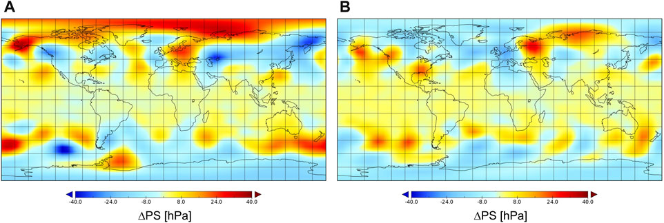
FIGURE 6. The map of the instantaneous pressure difference between daily maxima and minima (ΔPS) (A) on 11 February 1950 and (B) on 11 February 2010 in Plasim.

Although one sees remarkable maxima and minima in the pressure difference field at different geographical locations, we do not consider these to be worth discussing since the widely accepted ensemble view followed in our approach implies that none of the individual simulations are representative. Nevertheless, these images might provide an impression of the local inhomogeneities of the possible extremes of the surface pressure.

It is also worth mentioning here a similar issue, the growth rate of perturbations in baroclinic instability. The growth rate σ of the most unstable wavenumber is known to be (Gill, 1982; Pedlosky, 1987):

$\sigma =c\frac{f}{N}\frac{d{u}_0}{dz}(6)$

where f and N represent the Coriolis parameter and the Brunt-Väisälä frequency, respectively, while du₀/dz is the vertical shear of the thermal wind. Coefficient c depends on the model, but is always of order unity. In the so-called Eady model, it takes the value c = 0.31, and the reciprocal of σ, the e-folding time of perturbations is about 2 days (Gill, 1982). In spite of the similar orders of magnitude of 1/γ and 1/σ, the physics is dramatically different. In baroclinic instability, the growth rate describes how the velocity deviation from the unperturbed flow initially increases:

$u\left(t\right)-u_0\sim e^{\sigma t},(7)$

and it sets the time over which small amplitude waves develop from a horizontally homogeneous flow. These waves are, however, not yet broken and are thus not turbulent. The quantity σ is related to the very first phase of the emergence of an instability in a flow in which neighboring trajectories do not yet diverge, and are not yet chaotic. In contrast, the plume diagrams characterize the chaotic-like behavior of the atmospheric/climatic dynamics governed by turbulence (which is indeed the ultimate state of baroclinic instability). Another reason to call the two approaches dramatically different is that the growth rate is instantaneous and local (most dramatically due to the presence of f), while γ is about a history (over weeks) and refers to globally averaged quantities.

There is considerable literature on the Eady growth rate and its temporal change since the latter is considered to indicate changes in the baroclinicity, the mechanism by which cyclones, fronts, and other weather systems are generated [see, e.g., (Lehmann et al., 2014; Sheshadri et al., 2021; Simmonds and Li, 2021)]. The resuls are season and location, even hemisphere, dependent. In (Lehmann et al., 2014) a relation is found between changes in the storm tracks and changes in the maximum Eady growth rate at mid-latitudes. The authors of (Sheshadri et al., 2021) find relation between what they call the time to error saturation, the analog of the time needed to reach an approximate plateau in our plume diagrams, and the Eady growth rate. Their conclusion is that midlatitude weather may be less predictable in warmer climates. The study of (Simmonds and Li, 2021) includes also the polar regions, and finds that arctic sea ice loss can be associated with an increase in Eady growth rate. This paper also provides maps of the local Eady growth rate and its trend in all seasons and for both hemispheres. Their Figure 6 exhibits very strong variability in all panels indicating trends of the same magnitude with both signs. A properly carried out annual averaging of these trends over the Globe could provide a quantity that would be similar in spirit to our extreme emergence time (EET). The Eady growth rate related studies do provide useful insight into extremes, providing characteristic values similar to ours concerning orders of magnitudes, however our approach appears to be the only one consistent with single initial condition large ensemble simulations providing global values.

7 Conclusion

According to the traditional picture, extreme events are defined on the basis of observations and single-run simulations, and cannot be easily interpreted in the world of ensembles. Therefore, we propose here a new ensemble approach to follow the global dynamics of extremes under climate change. The idea is to create an original, full ensemble and zoom into it with the initialization of small sub-ensembles at discrete, chosen time instants, to detect the typical behavior of the extremes. Small ensembles are “small” in the sense that their members are very close to each other in the beginning. Plume diagrams initiated on the same day of a year are generated from these sub-ensembles. The trajectories within a plume diagram strongly deviate on the time scale of a few weeks. Extreme deviations then are defined as the instantaneous difference between the maximum and minimum values of a given quantity in the plume diagram. We follow this instantaneous difference in time and call the separation rate as the growth rate of extremes. By averaging over all sub-ensembles, we get the typical growth rate and with its reciprocal we are able to measure the characteristic time of the emergence of extremes. Our growth rate of extremes might be seen as similar to the Eady growth rate studied in the literature, but the former reflects the chaotic behavior of the already converged climate attractor, while the numerical value of the latter characterizes the initial, “laminar” state before approaching the attractor.

To illustrate the above-presented approach we have used the climate model PlaSim to run a 20-member ensemble simulation with historical and observed CO₂ forcing, providing a full climate ensemble. To detect the possible behavior of extremes in the model, we generated the small sub-ensembles around three members of the full ensemble and calculated the characteristic time of the emergence of extremes. This is found to be on the order of a few days, however, it can be slightly different for different variables. We showed that the characteristic time for the global mean surface temperature remains practically constant during climate change. At the same time, this does not hold for the global mean surface pressure since a pronounced decreasing trend is found, with a slope of 1 day/century.

We note that, aside from plume diagrams, other methods originating in chaotic dynamics could also be utilized to characterize global climate variables. For example, the recently developed method of EAPD (ensemble-averaged pairwise distance) (Jánosi and Tél, 2022), which monitors the phase space distance between trajectories in an ensemble, seems particularly well suited for problems requiring an ensemble approach. The application of such methods could be the subject of future papers.

As a final conclusion, we say that our approach can be integrated into any other climate model being credible in global quantities, and it can be especially useful to test in state-of-the-art climate models (e.g., SMILEs), to properly unfold the dynamics of global extremes. With the improvement of these models, there is a potential benefit in following the geographical evolution of extremes as well.

Data availability statement

The raw data supporting the conclusion of this article will be made available by the authors, without undue reservation.

Author contributions

MH: Conceptualization, Data curation, Investigation, Visualization, Writing–original draft, Formal Analysis, Methodology, Software, Writing–review and editing. DJ: Conceptualization, Data curation, Formal Analysis, Investigation, Methodology, Validation, Writing–original draft, Writing–review and editing. TT: Conceptualization, Methodology, Supervision, Writing–original draft, Writing–review and editing.

Funding

The author(s) declare financial support was received for the research, authorship, and/or publication of this article. This work was supported by the Hungarian National Research, Development and Innovation Office (NKFIH) under Grants K125171 (all authors), FK135115 (MH), and K128584 (DJ). MH was supported by the János Bolyai Research Scholarship of the Hungarian Academy of Sciences. DJ benefited from the New National Excellence Program (ÚNKP) scholarship of the NKFIH office, under grant no. ÚNKP-22-3-I-ELTE-199.

Acknowledgments

Fruitful discussions with Tímea Haszpra, Zoltán Trócsányi, and Miklós Vincze are acknowledged. Thanks are due to András Herein and Róbert Mészáros for providing useful suggestions.

Conflict of interest

The authors declare that the research was conducted in the absence of any commercial or financial relationships that could be construed as a potential conflict of interest.

Publisher’s note

All claims expressed in this article are solely those of the authors and do not necessarily represent those of their affiliated organizations, or those of the publisher, the editors and the reviewers. Any product that may be evaluated in this article, or claim that may be made by its manufacturer, is not guaranteed or endorsed by the publisher.

References

Ansmann, G., Karnatak, R., Lehnertz, K., and Feudel, U. (2013). Extreme events in excitable systems and mechanisms of their generation. Phys. Rev. E Stat. Nonlin Soft Matter Phys. 88 (5), 052911. doi:10.1103/PhysRevE.88.052911

PubMed Abstract | CrossRef Full Text | Google Scholar

Bódai, T. (2015). Predictability of threshold exceedances in dynamical systems. Phys. D. 313, 37–50. doi:10.1016/j.physd.2015.08.007

CrossRef Full Text | Google Scholar

Bruyère, C. L., Buckley, B., Jaye, A. B., Done, J. M., and Leplastrier, M. (2022). Joanna Aldridge, Peter Chan, Erin Towler, Ming Ge, Using large climate model ensembles to assess historical and future tropical cyclone activity along the Australian east coast. Weather Clim. Extrem. 38, 00507. doi:10.1016/j.wace.2022.100507

CrossRef Full Text | Google Scholar

Collins, M. (2007). Ensembles and probabilities: a new era in the prediction of climate change. Philos. Trans. R. Soc. A 365, 1957–1970. doi:10.1098/rsta.2007.2068

PubMed Abstract | CrossRef Full Text | Google Scholar

Danabasoglu, G., Lamarque, J.-F., Bacmeister, J., Bailey, D. A., DuVivier, A. K., Edwards, J., et al. (2020). The community earth system model version 2 (CESM2). J. Adv. Model. Earth Syst. 12, e2019MS001916. doi:10.1029/2019ms001916

CrossRef Full Text | Google Scholar

De Cruz, L., Schubert, S., Demaeyer, J., Lucarini, V., and Vannitsem, S. (2018). Exploring the Lyapunov instability properties of high-dimensional atmospheric and climate models. Nonlin. Proc. Geophys. 25, 387–412. doi:10.5194/npg-25-387-2018

CrossRef Full Text | Google Scholar

Deser, C. (2020). Certain uncertainty: the role of internal climate variability in projections of regional climate change and risk management. Earth’s Future 8, e2020EF001854. doi:10.1029/2020ef001854

CrossRef Full Text | Google Scholar

Deser, C., Phillips, A. S., Simpson, I. R., Rosenbloom, N., Coleman, D., Lehner, F., et al. (2020). Isolating the evolving contributions of anthropogenic aerosols and greenhouse gases: a New CESM1 large ensemble community resource. J. Clim. 33 (18), 7835–7858. doi:10.1175/jcli-d-20-0123.1

CrossRef Full Text | Google Scholar

Drótos, G., and Bódai, T. (2022). On defining climate by means of an ensemble. Authorea, 1–35. doi:10.1002/essoar.10510833.3

CrossRef Full Text | Google Scholar

Drótos, G., Bódai, T., and Tél, T. (2017). On the importance of the convergence to climate attractors. Eur. Phys. J. Spec. Top. 226, 2031–2038. doi:10.1140/epjst/e2017-70045-7

CrossRef Full Text | Google Scholar

Folis, W. W., and Hide, R. (1965). Thermal convection in a rotating annulus of liquid: effect of viscosity on the transition between axisymmetric and non-axisymmetric flow regimes. J. Atmos. Sci. 22, 541–558. doi:10.1175/1520-0469(1965)022<0541:tciara>2.0.co;2

CrossRef Full Text | Google Scholar

Fraedrich, K., Jansen, H., Kirk, E., Luksch, U., and Lunkeit, F. (2005). The planet simulator: towards a user friendly model. Meteorol. Z. 14 (3), 299–304. doi:10.1127/0941-2948/2005/0043

CrossRef Full Text | Google Scholar

Francis, J. A., and Stephen, J. (2015) Evidence for a wavier jet stream in response to rapid Arctic warming. Environ. Res. Lett. 10, 014005. doi:10.1088/1748-9326/10/1/014005

CrossRef Full Text | Google Scholar

Franzke, C. L. E. (2022). Changing temporal volatility of precipitation extremes due to global warming. Int. J. Climatol. 42 (16), 8971–8983. doi:10.1002/joc.7789

CrossRef Full Text | Google Scholar

Franzke, C. L. E., Lee, J. Y., O’Kane, T., Merryfield, W., and Zhang, X. (2023). Extreme weather and climate events: dynamics, predictability and ensemble simulations. Asia-Pac J. Atmos. Sci. 59, 1–2. doi:10.1007/s13143-023-00317-5

CrossRef Full Text | Google Scholar

Fultz, D., and Long, R. R. (1951). Two-dimensional flow around a circular barrier in a rotating spherical shell. Tellus 3 (2), 61–68. doi:10.3402/tellusa.v3i2.8623

CrossRef Full Text | Google Scholar

Ghil, M., Chekroun, M. D., and Simonnet, E. (2008). Climate dynamics and fluid mechanics: natural variability and related uncertainties. Phys. D. 237, 2111–2126. doi:10.1016/j.physd.2008.03.036

CrossRef Full Text | Google Scholar

Ghil, M., and Lucarini, V. (2020). The physics of climate variability and climate change. Rev. Mod. Phys. 92, 035002. doi:10.1103/revmodphys.92.035002

CrossRef Full Text | Google Scholar

Gill, A. E. (1982). Atmosphere-Ocean dynamics. Academic Press.

Google Scholar

Gillett, N., Zwiers, F., Weaver, A., and Stott, P. A. (2003). Detection of human influence on sea-level pressure. Nature 422, 292–294. doi:10.1038/nature01487

PubMed Abstract | CrossRef Full Text | Google Scholar

Gillett, N. P., Fyfe, J. C., and Parker, D. E. (2013). Attribution of observed sea level pressure trends to greenhouse gas, aerosol, and ozone changes. Geophys. Res. Lett. 40, 2302–2306. doi:10.1002/grl.50500

CrossRef Full Text | Google Scholar

Gillett, N. P., and Stott, P. A. (2009). Attribution of anthropogenic influence on seasonal sea level pressure. Geophys. Res. Lett. 36, L23709. doi:10.1029/2009GL041269

CrossRef Full Text | Google Scholar

Gleick, J. (1987). Chaos: making a new science. New York: Viking Press.

Google Scholar

Harlander, U., Borcia, I. D., Vincze, M., and Rodda, C. (2022). Probability distribution of extreme events in a baroclinic wave laboratory experiment. Fluids 7, 274. doi:10.3390/fluids7080274

CrossRef Full Text | Google Scholar

Herein, M., Drótos, G., Haszpra, T., Márfy, J., and Tél, T. (2017). The theory of parallel climate realizations as a new framework for teleconnection analysis. Sci. Rep. 7, 44529. doi:10.1038/srep44529

PubMed Abstract | CrossRef Full Text | Google Scholar

Herein, M., Tél, T., and Haszpra, T. (2023). Where are the coexisting parallel climates? Large ensemble climate projections from the point of view of chaos theory. Chaos 33, 031104. doi:10.1063/5.0136719

PubMed Abstract | CrossRef Full Text | Google Scholar

S. C. Herring, M. P. Hoerling, T. C. Peterson, P. A. Stott, and C. Schär (Editors) (2015). Attribution of extreme weather events in the context of climate change (National Academies Press).

Google Scholar

Inness, P., and Dorling, S. (2013). Advancing weather and climate science. Wiley-Blackwell, pp231. 9780470711590.Operational weather forecasting.

Google Scholar

Jánosi, D., Károlyi, G., and Tél, T. (2021). Climate change in mechanical systems: the snapshot view of parallel dynamical evolutions. Nonlinear Dyn. 106, 2781–2805. doi:10.1007/s11071-021-06929-8

CrossRef Full Text | Google Scholar

Jánosi, D., and Tél, T. (2022). Characterizing chaos in systems subjected to parameter drift. Phys. Rev. E 105, L062202. doi:10.1103/physreve.105.l062202

PubMed Abstract | CrossRef Full Text | Google Scholar

Kay, J. E., Deser, C., Phillips, A., Mai, A., Hannay, C., Strand, G., et al. (2015). The community earth system model (CESM) large ensemble project: a community resource for studying climate change in the presence of internal climate variability. Bull. Am. Meteorol. Soc. 96, 1333–1349. doi:10.1175/bams-d-13-00255.1

CrossRef Full Text | Google Scholar

Keeling, C. D., Piper, S. C., Bacastow, R. B., Wahlen, M., Whorf, T. P., Heimann, M., et al. (2001). Exchanges of atmospheric CO2 and CO2 with the terrestrial biosphere and oceans from 1978 to 2000. I. Global aspects, SIO Reference Series, No. 01-06. San Diego: Scripps Institution of Oceanography.

Google Scholar

Kleidon, A. (2006). The climate sensitivity to human appropriation of vegetation productivity and its thermodynamic characterization. Glob. Planet Change 54, 109–127. doi:10.1016/j.gloplacha.2006.01.016

CrossRef Full Text | Google Scholar

Knutson, T., McBride, J., Chan, J., Emanuel, K., Holland, G., Landsea, C., et al. (2010). Tropical cyclones and climate change. Nature Geosci. 3, 157–163. doi:10.1038/ngeo779

CrossRef Full Text | Google Scholar

Ku, W. L., Girvan, M., and Ott, E. (2015). Dynamical transitions in large systems of mean field-coupled Landau-Stuart oscillators: extensive chaos and cluster states. Chaos 25, 123122. doi:10.1063/1.4938534

PubMed Abstract | CrossRef Full Text | Google Scholar

Lamarque, J.-F., Bond, T. C., Eyring, V., Granier, C., Heil, A., Klimont, Z., et al. (2010). Historical (1850–2000) gridded anthropogenic and biomass burning emissions of reactive gases and aerosols: methodology and application. Atmos. Chem. Phys. 10, 7017–7039. doi:10.5194/acp-10-7017-2010

CrossRef Full Text | Google Scholar

Lee, Y. K., Kim, H. S., Kim, J. E., Choi, Y. S., and Yoo, C. (2022). Markov chain analysis of rainfall over east asia: unusual frequency, persistence, and entropy in the summer 2020. J. Atmos. Sci. 58, 281–291. doi:10.1007/s13143-021-00255-0

CrossRef Full Text | Google Scholar

Lehmann, J., Coumou, D., Frieler, K., Eliseev, A. V., and Levermann, A. (2014). Future changes in extratropical storm tracks and baroclinicity under climate change. Environ. Res. Lett. 9 (8), 084002. doi:10.1088/1748-9326/9/8/084002

CrossRef Full Text | Google Scholar

Li, X., Ding, R., and Li, J. (2022). A new technique to quantify the local predictability of extreme events: the backward nonlinear local Lyapunov exponent method. Front. Environ. Sci. 10, 825233. doi:10.3389/fenvs.2022.825233

CrossRef Full Text | Google Scholar

Lucarini, V., Faranda, D., Wouters, J., and Kuna, T. (2014). Towards a general theory of extremes for observables of chaotic dynamical systems. J. Stat. Phys. 154, 723–750. doi:10.1007/s10955-013-0914-6

PubMed Abstract | CrossRef Full Text | Google Scholar

Lucarini, V., Fraedrich, K., and Lunkeit, F. (2010). Thermodynamic analysis of snowball Earth hysteresis experiment: efficiency, entropy production and irreversibility. Q.J.R. Meteorol. Soc. 136, 2–11. doi:10.1002/qj.543

CrossRef Full Text | Google Scholar

Lunkeit, F., Fraedrich, K., Jansen, H., Kirk, E., Kleidon, A., and Luksch, U., (2011). Planet Simulator reference manual, available at https://www.mi.uni168hamburg.de/en/arbeitsgruppen/theoretische-meteorologie/modelle/plasim.html.

Google Scholar

Maher, N., Milinski, S., and Ludwig, R. (2021). Large ensemble climate model simulations: introduction, overview, and future prospects for utilising multiple types of large ensemble. Earth Syst. Dyn. 12, 401–418. doi:10.5194/esd-12-401-2021

CrossRef Full Text | Google Scholar

Maier-Reimer, E., and Mikolajewicz, U. (1991). The Hamburg large scale Geostrophic Ocean 170 general circulation model (cycle 1), 2. Technical Report/Deutsches Klimarechenzentrum.

Google Scholar

Maier-Reimer, E., Mikolajewicz, U., and Hasselmann, K. (1993). Mean circulation of the Hamburg LSG OGCM and its sensitivity to the thermohaline surface forcing. J. Phys. Oceanogr. 23, 731–757. doi:10.1175/1520-0485(1993)023<0731:mcothl>2.0.co;2

CrossRef Full Text | Google Scholar

Milinski, S., Maher, N., and Olonscheck, D. (2020). How large does a large ensemble need to be? Earth Syst. Dyn. 11 (4), 885–901. doi:10.5194/esd-11-885-2020

CrossRef Full Text | Google Scholar

Mishra, A., Leo Kingston, S., Hens, C., Kapitaniak, T., Feudel, U., and Dana, S. K. (2020). Routes to extreme events in dynamical systems: dynamical and statistical characteristics. Chaos 30, 063114. doi:10.1063/1.5144143

PubMed Abstract | CrossRef Full Text | Google Scholar

Morice, C. P., Kennedy, J. J., Rayner, N. A., Winn, J. P., Hogan, E., Killick, R. E., et al. (2021). An updated assessment of near-surface temperature change from 1850: the HadCRUT5 data set. J. Geophys. Res. Atmos. 126, e2019JD032361. doi:10.1029/2019jd032361

CrossRef Full Text | Google Scholar

Ott, E. (1993). Chaos in dynamical systems. Cambridge: Cambridge U. Press.

Google Scholar

Pedlosky, J. (1987). Geophysical fluid dynamics. Springer.

Google Scholar

Pierini, S. (2020). Statistical significance of small ensembles of simulations and detection of the internal climate variability: an excitable ocean system case study. J. Stat. Phys. 179, 1475–1495. doi:10.1007/s10955-019-02409-x

CrossRef Full Text | Google Scholar

Pierini, S., and Ghil, M. (2021). Tipping points induced by parameter drift in an excitable ocean model. Sci. Rep. 11, 11126. doi:10.1038/s41598-021-90138-1

PubMed Abstract | CrossRef Full Text | Google Scholar

Rodda, C., Harlander, U., and Vincze, M. (2022). Jet stream variability in a polar warming scenario – a laboratory perspective. Weather Clim. Dynam. 3, 937–950. doi:10.5194/wcd-3-937-2022

CrossRef Full Text | Google Scholar

Romeiras, F. J., Grebogi, C., and Ott, E. (1990). Multifractal properties of snapshot attractors of random maps. Phys. Rev. A 41, 784–799. doi:10.1103/physreva.41.784

PubMed Abstract | CrossRef Full Text | Google Scholar

Seneviratne, S. I., Zhang, X., Adnan, M., Badi, W., Dereczynski, C., Di Luca, A., et al. (2021). “Weather and climate extreme events in a changing climate,” in Climate change 2021: the physical science basis. Contribution of working group I to the sixth assessment report of the intergovernmental panel on climate change [Masson-Delmotte, V. Editors P. Zhai, A. Pirani, S. L. Connors, C. Péan, S. Berger, N. Caudet al. (Cambridge, United Kingdom and New York, NY, USA: Cambridge University Press), 1513–1766. doi:10.1017/9781009157896.013

CrossRef Full Text | Google Scholar

Serquina, R., Lai, Y.-C., and Chen, Q. (2008). Characterization of nonstationary chaotic systems. Phys. Rev. E 77, 026208. doi:10.1103/physreve.77.026208

PubMed Abstract | CrossRef Full Text | Google Scholar

Shapiro, S. S., and Wilk, M. B. (1965). An analysis of variance test for normality (complete samples). Biometrika 52 (3–4), 591–611. doi:10.1093/biomet/52.3-4.591

CrossRef Full Text | Google Scholar

Shaw, T. A., Baldwin, M., Barnes, E. A., Caballero, R., Garfinkel, C. I., Hwang, Y. T., et al. (2016). Storm track processes and the opposing influences of climate change. Nat. Geosci. 9 (9), 656–664. doi:10.1038/ngeo2783

CrossRef Full Text | Google Scholar

Sheshadri, A., Borrus, M., Yoder, M., and Robinson, T. (2021). Midlatitude error growth in atmospheric GCMs: the role of eddy growth rate. Geophys. Res. Lett. 48, 23. doi:10.1029/2021gl096126

CrossRef Full Text | Google Scholar

Sillmann, J., Kharin, V. V., Zhang, X., Zwiers, F. W., and Bronaugh, D. (2013a). Climate extremes indices in the CMIP5 multimodel ensemble: Part 1. Model evaluation in the present climate. J. Clim. 26 (3), 1716–1733. doi:10.1002/jgrd.50203

CrossRef Full Text | Google Scholar

Sillmann, J., Kharin, V. V., Zwiers, F. W., Zhang, X., and Bronaugh, D. (2013b). Climate extremes indices in the CMIP5 multimodel ensemble: Part 2. Future climate projections. J. Geophys. Res. Atmos. 118, 2473–2493. doi:10.1002/jgrd.50188

CrossRef Full Text | Google Scholar

Simmonds, I., and Li, M. (2021). Trends and variability in polar sea ice, global atmospheric circulations, and baroclinicity. Ann. N.Y. Acad. Sci. 1504 (1), 167–186. doi:10.1111/nyas.14673

PubMed Abstract | CrossRef Full Text | Google Scholar

Stendel, M., Francis, J., White, R., Williams, P. D., and Woollings, T. (2021). “Chapter 15—the jet stream and climate change,” in Climate change. Editor T. M Letcher. 3rd ed. (Amsterdam, The Netherlands: Elsevier), 327–357.

CrossRef Full Text | Google Scholar

Suárez-Gutiérrez, L., Milinski, S., and Maher, N. (2021). Exploiting large ensembles for a better yet simpler climate model evaluation. Clim. Dyn. 57, 2557–2580. doi:10.1007/s00382-021-05821-w

CrossRef Full Text | Google Scholar

Sun, X., Ding, Q., Wang, S. Y. S., Topál, D., Li, Q., Castro, C., et al. (2022). Enhanced jet stream waviness induced by suppressed tropical Pacific convection during boreal summer. Nat. Commun. 13, 1288. doi:10.1038/s41467-022-28911-7

PubMed Abstract | CrossRef Full Text | Google Scholar

Taylor, K. E., Stouffer, R. J., and Meehl, G. A. (2012). An overview of CMIP5 and the experiment design. Bull. Am. Meteorol. Soc. 93, 485–498. doi:10.1175/bams-d-11-00094.1

CrossRef Full Text | Google Scholar

Tél, T., Bódai, T., Drótos, G., Haszpra, T., Herein, M., Kaszás, B., et al. (2020). The theory of parallel climate realizations, A new framework of ensemble methods in a changing climate: an overview. J. Stat. Phys. 179, 1496–1530. doi:10.1007/s10955-019-02445-7

CrossRef Full Text | Google Scholar

Tél, T., and Gruiz, M. (2006). Chaotic dynamics. Cambridge, New York.

Google Scholar

Tokarska, K. B., Stolpe, M. B., Sippel, S., Fischer, E. M., Smith, C. J., Lehner, F., et al. (2020). Past warming trend constrains future warming in CMIP6 models. Sci. Adv. 6 (12), eaaz9549. doi:10.1126/sciadv.aaz9549

PubMed Abstract | CrossRef Full Text | Google Scholar

Vincze, M., Borcia, I. D., and Harlander, U. (2017). Temperature fluctuations in a changing climate: an ensemble based experimental approach. Sci. Rep. 7, 254. doi:10.1038/s41598-017-00319-0

PubMed Abstract | CrossRef Full Text | Google Scholar

Vincze, M., Bozóki, T., Herein, M., Borcia, I. D., Harlander, U., Horicsányi, A., et al. (2021). The Drake Passage opening from an experimental fluid dynamics point of view. Sci. Rep. 11, 19951. doi:10.1038/s41598-021-99123-0

PubMed Abstract | CrossRef Full Text | Google Scholar