Topographic controls of water balance response to air temperature increase in permafrost-affected watersheds

1 Introduction

In recent decades an increase in freshwater runoff to the Arctic ocean (especially during the cold period of the year) has been observed for Eurasian (Stuefer et al., 2011; Shiklomanov et al., 2013; Tan and Gan, 2015; Déry et al., 2016; Tananaev et al., 2016) and North American (Shiklomanov and Lammers, 2011; Déry et al., 2016; Holmes et al., 2018) basins. However, recently observed trends in annual precipitation over these basins are not large enough to support this increase in runoff (Berezovskaya et al., 2004; Adam and Lettenmaier, 2008; Bring and Destouni, 2011; Bring et al., 2016; Panyushkina et al., 2021; Wang et al., 2021). On the other hand, the widespread increase in air temperature (Biskaborn et al., 2019) has been well documented. On regional and local scales, many studies (Woo et al., 2008; Connon et al., 2014; Tananaev et al., 2016; Walvoord and Kurylyk, 2016) attribute the increase in annual and especially winter runoff (Evans et al., 2020) to widespread permafrost degradation associated with the increase in air temperature. Permafrost acts as an almost impermeable barrier for soil moisture transport, which is why it greatly alters water balance and subsurface connectivity of the watersheds in cold climates. As permafrost thaws from the top in response to increasing air temperatures a layer of perennially unfrozen soil above the permafrost table (Farquharson et al., 2022) allows for better moisture transport which in turn results in increased baseflow at the main channel of a watershed (Walvoord and Kurylyk, 2016; Tananaev et al., 2020).

Many modeling studies in recent years provided valuable insights into permafrost behavior and its role in the hydrological response of arctic watersheds to changes in climate. A number of studies looked into the effects of micro-topography on shaping the change in heat and moisture transport of lowland tundra watersheds with regards to recent and future changes in arctic climate (Liljedahl et al., 2016). Other studies (e.g., McKenzie and Voss, 2013; Lamontagne-Hallé et al., 2018) attempted to estimate how the changes in heat and moisture transport induced by rising air temperatures in typical head-water watersheds differ under various topographical conditions. In addition, in recent years some efforts have been made to incorporate hillslope hydrology on the global level (Fan et al., 2019; Swenson et al., 2019), however, these do not yet include parameterizations specific to the permafrost region. Debolskiy et al. (2021) applied the physically-based water balance model to a small idealized watershed with a constant slope and found that warming-induced changes in permafrost characteristics and the resulting decrease in evaporation explained much of the increase in total runoff. Their model experiments only considered one average slope and three homogeneous saturated hydraulic conductivities.

Here we elaborate on their work and investigate in considerably more detail the effects of topography and soil characteristics on the long-term response of the hilltop watershed to a prolonged surface temperature increase. We follow the model framework introduced in Debolskiy et al. (2021) and perform a number of numerical experiments applied to a hypothetical idealized watershed. Experiments include 12 combinations of different curvatures (constant slopes, convex, and concave shapes) and soil properties (constant and vertically stratified saturated hydraulic conductivities). The model allows us to explicitly simulate various aspects of the watershed’s water balance: evapotranspiration, separate runoff generation for surface and subsurface components, vertical heat and moisture transfer within the unsaturated zone, and lateral temperature-dependent subsurface transport within the saturated zone. An idealized warming scenario considered in this study is designed to simplify the interpretation of simulation results and isolate the effect of temperature-dependent soil moisture transport on the watershed’s water balance. The results of the numerical simulations allow us to assess marginal and coupled effects on long-term water balance changes under increasing air temperatures.

2 Methods

2.1 Model

Following Debolskiy et al. (2021) we use the Water flow and Balance Simulation Model WaSiM (Schulla, 1997) to simulate the subsurface heat and moisture transfer, evapotranspiration, runoff generation and routing (WaSiM, Schulla (1997)). Due to its modular structure, WaSiM incorporates a large array of different parameterizations of hydrological processes. The governing equations and their numerical approximations are described fully in Schulla (2019). Here we provide a short description of how subsurface heat and moisture transfer are represented in the model. Vertical water moisture transfer within the unsaturated zone is calculated by the Richards equation:

$\frac{\partial \mathrm{\Theta }}{\partial t}=\frac{\partial }{\partial z}\left[K\left(\mathrm{\Theta }\right)\left(\frac{\partial \left(\mathrm{\Psi }\left(\mathrm{\Theta }\right)-z\right)}{\partial z}\right)\right](1)$

where Θ is volumetric soil water content (m³ m⁻³), t is time (s), K is hydraulic conductivity (m s⁻¹), Ψ(Θ) is soil water potential (m) and z is depth (m). The results from these calculations form the upper boundary condition for the estimation of lateral water movement within an unconfined aquifer which is calculated according to the Darcy law:

$S_0\frac{\partial h}{\partial t}=\nabla \cdot \left(k\left(h\right)\nabla h\right)(2)$

where S₀ is the specific storage coefficient (m³ m⁻³), h is hydraulic head (ground water table elevation (m) for unconfined conditions), k is transmissivity (m² m⁻¹). Divergence (∇⋅) and gradient (∇) are operating only on horizontal Cartesian coordinates. Heat transfer in the soil is calculated over the entire soil column (both unsaturated and saturated zones) with a one-dimensional version of the heat equation in the vertical direction:

$C_{\mathit{eff}}\left(\mathrm{\Theta },T\right)\frac{\partial T}{\partial t}=\frac{\partial }{\partial z}\left(\lambda \left(\mathrm{\Theta },T\right)\frac{\partial T}{\partial z}\right)(3)$

where C_eff (Θ, T) is effective heat capacity (J m⁻³ K⁻¹) which includes phase change energy, T is soil temperature (K) and λ(Θ, T) is the effective thermal conductivity (W m⁻¹ K⁻¹). The numerical solution of the heat equation is coupled to Eq. (1) by substituting Θ with only liquid (unfrozen) soil moisture fraction. In addition, calculated soil temperatures are incorporated in Eq. (2) with transmissivity k being non-zero only for the unfrozen part of the aquifer. More details can be found in Debolskiy et al. (2021) and Schulla (2019).

To estimate potential evapotranspiration we use the Hamon parameterization (Hamon, 1960) which is separated into transpiration and evaporation components by vegetation cover fraction. Actual transpiration is withdrawn from soil moisture within the root zone (0.4 m deep) according to a root distribution function. Actual evaporation is withdrawn from the soil layers within the root zone with the upper limit for withdrawal rate decreasing with depth linearly.

The total runoff in the model is generated from three components: surface runoff, interflow, and baseflow. A brief description of these components is given below (for more details see Schulla (2019)). Surface runoff (R_s) is generated as infiltration excess of the uppermost soil layer. Interflow is generated within the upper 3 m of the soil column and is defined as:

$R_i=min\left\{\begin{array}{c}\left(\mathrm{\Theta }-{\mathrm{\Theta }}_{\mathrm{\Psi }=3.45}\right)\frac{\delta z}{\partial t}\hfill \\ d_{r}tan\left(\beta \right)K\left(\mathrm{\Theta }\right)\delta z\hfill \end{array}\right.(4)$

where R_i is interflow (m s⁻¹), Θ and Θ_Ψ=3.45 are current soil water content and soil water content at specified soil water potential, d_r is an empirical watershed-wide parameter - drainage density (0.0005 m⁻¹ from Arp et al. (2012)), β is a local slope. The minimum ensures that interflow is limited to the drainable water content in the soil layers considered. Baseflow is calculated as the exfiltration of groundwater into the sub-grid water channel:

$R_b=min\left\{\begin{array}{c}\left(\mathrm{\Theta }-{\mathrm{\Theta }}_{\mathrm{\Psi }=3.45}\right)\frac{\delta z}{\partial t}\hfill \\ l_k\left(H_{gw}-H_c\right)\frac{w_c}{c_z}\hfill \end{array}\right.(5)$

Where R_b is baseflow (m s⁻¹), l_k is colmation resistance (s⁻¹), H_gw and H_c are elevation of the groundwater table and channel bed respectively (m), w_c is the width of the channel bed (m) and c_z is cell size in the direction of the channel. As in the case of the interflow, baseflow is limited to the drainable water content in the soil layers the sub-grid channel is located in. Though in the model it is assumed that the subgrid channel is underlain by an open talik, gridcell average drainable (unfrozen) water is taken into consideration for calculating the moisture flux from the soil into the riverbed.

In this study, we will look at the water balance components described above integrated over the entire watershed as members of a single water balance equation:

$\mathrm{\Delta }S=P-E-R(6)$

Where ΔS is the change in soil water storage in both unsaturated and saturated zones (mm y⁻¹), P is precipitation (mm y⁻¹), E is evapotranspiration as a sum of evaporation and transpiration and R is total runoff as the sum of surface runoff, interflow and baseflow (mm y⁻¹).

2.2 Numerical experiments

In this study, we apply WaSiM to a set of 12 hypothetical watersheds made up of combinations of four different surface topographies with different assumptions on hydraulic conductivity (Figure 1). We consider two linear slopes of 2° and 5° (note a lower, 1° slope has already been considered in Debolskiy et al. (2021)). In addition, we include two watersheds with an average slope of 5° but positive (concave) and negative (convex) profile curvatures. For each slope and shape we assume two isotropic, homogeneous saturated hydraulic conductivity values: high (5 ⋅ 10^–6 m⁻¹) and low (5 ⋅ 10^–7 m⁻¹) which corresponds to sandy silt and silty sand McCauley et al. (2002) commonly considered in the modeling studies Lamontagne-Hallé et al. (2018); Evans et al. (2020). Additionally, for linear slopes, we perform experiments with heterogeneous saturated hydraulic conductivity. These experiments consist of two variants each: a slow (low K_s) layer on top of the fast (high K_s) and vice versa. The boundary between the layers is located at 6 m depth. We recognize that more complex model setups including, for example, variable conductivities within the upper layer may be more realistic, however, our more simplistic experimental setup suffices to demonstrate the general direction of topogrphic controls on the watersheds’water balance while keeping computational costs within reasonable limits.

FIGURE 1

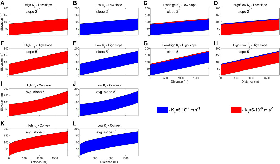
FIGURE 1. Hypothetical watershed configurations used in this study including four Longitudinal profiles combined with different assumptions on hydraulic conductivity (A–L). Low/high means that a layer with low Ks is resting on a layer of high Ks (C,G) and high/low refers to the opposite layering (D,H). The thickness of the upper layer in the layered experiments is 6 m.

All watersheds are represented by 25 cells of 80 m by 80 m (Slope length of 2 km and total area of 1.6 ⋅ 10⁵ m²). The soil column of each cell has a total depth of 85 m. In the previous work by Debolskiy et al. (2021), only one uniform slope (1°) was considered with a wider range of K_s (1 ⋅ 10^–5 to 1 ⋅ 10^–7 m⁻¹) as well as a shallower soil column (70 m) and bigger, but fewer grid cells (16 cells of 250 x 250 m). The modification of the prior setup is done to ensure that the minimum water table elevation at the uppermost cell in the watershed is not below the bottom of the soil column. Though WaSiM can handle situations when the water table is significantly below the bottom soil layer, it is not desirable for performance reasons. Zero soil moisture flux and geothermal heat flux of 0.085 W m⁻² boundary conditions are applied at the bottom of the soil column. At all the lateral boundaries of the watershed (including the ones perpendicular to the slope), a zero soil moisture flux condition is applied.

The model is forced with 30-min averages of near-surface air temperatures and total precipitation data. Following Debolskiy et al. (2021), we define two steady climates, a “cold” and a “warm” climate. The “cold” climate represents current conditions and consists of annual cycles of near-surface air temperature and precipitation that are derived from averaging spatial means across the Central Interior Alaska climate division (over the period 1970–2018) from the Climate Research Unit (CRU) dataset Harris et al. (2014). The mean annual air temperature is −4.8°C and annual precipitation is 340 mm y⁻¹. The CRU monthly climatology is then interpolated to the model time step (30 min) with the first four Fourier coefficients. A linear adjustment is applied to ensure a smooth transition at the end and the beginning of the following year. The annual cycle of the “warm” climate is obtained by adjusting the air temperature of the “cold” climate with a coefficient so that only negative temperatures are affected and the mean annual air temperature is increased by 7.5°C. By increasing the air temperature in this manner we ensure that the warm period temperatures and the timing of crossing 0°C are constant throughout the simulation period. This also means that the snowmelt starts at the same time and potential evapotranspiration is the same for both climates. The annual cycle of precipitation is assumed the same in both climates.

The “cold” and a “warm” climate are then used for pre-spinup and spinup and to derive a warming scenario that will lead to permafrost degradation. The model is initialized for pre-spinup with fully saturated soil below 10 m depth with uniform soil temperature distribution. The pre-spinup stage of simulations consists of 1,000 years of “warm” climate forcing. This is followed by a 1000-year spinup under “cold” climate forcing. First using the “warm” climate forcing prior to the “cold” climate forcing is essential to achieve realistic moisture distribution with in the soil as detailed in Debolskiy et al. (2021). We then finally apply a warming scenario defined by a linear transition between the “cold” and the “warm” steady climates over a period of 100 years beyond which the steady “warm” climate is continued for another 900 years.

3 Results

3.1 Water balance

During the 100-year-long transition period between the “cold” and “warm” climate all water balance components (normalized by precipitation) exhibit similar temporal patterns in all twelve watershed configurations (Figure 2). During the first 50–80 years into the transition a decrease in surface runoff is largely compensated by an increase in interflow, most prominently in cases with low K_s near the surface, (Figures 2B, C, E, G, J, L). In the following 20–50 years interflow and evapotranspiration drop considerably while freshly thawed soil is filling up with infiltrating water (ΔS increases). This is followed by a pronounced spike in interflow around the end of the transition period accompanied by decreasing ΔS. At the same time, very little baseflow generation occurs during the entire warm-up period.

FIGURE 2

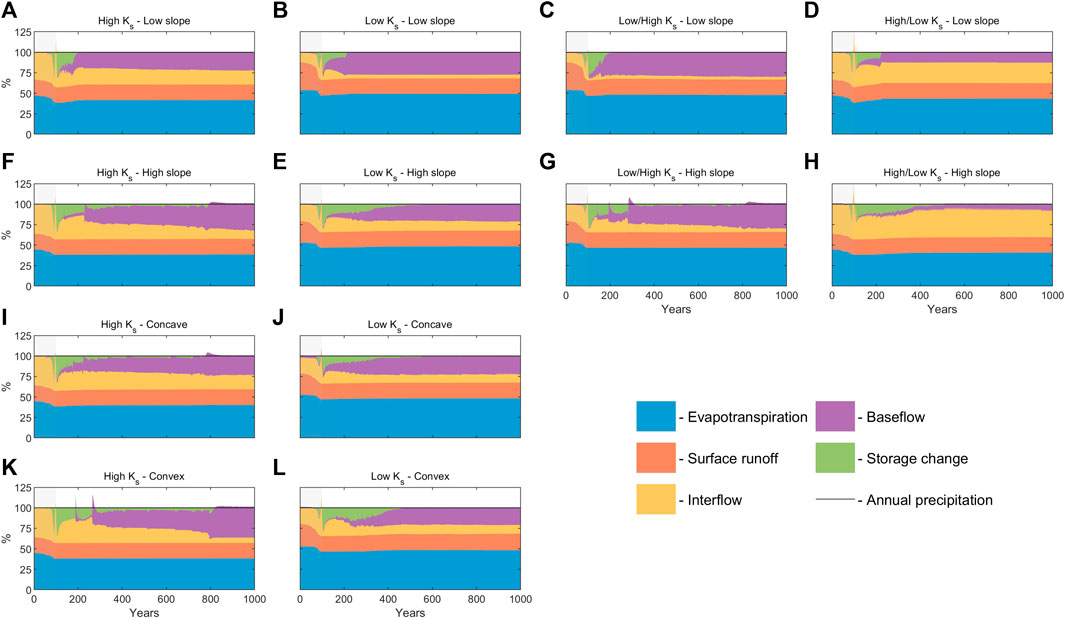
FIGURE 2. Simulated annual water balance components (stacked) in percent of annual precipitation (A–L). Grey shading marks the 100-year warm-up period. Configurations of the cases can be found in Figure 1.

After the warm-up period, the watersheds exhibit a period of variable length with increasing baseflow and subsurface water storage, the latter eventually approaching zero (Figure 2). While initially increasing during the 100-year-long warming-up period, interflow decreases continuously after 200 years of simulations while surface runoff exhibits an opposite pattern. The long-term increase in baseflow is largely compensated by decreases in interflow, while evapotranspiration and surface runoff tend to remain relatively constant. For watersheds with low slope (Figures 2A–D) the period of positive ΔS is shorter (100–150 years) than for high slope (Figures 2F–H) watersheds (400–700 years). In addition, watersheds with high slope and high saturated hydraulic conductivity (Figures 2F, G, I, K) exhibit a step-like behavior in the baseflow increase, which is most prominent in cases with convex topography and heterogeneous soil with higher hydraulic conductivity below with high slope (Figures 2G, K) where the “steps” result in negative ΔS for a few years at around 200 and 300 years after the beginning of warming scenario.

Initially, under the “cold” equilibrium conditions (prior to the warming scenario), total runoff consists almost entirely of surface runoff and interflow. The contribution of surface runoff to total runoff is generally lower for higher slopes and is not sensitive to the profile curvature of the watershed. Moreover, the relative surface runoff contribution is larger for the lower value of K_s (54%–74% of total runoff) than the higher value (34%–37%). In addition, the relative surface runoff contribution does not depend on the K_s of the lower layer in the heterogeneous cases. This is due to the fact that under cold equilibrium conditions, all hydrological activity is contained within the active layer and surface runoff/interflow separation is proportional to K (4). At the end of the warming scenario, all 12 watersheds exhibit similar values in the contribution of surface runoff to total runoff (30%–37%). This is due to the larger unsaturated zone which creates higher downward moisture flux and limiting surface runoff for any subsurface conditions and geometry. Evapotranspiration decreases by 4%–7% of total annual precipitation which is compensated by a roughly equal increase in runoff.

In contrast to the “cold” equilibrium conditions, where baseflow is almost never generated, after the warming period, baseflow represents a significant part of the total runoff (Table 1). The impact of slope on the contribution of baseflow to total runoff depends on K_s. Baseflow contribution to total runoff (as well as absolute amount) is higher for steeper slopes if K_s is high, however, when K_s is low—steeper slopes reduce baseflow. The latter is even more prominent in cases where near-surface soil has higher K_s. High/low K_s case with a steeper slope provides conditions most favorable for interflow generation. In the high K_s cases, the baseflow contribution has an inverse relationship with the watershed’s curvature while for the lower K_s curvature does not make a significant difference.

TABLE 1

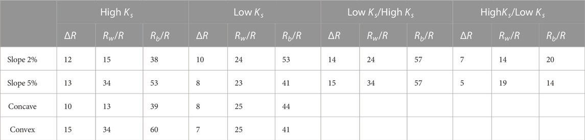
TABLE 1. Changes in total runoff (ΔR, %) at the end of the 1000-year warming scenario relative to the beginning, fractions (%) of winter runoff (R_w/R) and baseflow (R_b/R) of total runoff at the end of the 1000-year warming scenario. R_w and R_b prior to warming contribute ≤ 3% and ≤ 1% to total annual runoff respectively. Watershed configurations can be found in Figure 1.

With respect to seasonal variations in runoff components, we observe in all cases an increase in winter (period with negative air temperatures) runoff after 1,000 years (Figure 3). The contribution of winter runoff to total runoff is higher for steeper slopes and is lowest for concave curvature and homogeneously high K_s (Tab.1). When K_s of the near-surface soil is low (both in homogeneous and layered cases) a sharp peak (associated with high surface runoff) occurs during snowmelt season (Figures 3B, C, E, D, J, L) prior to the application of the warming scenario. However, when the watersheds have completely thawed there is less variability between the cases in runoff during snowmelt (which corresponds to lower surface runoff variability). When the near-surface K_s is high—a decrease in the late summer runoff associated with high interflow can be observed.

FIGURE 3

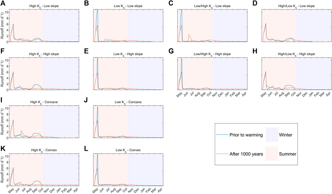
FIGURE 3. Simulated annual cycles of total runoff. Winter (October–April) and summer (May–October) periods are defined by negative and positive daily air temperatures, respectively (A–L). The watershed configurations can be found in Figure 1.

3.2 Soil temperature and moisture distribution

Initial soil temperature and moisture distribution (after the spinup) mostly depend on the average slope of the watershed (Figure 4; Figure 5; Figure 6) with the higher slope value having a deeper unsaturated zone and overall lower permafrost temperature. Under the same slope conditions, higher K_s also allows for a higher deficit in storage (Table 2) and lower soil temperatures in the upper part of the watersheds. After the 100-year-long warm-up period a shallow (4–6 m), mostly saturated talik is formed in the upper soil column while the permafrost in the head-water parts of the watersheds remains unsaturated. The drainage of this talik results in the aforementioned interflow peak after 100 years. After drainage of the talik, the soil column continues to thaw and in the low slope cases, the groundwater table rises within the first 100–150 years and resides in the upper 10 m of the soil column while thawing is continued downward. In the high slope case, while the permafrost table moves downwards with the same speed initially, 150–200 years after the onset of the warming the rate of thaw increases due to the lower moisture content and less phase change energy consumption by the phase change in the first few meters of the soil column.

FIGURE 4

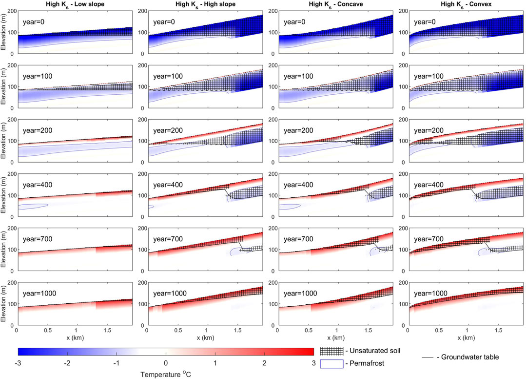
FIGURE 4. Soil temperature distribution and moisture saturation as a function of depth and distance from the mouth of the watershed for several time slices for four of the investigated watershed configurations with high K_s (Figures 1A, F, I, K).

FIGURE 5

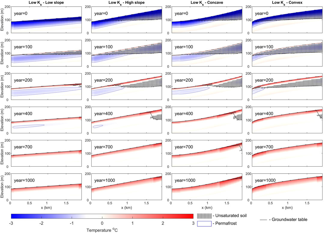
FIGURE 5. Soil temperature distribution and moisture saturation as a function of depth and distance from the mouth of the watershed for several time slices for four of the investigated watershed configurations with low K_s (Figures 1B, E, J, L).

FIGURE 6

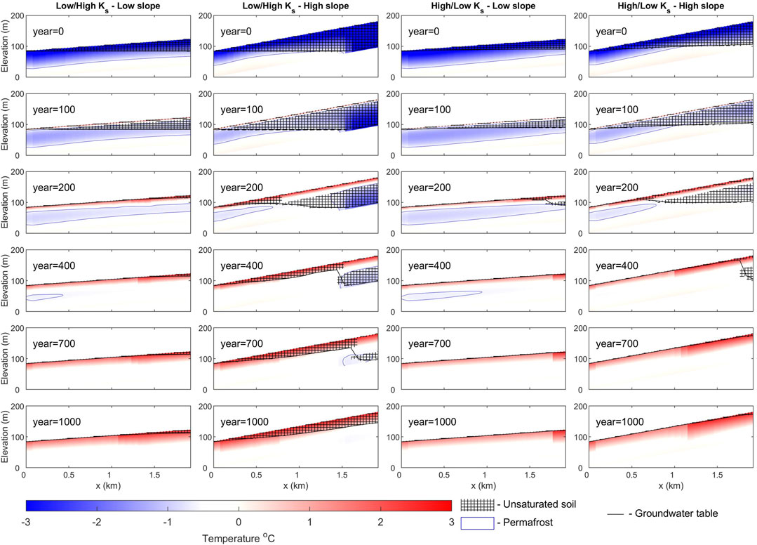
FIGURE 6. Soil temperature distribution and moisture saturation as a function of depth and distance from the mouth of the watershed for several time slices for four of the investigated watershed configurations with vertically heterogeneous K_s (Figures 1C, G, D, H).

TABLE 2

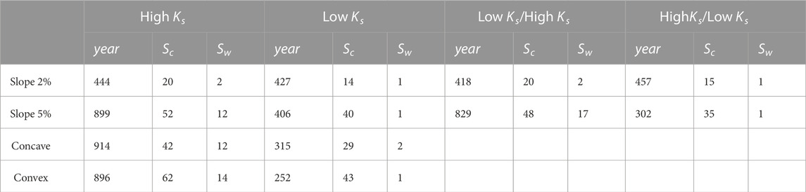
TABLE 2. Year after the start of the warming scenario when the permafrost has disappeared (year), and the volumetric fraction of the watershed that is unsaturated (%) immediately prior (S_s) and at the end of the 1000-year warming scenario (S_w). Watershed configurations and K_s values can be found in Figure 1.

The rate of thaw varies between the experiments (Table 2). Lower K_s, lower slope, as well as negative (convex) curvature, increase the rate of thaw over the entire 1000-year period of simulation. This is mostly due to the interplay between the energy spent on phase change and the dependency of thermal conductivity on moisture content. When a watershed cools, higher K_s in the lower soil, a steeper slope, and negative curvature allow for more efficient drainage of the aquifer beneath the newly formed permafrost. This, as well as a low “warm” state storage deficit, promotes more efficient cooling and watersheds and results in overall lower soil temperature when the watershed reaches “cold” equilibrium. During warming, although less moisture results in lower phase change energy expense, the effect of decreased thermal conductivity due to low water content and overall lower soil temperature results in slower permafrost thaw.

4 Discussion

Despite substantial differences in the set-up of the idealized watersheds, we find comparable ranges of overall runoff increase, transient responses for water-balance components, and watershed-wide soil moisture storage dynamics due to warming compared to Debolskiy et al. (2021). However, here we also consider different slopes and curvatures and find that the response of the watershed to the warming scenario depends on the watershed’s topography, but the dependence differs for high and low conductivity. When faster flow is enabled by the subsurface conditions watersheds with steeper slopes experience higher moisture deficit in the frozen state. This delays the watershed thawing but promotes higher baseflow and winter runoff. In watersheds with less permeable soils, this relationship is reversed. The latter is due to the fact that interflow generation scales with slope, while low K_s allow for high enough groundwater table for higher efficiency of this type of runoff generation. On the other hand, high K_s (through enhanced lateral subsurface flow) creates higher vertical moisture flux which “outcompetes” interflow generation during permafrost thawing. However, no matter the drainage configuration, we find an overall pattern of increased runoff, baseflow, and winter runoff accompanied by a decrease in evapotranspiration and surface runoff for the warming scenarios consistent with Debolskiy et al. (2021).

Similar to the setup in Debolskiy et al. (2021), our modeling framework is limited by a number of assumptions including, for example, strictly vertical and conductive heat transfer, lateral moisture transport occurring only in the saturated zone, identical soil properties apart from K_s, constant annual precipitation, increase in air temperatures only in the winter period, and constant vegetation type. The drawbacks and advantages of our experimental framework compared to similar studies (Frampton et al., 2011; 2013; McKenzie and Voss, 2013; Evans and Ge, 2017; Lamontagne-Hallé et al., 2018) have been thoroughly discussed in Debolskiy et al. (2021). However, it should be noted, that Lamontagne-Hallé et al. (2018) also observe higher influence of K_s (compared to slope) on groundwater discharge increase.

We note that our assumption of constant precipitation in the scenarios could introduce a potential bias into the simulation, especially in light of anticipated increases in precipitation with atmospheric warming and recent studies attributing the increase in annual runoff largely to increases in precipitation (Wang et al., 2021). Also, the impact of warming on vegetation (greening) is likely to influence water balances by increasing transpiration. However, we note, that our experiments aim to assess how permafrost thaw alone can shape the water balance of a watershed. Thus, we constructed our experiments deliberately in a way where we can eliminate the responses to other factors (changes in vegetation cover, changes in precipitation, potential evapotranspiration). Results indicate tangible impacts of permafrost alone on the water balance of our idealized watersheds.

Recent studies that employ WaSiM for modeling permafrost degradation effects on real watersheds’ water balance (e.g., Sun et al., 2020) agree broadly in the trajectories of water balance components demonstrated here. However, there are differences in soil moisture deficit dynamics between this study and Sun et al. (2020). There, the authors demonstrate that the soil moisture deficit is larger in a fully thawed watershed than in a frozen watershed, while our experiments reveal that frozen watersheds can have a higher soil water storage deficit than those fully thawed. This difference can be mainly explained by the fact that Sun et al. (2020) overestimates soil moisture storage for the “frozen” watershed since permafrost degradation is approximated by applying a model that does not calculate soil heat transfer. The initial conditions for both configurations (with and without heat transfer) are obtained from spinning up the model with heat transfer for 60 years from saturated soil. Although spinning up with a “cold” climate to obtain initial conditions is not uncommon (e.g., McKenzie and Voss, 2013; Jafarov et al., 2018) it results in frozen soil water that has not been able to escape the unconfined aquifer during permafrost aggradation.

5 Conclusion

Simulating the water balance of idealized watersheds underlain by permafrost in response to a warming scenario in winter (summer air temperature and annual precipitation remain unchanged), we demonstrate that one of the main consequences of the enhanced subsurface connectivity under warming is the decrease in near-surface soil moisture and the associated decrease in evapotranspiration. This decrease in evapotranspiration and the resulting increase in total runoff depends not only on the saturated hydraulic conductivity of the soil but also on the slope and curvature of the watershed. When K_s is high, steeper slopes promote a higher increase in runoff. When K_s is low, steeper slopes exhibit a lower relative increase in runoff. The profile curvature exhibits a reversed pattern—upwardly convex (negative curvature) cases exhibit higher runoff increases than concave. In addition, steeper watersheds take longer to fully thaw due to the interplay between phase change energy expenses and moisture-dependent thermal properties of the soils and the development of higher soil moisture deficit during freeze-up. Experiments with vertically heterogeneous K_s indicate that when the permeability of near-surface soil is high—greater interflow generation occurs during warming limiting baseflow and winter runoff contributions to the annual runoff. This effect is even more prominent for steeper slopes. However the overall pattern of watersheds behavior during warming in these experiments is similar to those with homogeneous K_s corresponding to K_s of the deeper soils in the layered configurations.

Data availability statement

The raw data supporting the conclusion of this article will be made available by the authors upon request, without undue reservation.

Author contributions

MD: Conceptualization, Formal Analysis, Investigation, Methodology, Visualization, Writing–original draft, Writing–review and editing. RH: Funding acquisition, Resources, Supervision, Writing–original draft, Writing–review and editing. VA: Conceptualization, Funding acquisition, Investigation, Methodology, Supervision, Writing–original draft, Writing–review and editing. VR: Funding acquisition, Resources, Supervision, Writing–review and editing.

Funding

The author(s) declare financial support was received for the research, authorship, and/or publication of this article. This research was funded by NSF grants ARC–1304271 and ARC–1832238, and by the Next-Generation Ecosystem Experiment (NGEE-Arctic) project. NGEE-Arctic is supported by the Office of Biological and Environmental Research in the DOE Office of Science. VA is supported by NSF Grant 2040240, the Interdisciplinary Research for Arctic Coastal Environments (InteRFACE) project through the Department of Energy, Office of Science, Biological and Environmental Research Program’s Regional and Global Model Analysis program and by NOAA project NA18OAR4590417.

Acknowledgments

The authors would like to thank D. J. Nicolsky for his support.

Conflict of interest

The authors declare that the research was conducted in the absence of any commercial or financial relationships that could be construed as a potential conflict of interest.

Publisher’s note

All claims expressed in this article are solely those of the authors and do not necessarily represent those of their affiliated organizations, or those of the publisher, the editors and the reviewers. Any product that may be evaluated in this article, or claim that may be made by its manufacturer, is not guaranteed or endorsed by the publisher.

References

Adam, J. C., and Lettenmaier, D. P. (2008). Application of new precipitation and reconstructed streamflow products to streamflow trend attribution in northern eurasia. J. Clim. 21, 1807–1828. doi:10.1175/2007JCLI1535.1

CrossRef Full Text | Google Scholar

Arp, C. D., Whitman, M. S., Jones, B. M., Kemnitz, R., Grosse, G., and Urban, F. E. (2012). Drainage network structure and hydrologic behavior of three lake-rich watersheds on the arctic coastal plain, Alaska. Arct. Antarct. Alp. Res. 44, 385–398. doi:10.1657/1938-4246-44.4.385

CrossRef Full Text | Google Scholar

Berezovskaya, S., Yang, D., and Kane, D. L. (2004). Compatibility analysis of precipitation and runoff trends over the large siberian watersheds. Geophys. Res. Lett. 31. doi:10.1029/2004GL021277

CrossRef Full Text | Google Scholar

Biskaborn, B. K., Smith, S. L., Noetzli, J., Matthes, H., Vieira, G., Streletskiy, D. A., et al. (2019). Permafrost is warming at a global scale. Nat. Commun. 10, 264. doi:10.1038/s41467-018-08240-4

PubMed Abstract | CrossRef Full Text | Google Scholar

Bring, A., and Destouni, G. (2011). Relevance of hydro-climatic change projection and monitoring for assessment of water cycle changes in the arctic. Ambio 40, 361–369. doi:10.1007/s13280-010-0109-1

PubMed Abstract | CrossRef Full Text | Google Scholar

Bring, A., Fedorova, I., Dibike, Y., Hinzman, L., Mård, J., Mernild, S. H., et al. (2016). Arctic terrestrial hydrology: a synthesis of processes, regional effects, and research challenges. J. Geophys. Res. Biogeosciences 121, 621–649. doi:10.1002/2015JG003131

CrossRef Full Text | Google Scholar

Connon, R. F., Quinton, W. L., Craig, J. R., and Hayashi, M. (2014). Changing hydrologic connectivity due to permafrost thaw in the lower liard river valley, nwt, Canada. Hydrol. Process. 28, 4163–4178. doi:10.1002/hyp.10206

CrossRef Full Text | Google Scholar

Debolskiy, M. V., Alexeev, V. A., Hock, R., Lammers, R. B., Shiklomanov, A., Schulla, J., et al. (2021). Water balance response of permafrost-affected watersheds to changes in air temperatures. Environ. Res. Lett. 16, 084054. doi:10.1088/1748-9326/ac12f3

CrossRef Full Text | Google Scholar

Déry, J., Stephen Stadnyk, T. A., MacDonald, M. K., and Gauli-Sharma, B. (2016). Recent trends and variability in river discharge across northern Canada. Hydrology Earth Syst. Sci. 20, 4801–4818. doi:10.5194/hess-20-4801-2016

CrossRef Full Text | Google Scholar

Evans, S. G., and Ge, S. (2017). Contrasting hydrogeologic responses to warming in permafrost and seasonally frozen ground hillslopes. Geophys. Res. Lett. 44, 1803–1813. doi:10.1002/2016GL072009

CrossRef Full Text | Google Scholar

Evans, S. G., Yokeley, B., Stephens, C., and Brewer, B. (2020). Potential mechanistic causes of increased baseflow across northern eurasia catchments underlain by permafrost. Hydrol. Process. 34, hyp.13759–2690. doi:10.1002/hyp.13759

CrossRef Full Text | Google Scholar

Fan, Y., Clark, M., Lawrence, D. M., Swenson, S., Band, L. E., Brantley, S. L., et al. (2019). Hillslope hydrology in global change research and earth system modeling. Water Resour. Res. 55, 1737–1772. doi:10.1029/2018WR023903

CrossRef Full Text | Google Scholar

Farquharson, L. M., Romanovsky, V. E., Kholodov, A., and Nicolsky, D. (2022). Sub-aerial talik formation observed across the discontinuous permafrost zone of Alaska. Nat. Geosci. 15, 475–481. doi:10.1038/s41561-022-00952-z

CrossRef Full Text | Google Scholar

Frampton, A., Painter, S., Lyon, S. W., and Destouni, G. (2011). Non-isothermal, three-phase simulations of near-surface flows in a model permafrost system under seasonal variability and climate change. J. Hydrology 403, 352–359. doi:10.1016/j.jhydrol.2011.04.010

CrossRef Full Text | Google Scholar

Frampton, A., Painter, S. L., and Destouni, G. (2013). Permafrost degradation and subsurface-flow changes caused by surface warming trends. Hydrogeology J. 21, 271–280. doi:10.1007/s10040-012-0938-z

CrossRef Full Text | Google Scholar

Hamon, W. R. (1960). Estimating potential evapotranspiration. Ph.D. thesis. Cambridge, Massachusetts: Massachusetts Institute of Technology.

Google Scholar

Harris, I., Jones, P., Osborn, T., and Lister, D. (2014). Updated high-resolution grids of monthly climatic observations – the cru ts3.10 dataset. Int. J. Climatol. 34, 623–642. doi:10.1002/joc.3711

CrossRef Full Text | Google Scholar

Holmes, R. M., Shiklomanov, A. I., Suslova, A., Tretiakov, M., McClelland, J. W., Spenser, R. G. M., et al. (2018). “River discharge,” in Arctic report card 2018. http://www.arctic.noaa.gov/reportcard (Accessed January 1, 2020).

Google Scholar

Jafarov, E. E., Coon, E. T., Harp, D. R., Wilson, C. J., Painter, S. L., Atchley, A. L., et al. (2018). Modeling the role of preferential snow accumulation in through talik development and hillslope groundwater flow in a transitional permafrost landscape. Environ. Res. Lett. 13, 105006. doi:10.1088/1748-9326/aadd30

CrossRef Full Text | Google Scholar

Lamontagne-Hallé, P., McKenzie, J. M., Kurylyk, B. L., and Zipper, S. C. (2018). Changing groundwater discharge dynamics in permafrost regions. Environ. Res. Lett. 13, 084017. doi:10.1088/1748-9326/aad404

CrossRef Full Text | Google Scholar

Liljedahl, A. K., Boike, J., Daanen, R. P., Fedorov, A. N., Frost, G. V., Grosse, G., et al. (2016). Pan-arctic ice-wedge degradation in warming permafrost and its influence on tundra hydrology. Nat. Geosci. 9, 312–318. doi:10.1038/ngeo2674

CrossRef Full Text | Google Scholar

McCauley, C. A., White, D. M., Lilly, M. R., and Nyman, D. M. (2002). A comparison of hydraulic conductivities, permeabilities and infiltration rates in frozen and unfrozen soils. Cold Regions Sci. Technol. 34, 117–125. doi:10.1016/S0165-232X(01)00064-7

CrossRef Full Text | Google Scholar

McKenzie, J. M., and Voss, C. I. (2013). Permafrost thaw in a nested groundwater-flow system. Hydrogeology J. 21, 299–316. doi:10.1007/s10040-012-0942-3

CrossRef Full Text | Google Scholar

Panyushkina, I. P., Meko, D. M., Shiklomanov, A., Thaxton, R. D., Myglan, V., Barinov, V. V., et al. (2021). Unprecedented acceleration of winter discharge of upper yenisei river inferred from tree rings. Environ. Res. Lett. 16, 125014. doi:10.1088/1748-9326/ac3e20

CrossRef Full Text | Google Scholar

Schulla, J. (1997). Hydrologische Modellierung von Flussgebieten zur Abschätzung der Folgen von Klimaänderungen. Ph.D. thesis. Zürich, Switzerland: ETH Zurich. doi:10.3929/ethz-a-001763261

CrossRef Full Text | Google Scholar

Schulla, J. (2019). Model description wasim (water balance simulation model). http://wasim.ch/downloads/doku/wasim/wasim_2019_en.pdf (Accessed December 31, 2019).

Google Scholar

Shiklomanov, A. I., and Lammers, R. B. (2011). “River discharge,” in Arctic report card 2011. http://www.arctic.noaa.gov/reportcard.

Google Scholar

Shiklomanov, A. I., Lammers, R. B., Lettenmaier, D. P., Polischuk, Y. M., Savichev, O. G., Smith, L. C., et al. (2013). “Hydrological changes: historical analysis, contemporary status, and future projections,” in Regional environmental changes in siberia and their global consequences (Berlin, Germany: Springer), 111–154.

CrossRef Full Text | Google Scholar

Stuefer, S., Yang, D., and Shiklomanov, A. (2011). “Effect of streamflow regulation on mean annual discharge variability of the yenisei river,” in Cold regions hydrology in a changing climate. General assembly (25th: 2011. Editors I. A. of Hydrological Sciences, D. Yang, P. Marsh, A. Gelfan, I. U. of Geodesy, and V. Geophysics (Melbourne (Wallingford, Oxfordshire, UK: IAHS Press).

Google Scholar

Sun, A., Yu, Z., Zhou, J., Acharya, K., Ju, Q., Xing, R., et al. (2020). Quantified hydrological responses to permafrost degradation in the headwaters of the yellow river (hwyr) in high asia. Sci. Total Environ. 712, 135632. doi:10.1016/j.scitotenv.2019.135632

PubMed Abstract | CrossRef Full Text | Google Scholar

Swenson, S. C., Clark, M., Fan, Y., Lawrence, D. M., and Perket, J. (2019). Representing intrahillslope lateral subsurface flow in the community land model. J. Adv. Model. Earth Syst. 11, 4044–4065. doi:10.1029/2019MS001833

CrossRef Full Text | Google Scholar

Tan, X., and Gan, T. Y. (2015). Nonstationary analysis of annual maximum streamflow of Canada. J. Clim. 28, 1788–1805. doi:10.1175/JCLI-D-14-00538.1

CrossRef Full Text | Google Scholar

Tananaev, N., Teisserenc, R., and Debolskiy, M. (2020). Permafrost hydrology research domain: process-based adjustment. Hydrology 7, 6. doi:10.3390/hydrology7010006

CrossRef Full Text | Google Scholar

Tananaev, N. I., Makarieva, O. M., and Lebedeva, L. S. (2016). Trends in annual and extreme flows in the lena river basin, northern eurasia. Geophys. Res. Lett. 43 (10), 772. doi:10.1002/2016GL070796

CrossRef Full Text | Google Scholar

Walvoord, M. A., and Kurylyk, B. L. (2016). Hydrologic impacts of thawing permafrost—a review. Vadose Zone J. 15, 1–20. doi:10.2136/vzj2016.01.0010

CrossRef Full Text | Google Scholar

Wang, P., Huang, Q., Pozdniakov, S. P., Liu, S., Ma, N., Wang, T., et al. (2021). Potential role of permafrost thaw on increasing siberian river discharge. Environ. Res. Lett. 16, 034046. doi:10.1088/1748-9326/abe326

CrossRef Full Text | Google Scholar

Woo, M.-K., Kane, D. L., Carey, S. K., and Yang, D. (2008). Progress in permafrost hydrology in the new millennium. Permafr. Periglac. Process. 19, 237–254. doi:10.1002/ppp.613

CrossRef Full Text | Google Scholar