 Sasha Z. Leidman
 Åsa K. Rennermalm
 Rohi Muthyala1
 S. McKenzie Skiles
- 1Department of Geography, Rutgers, The State University of New Jersey, Piscataway, NJ, United States
- 2Department of Geography, University of Utah, Salt Lake City, UT, United States
- 3Department of Earth Sciences, Dartmouth University, Hanover, NH, United States
On the surface of the Greenland Ice Sheet, the presence of low-albedo features greatly contributes to ablation zone meltwater production. Some of the lowest albedo features on the Ice Sheet are water-filled supraglacial stream channels, especially those with abundant deposits of consolidated cryoconite sediment. Because these sediments enhance melting by disproportionately lowering albedo, studying their spatial extent can provide a better understanding of Greenland’s contribution to global sea level rise. However, little is known about the spatial distribution of supraglacial stream sediment, or how it changes in response to seasonal flow regimes. Here, we surveyed a supraglacial stream network in Southwest Greenland, collecting imagery from seven uncrewed aerial vehicle (UAV) flights over the course of 24 days in 2019. Using Structure-from-Motion-generated orthomosaic imagery and digital elevation models (DEMs), we manually digitized the banks of the supraglacial stream channels, classified the areal coverage of sediment deposits, and modeled how the terrain influences the amount of incoming solar radiation at the Ice Sheet surface. We used imagery classified by surface types and in-situ spectrometer measurements to determine how changes in sediment cover altered albedo. We found that, within our study area, only 15% of cryoconite sediment was consolidated in cryoconite holes; the remaining 85% was located within supraglacial streams mostly concentrated on daily inundated riverbanks (hereafter termed floodplains). Sediment cover and stream width are highly correlated, suggesting that sediment influx into supraglacial drainage systems widens stream channels or darkens previously widened channels. This reduces albedo in floodplains that already receive greater solar radiation due to their flatness. Additionally, the areal extent of stream sediments increased in August following seasonal peak flow, suggesting that as stream power decreases, more sediment accumulates in supraglacial channels. This negative feedback loop for melting may delay Greenland’s runoff to the latter end of the melt season. This study shows in unprecedented detail where and when sediment is deposited and how these deposits potentially impact the Ice Sheet surface energy balance. These findings may allow for better prediction of how supraglacial floodplains, and the microbiomes they contain, might change in response to increased melting.
1 Introduction
Greenland Ice Sheet mass loss is a major contributor to global sea level rise. Between 2002–2017 Greenland contributed 267.77 ± 8.68 Gt yr−1 to sea level rise (Zou et al., 2020), corresponding to 46% of total Arctic land ice contributions (Box et al., 2018). Over half of the observed ice loss results from negative surface mass balances (Shepherd et al., 2020). This mass loss process is exacerbated by the prevalence of low albedo features on the Ice Sheet surface including supraglacial streams and sediment (Tedesco et al., 2016; Ryan et al., 2018). Supraglacial stream drainage networks form in the ablation zone of glaciers around the world (Holmes, 1955; Ferguson, 1973; Marston, 1983; Smith et al., 2015; Watson et al., 2016; Kingslake et al., 2017; Ryan et al., 2018; Lu et al., 2020). These supraglacial stream networks form a series of supraglacial lakes, meandering rivers, and floodplains (flat, sediment-covered regions along the stream banks that are often diurnally inundated with meltwater) as meltwater flows toward moulins (Rennermalm et al., 2013a; Karlstrom et al., 2013; Chu, 2014; Leidman et al., 2021a).
On the Greenland Ice Sheet, supraglacial streams cover between 2 and 7% of the ablation zone surface (Ryan et al., 2018; Lu et al., 2021). Despite their relatively low spatial coverage, supraglacial streams explain 12% of Greenland’s albedo variability in the ablation zone (Ryan et al., 2018). One reason for this is that supraglacial streams consolidate low albedo (0.09) sediment along their beds (Ryan et al., 2018; Leidman et al., 2021b). Sediment is transported onto the surface of the Greenland Ice Sheet by windborne transport from local proglacial moraines and valleys (Bøggild et al., 2010; Nelson et al., 2014; Humbert et al., 2020) as well as, but to a lesser extent, accumulation of fine dust particles from long-range sources such as Asia (Bory et al., 2002; Bory et al., 2003), surface melting of ice containing outcroppings of Pleistocene era long-range dust (Bøggild et al., 2010; Cooper et al., 2018), landslides (Svennevig, 2019), and thrust faulting (Moore et al., 2010). Once on the Ice Sheet, sediment stays distributed on the surface, melts into cryoconite holes, or washes into supraglacial streams (Leidman et al., 2021a).
Surface impurities from algae and sediment can be widespread in regions such as the so-called Dark Zone in Southwest Greenland resulting in algae-rich regions having albedo values ∼0.4 lower than clean ice (i.e., ice with a minimal amount of surface impurities) regions (Cook et al., 2012; Yallop et al., 2012; Stibal et al., 2017; Williamson et al., 2018; Wang et al., 2020). As more of the Dark Zone becomes snow-free for longer periods due to climate change, algal blooms growing on the surface also increase and accelerate melting (Wang et al., 2018; Ryan et al., 2019; Wang et al., 2020). Distributed sediments on the ice surface often consolidate and, due to their dark coloration, absorb solar radiation and melt into the ice, forming cryoconite holes roughly 0.15–0.30 m deep (Bøggild et al., 2010). Sediment within cryoconite holes harbors cyanobacteria, algae, and micro-invertebrates (Uetake et al., 2016; Uetake et al., 2019). As these organisms grow, they wrap around sediment grains and form extracellular polymeric substances causing grains to clump together into granules (Hodson et al., 2010; Nagar et al., 2021). As a result, cryoconite can have organic contents of >6% dry weight at higher Ice Sheet elevations where cryoconite holes have more time to develop (Stibal et al., 2010).
Once cryoconite holes form, surface albedo may be 0.6 higher than areas with distributed sediment as the bottom of the cryoconite hole is largely shaded from direct sunlight due to the hole geometry and ice lids coving the holes after nighttime freezing (Bøggild et al., 2010). However, sediment granules can flush out of cryoconite holes during heavy melt events (often associated with cloudy conditions or rainfall; Takeuchi et al., 2018; Tedstone et al., 2020; Muthyala et al., 2022) and deposit in supraglacial streams (Leidman et al., 2021b). The similar granular structure and composition of sediment found in supraglacial streams also indicates that it predominantly originates from these cryoconite holes (Bøggild et al., 2010).
Supraglacial water bodies (lakes, streams) have a significantly lower albedo than the surrounding clean ice (0.21 for water bodies compared to 0.55 for clean ice) and, as such, disproportionately contribute to negative surface mass balances (Pope et al., 2016; Ryan et al., 2018). Previous research using synoptic numerical models show that for shallow streams (0.5 m depth), 38% of the incoming spectrally integrated solar radiation is absorbed by the bed compared to 51% by the water column (Bray et al., 2017). As a result, for terrestrial streams, dark sediment along the streambed can facilitate enough energy absorption to increase water temperatures by over 2°C (Bray et al., 2017). Isenko et al. (2005) observed that this process also occurs in supraglacial streams resulting in stream temperatures up to 0.4°C when sediment was present. Energy absorbed by supraglacial stream sediment may be partially re-radiated back to the atmosphere or exported from the glacier’s terminus before contributing to increased melting. However, the long transport distance between the absorption and export locations and the similar hydraulic properties of these systems to terrestrial rivers (Marston, 1983; Smith et al., 2015; Gleason et al., 2016; Muthyala et al., 2022) suggests that much of the solar energy absorbed by sediment goes towards increasing melt rates. The highly turbulent flow characteristics of supraglacial streams (Gleason et al., 2016) would also facilitate a more efficient transfer of energy to the ice for melting. The fact that supraglacial streams display extensive incision compared to the background ablation rates (Ferguson, 1973; Karlstrom et al., 2013; Leidman et al., 2021a) also points to an efficient transfer of energy to the bed. While this incision can lead to shadowing of the stream channel (Leidman et al., 2021b), this effect is only significant in areas of high relief (such as near immediately upstream of moulins). Despite this incision induced shadowing, hydrological modeling of supraglacial stream meandering indicates that the majority of the melt energy goes towards lateral rather than vertical melting thereby continuing the exposure of the stream bed to direct solar radiation (Karlstrom et al., 2013). In this study, we therefore assume that all energy absorbed due to changes in albedo translate to changes in meltwater production.
This study investigates how sediment within supraglacial stream networks change throughout the melt season and postulate how it might impact albedo in response to changing meltwater inputs. We use repeat photography from uncrewed aerial vehicle (UAV) flights to classify supraglacial streams and sediment in a supraglacial catchment in Southwest Greenland. In total, seven classified imagery mosaics were used to determine how sediment cover changes throughout the stream length and melt season. Additionally, we use digital elevation models (DEMs) derived from the UAV imagery and in-situ hyperspectral measurements of various surfaces to determine the amount of incoming solar radiation exposure for each surface class; bare ice, water, stream sediment, and cryoconite holes. We compare results with stream discharge to examine whether sediment cover is dependent on stream power and, if so, discuss how sediment might impact the input of meltwater and nutrients to the subglacial environment.
2 Data
2.1 UAV imagery collection
To investigate the intra-seasonal variation of supraglacial stream sediment distribution, we conducted repeat UAV flights with a DJI Phantom 3 or a DJI Mavic 2 Pro over a single supraglacial catchment in Southwest Greenland (67.15⁰N, 50.00⁰W) (Figure 1). In total, seven flights were conducted (July 22, August 2, 4, 7, 11, 14, and 15, 2019) (Table 1). All imagery was collected within 3 h of solar noon. The DJI Phantom 3 was mounted with an 18 megapixel FC3610 camera whereas the Mavic 2 Pro was mounted with a 17 megapixel L1D-20c camera. All images were collected at a maximum height of 60 m from the surface and had at least 80% image overlap. Markers were placed around the study site to use as ground control points including orange plastic trays (0.35 x 0.25 m) (Supplementary Figure S1), orange painted rocks (∼0.1 m diameter), and red tarps with black X’s to demark the center point (1.5 x 1.5 m).
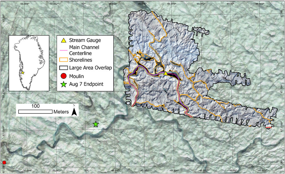
FIGURE 1. Map of the study site with UAV imagery from 22 July 2019 clipped to the large area overlap footprint. Orange lines show the location of manually digitized shorelines and the pink line indicates the centerline of the main channel. The location of the stream gauge used to measure water depth throughout the observation period, the furthest downstream location of the August 7th observed main channel, and the moulin for the main channel are shown as a yellow triangle, a green star, and a red circle respectively. The inset map shows the location of the field site in southwestern Greenland. Background imagery is a Maxar Technologies image obtained from Google Earth collected on July 24, 2012 overlain on the ArcticDEM (Polar Geospatial Center et al., 2018). Because the time offset between the background image (2012) and the data collection (2019), the movement of the ice has shifted the channel location and the Aug 7 Endpoint and moulin are outside the 2012 channel.
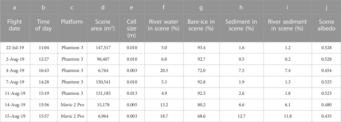
TABLE 1. Statistics of the spatial distribution of sediment and water within each flight scene including the date (a) and average time the images were collected (West Greenland local time) (b), UAV platform (c), area of the UAV scene footprint (d), structure-from-motion output cell size (e), the percent of the scene covered by river water rivers (includes both river beds covered by sediment and clear ice) (f), the percent of the scene covered by bare ice (g), the percent of the scene covered by sediment (includes sediment on bare ice and in the river) (h), and the percent of the scene where rivers are covered by sediment. Albedo was calculated as the weighted average of the extent of the scene covered in river water (f minus i) and bare ice (g) using and albedo value of 0.26 and 0.55 respectively from Ryan et al. (2018) as well as the extent of the scene covered in sediemnt using an albedo of 0.07 derived from Figure 2.
2.2 UAV imagery processing
The imagery collected from each of the seven UAV flights was georeferenced and processed using Agisoft Metashape Pro v1.6.5 Structure-from-Motion software to create high quality dense point clouds that were then converted to DEM and orthomosaic images. Outputs were exported at their maximum raster resolution (0.026 ± 0.016 m for the DEMs and 0.008 ± 0.004 m for the orthomosaics; Table 1). All DEMs and orthomosaics were georeferenced to the UTM 22 N projection, a conformal, shape-preserving projection with minimal distortion in this area. Due to logistical challenges of collecting data on the Ice Sheet, imagery coverage varied from 0.007 to 0.151 km2 (Supplementary Figures S2–S8; Table 1).
2.3 Surface reflectance data
To relate changes in the extent of sediment and stream channels to changes in surface energy balance of the field site, we created an empirical relationship between water depth, sediment cover, and broadband reflectance collected with an Analytical Spectral Devices (ASD) Fieldspec4 Pro spectrometer. The ASD contiguously samples the spectral range 350—2500 nm for each measurement. In total, 41 ASD measurements were collected, all of which were under consistent illumination conditions within 2 h of solar noon. Sampling sites were selected quasi-randomly throughout the area of overlapping flight footprints (Supplementary Figure S9) in order to measure a range of different surfaces with varying sediment coverage and water depths. The spectral reflectance at each location was calculated by taking the ratio between the average of ten upwelling solar radiance measurements of the ground surface and the average of ten upwelling solar radiance measurements of a Spectralon panel reflector. Spectral irradiance was used to calculate the spectrally weighted broadband reflectance value. Co-located ground surface images were taken in tandem with ASD measurements. Surface images were collected in triplicate with a RICOH WG-30W 5-megapixel digital camera.
Surface images were cropped using a centered circular geometry to match the area covered by the 7.5° viewing angle of the spectrometer at the height of the camera during image capture. Cropped images were then converted to black and white images in Adobe Photoshop v22.5.1. All images were manually inspected to ensure that they matched the expected spectrometer coverage and areas of contiguous sediment patches that displayed speckling or glare artifacts were manually edited. The proportion of black versus white pixels was used to determine the average sediment cover for the triplicate images. Sediment cover could be obtained this way due to the high visual difference between the clean ice (converted to white) and dark sediment (converted to black). All images were taken within 2 h of solar noon under similar cloud conditions. Clean ice and dark sediment were spectrally quite distinct and we determined that any errors from slight tilting of the camera were likely significantly higher than any errors associated with illumination. Reflectance was plotted against sediment cover and fitted with a least-squares best fit exponential trend line (Figure 2). The 100% sediment cover intercept of this relationship was used to determine the reflectance of sediment observed in UAV imagery, which was found to be 0.07 (Figure 2).
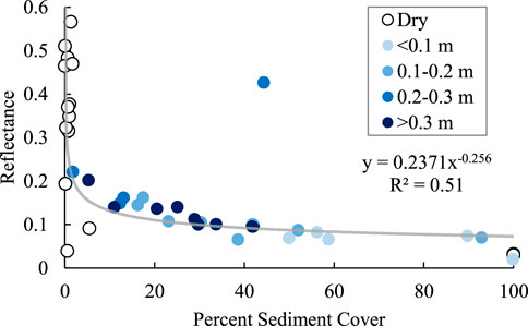
FIGURE 2. Scatterplot of reflectance values for each of ASD measurement and the sediment cover derived from classified handheld imagery of the ground surface within the ASD field of view. Colors indicate the water depth of the measurement site. The least-squares trendline was used to determine the albedo of 0.07 for 100% sediment cover where y is reflectance, and x is the percent sediment cover. R2 is the coefficient of determination of the trendline.
2.4 Water-level and runoff data
Stream water pressure was measured with a Solinst Levellogger pressure transducer placed in a RACO-2 metal project box filled with rocks with conduit holes knocked out to allow water to easily flow into the box. The box was anchored to a PVC pole, which was drilled into the thalweg of the main stream channel (denoted as the stream gauge in Figure 1). The Levellogger continuously measured water pressure every minute between July 13th and August 10th, 2019 (Supplementary Figure S10). Water level was calculated by correcting water pressures for atmospheric pressure. Atmospheric pressure was measured using a Solinst Barologger fixed in place 2 m above the ice on the shore of the largest channel within the study area (hereafter termed the main channel). Manual measurements of water depth were recorded with a meter stick periodically throughout the field season to determine if any measurement drift was present and to correct for systematic instrumentation error. The metal conduit box was thick enough to prevent accelerated melting of the underlying bed faster than the surrounding ablation rate, hence the logger stayed stationary relative to the bed throughout the measurement period. Additionally, stream discharge was measured with a Sontek Flowtracker2 Acoustic Doppler Velocimeter immediately upstream of the Levellogger. In total, 33 measurements of discharge were recorded throughout the study period and used to produce a rating curve to convert water level measurements to discharge throughout the observation period (Supplementary Figure S11).
Additionally, we examined runoff estimates gathered from the Modéle Atmosphérique Régional (MAR) regional climate model version 3.11.5 (Fettweis et al., 2017) in order to extend the runoff record to the length of the UAV observation period. Average modelled daily runoff over the course of the observation period was calculated from the four 15 km grid cells closest to our study area (Supplementary Table S1). The center points of the grid cells were 10.8 ± 2.2 km (mean ± standard deviation) from the 7-Aug endpoint, had an average elevation of 627 m and average ice coverage of 74%. Runoff values were highly correlated with stream discharge measurements (p<<0.01, Supplementary Figure S11). This data was used to compare changes in reflectance of the stream system to changes in runoff (Figure 7).
3 Methodology
3.1 Feature mapping and network analysis
The shorelines for all streams at least 0.1 m wide from all seven flights were manually digitized using ArcGIS Pro v2.7.2. While flights were taken at different times of day (Table 1) and different water levels, analysis of stream water level showed that water heights were all within 30% of each other. Importantly, all of the images were collected when water level was high enough to fully inundate the observed floodplains. Channel walls were relatively steep outside of the floodplain boundary and therefore the variability in water level for the different image acquisition times resulted in insignificant variability in stream width and only a minimal impact on our analysis of sediment extent. Channel centerlines were found by calculating Euclidean distance from the shorelines and running a flow accumulation algorithm on the distance raster to the 7-Aug end point. The centerlines were inspected manually and proved to be more accurate than those generated by the ArcGIS Pro’s centerline tool.
The generated centerlines were used to determine how sediment cover on the stream bed changed along the length of the main channel. We quantified sediment cover for each zone. Zones subdivided the stream area every 1-m along the stream centerline from the 7-Aug endpoint (the furthest observed downstream location) to the August 11th start-point (the furthest observed upstream location). To create these zones, we generated points every 0.2 m along the stream centerlines. Then, the Network Analyst Closest Facility tool in ArcGIS was used to find the distance along the centerline of each point to the endpoint for the corresponding imagery from that flight date. The path distances determined for each point were adjusted so that they all represented the distance to the 7-Aug endpoint. We then used these points to create 1-m zones that spanned the width of the stream channel and extended 1-m along the centerline of each UAV scene. Finally, we applied an inverse distance weighting (IDW) algorithm on the network distance point values. The resulting interpolated output raster, clipped to the stream extent of the hand digitized stream shorelines, was then used to find 1-m contours. These contours were used as the boundaries for the 1-m zones used for quantifying sediment cover along the stream length.
Additionally, the 1-m zones were used to analyze how elevation, stream width, water-surface slope, and exposure to sunlight changed as you moved up the main stream channel. Average elevation of each 1-m zone was calculated using zonal statistics on the UAV derived DEM. Elevation data was also extracted to each centerline point and a linear regression was fitted to each point contained within each 1-m zone to determine the water surface slope (Supplementary Figure S12). The average width of the channel for each zone was determined by creating a Euclidean distance raster from the channel shorelines and doubling the resulting extracted values at the center-point locations. Average width for each 1-m zone was therefore calculated as twice the distance to the shorelines averaged over all the center-points within the 1-m zone.
3.2 Surface feature classification
The glacier surface observed in each UAV image was classified into three types: bare-ice, sediment, and water bodies, where sediment could cover either ice or stream. The classification was achieved by first applying a Maximum Likelihood supervised classification algorithm in ArcGIS Pro to each orthomosaic image to identify stream water, bare-ice, and sediment. Twenty-five training polygons were used for each of the three classes of each image totaling 600 polygons averaging 1.0 m2 in area each. This is the same method for classifying sediment areas as published by Leidman et al. (2021a) and, since each classification was made using training polygons from the same image, this method effectively accounts for variable solar illumination of the different mosaic images. The location of each classified pixel was then analyzed to determine whether it was found within or outside of the manually digitized stream extent. Visual inspection showed that while the classification of sediment areas was highly accurate, this process led to an overestimation of water outside of streams as well as pixels within the streams classified as bare-ice. This was likely due to the spectral similarities between bare-ice and water in RGB imagery as well as variable illumination throughout the scene due to shadows and scattered clouds. To account for this error, we used the manually digitized stream extent to convert all pixels identified as bare-ice within a stream channel to water pixels and all pixels classified as water outside of the stream as bare-ice. This correction needed to be applied to roughly 30% of stream pixels and 7% of non-stream pixels but resulted in a classification that better matched observations. Zonal statistics were then used to determine the average sediment concentration for each 1-m zone along the channel centerlines.
3.3 Influence of terrain on solar irradiance
In our study area, the walls of deeply incised supraglacial stream can cast shadows the Ice Sheet surface and cause large variability in incoming solar radiation (Leidman et al., 2021b). To examine how shadowing from local topography affects the radiation exposure of sediment within stream systems compared to sediment within cryoconite holes, we used ArcGIS Pro’s Area Solar Radiation tool (Kausika and van Sark, 2021) and the Structure-from-Motion DEM to model irradiance for each pixel within the study area over the course of a 24-h clear-sky day. Specifically, solar irradiance was calculated every 15 min for 24-h using the DEM retrieved on July 22nd as well as a transmissivity value of 0.545 which is representative for the atmospheric conditions in this area (van den Broeke et al., 2008). The distribution of solar radiation values for each surface cover class inside and out of the stream extent (i.e. sediment, ice, and water; section 3.2) were examined. This allowed us to determine if sediment inside the stream received more incoming solar radiation than sediment consolidated on bare-ice. Incoming solar radiation was also correlated with the average stream width of each 1 m zone, however the relationship is weak (Supplementary Figure S13).
3.4 Meteorological data
Daily averaged wind speeds were gathered from the PROMICE Automatic Weather Station network (Fausto et al., 2021) for KAN_L. KAN_L is located about 7 km south of our study site at 67.0955 N, 49.9513 W with an elevation of 670 m. Wind speed is measured at approximately 3.1 m above the ice with a R. M. Young 05103 wind monitor every 10 min. Trends in wind speed data were used to determine if local weather conditions potentially had an impact on sediment deposition rates within the observation period.
4 Results
4.1 Stream geometry
In the study area, the main channel was 4.6 ± 2.6 m wide (mean ± standard deviation), with a maximum width of 17 m across (including diurnally inundated floodplains). Tributaries were, on average, one-third the size of the main channel with widths weighted by mapped stream length of 1.7 ± 2.2 m (mean ± standard deviation) wide with a median width of 0.8 m. There were no endorheic lakes within the study area besides a few small melt pools (less than 1-m wide). Instead, the supraglacial hydrology within the study area was dominated by streams. Supraglacial streams covered 8.4 ± 0.4% (mean ± standard deviation) of the large scene area (hereafter defined as the overlapping region of the four orthomosaics with the widest coverage, Figure 1 and Table 2). This is greater than the 2% reported by Ryan et al. (2018) and 1–2% reported by Bøggild et al. (2010) for northeast Greenland as well as the seasonal maximum supraglacial river area fraction of 4.5% reported by Lu et al. (2021) for the Devon Ice Cap.
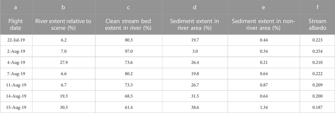
TABLE 2. Statistics for the coverage of the streams within the UAV scenes derived from manually digitized shorelines (b) as well as the relative coverage of clean ice (c) and sediment within (d) and outside of (e)observed in each flight scene. Stream albedo was calculated as the weighted average of columns c and d using albedo values of 0.24 and 0.07 respectively.
4.2 Sediment coverage
Within the large area scene (overlapping stream area for the four UAV scenes with the largest coverage), sediment covered 26.5 ± 3.3% (mean ± standard deviation) of the stream bed (Table 1, range 23–31%). Sediment in streams on average comprised 85% of the areal coverage of all sediment visible to the UAV within the study area. In total, sediment covered 2.6% of the large scene area on average and, although not measured, the granule size of sediment within the streams appeared similar to that found in cryoconite holes. Sediment coverage along the main channel reached up to 91% cover within the 1-m cross-sectional contour zones (Figure 3A). While sediment cover within the stream increased throughout the observation period, no consistent trend was observed as a function of distance to the endpoint. Instead, changes in sediment cover within the main channel ranged from -3.0 to 2.6% per day (standard deviation = 0.72% d−1) (Figure 3B). Within the small scene area (overlapping stream area for all seven scenes), sediment concentrations decreased from July 22nd to August 4th and then steadily increased thereafter at a rate of 0.75% per day on average (10% in total) (Figure 4, Supplementary Figure S14). The change was smaller for the large scene area where the August sediment cover only increased by 0.09% per day. Sediment outside of the stream system (mainly cryoconite holes) within the large scene area showed a much lower trend increasing in areal coverage by only 0.02% per day in August.
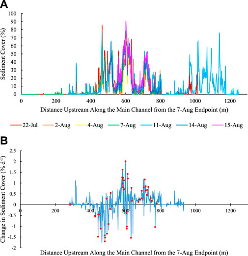
FIGURE 3. (A) Sediment cover within each 1-m zone along the main channel for each flight. Distances are relative to the flow path distance to the 7-Aug stream endpoint (c.f. Figure 1). (B) The rate of change in sediment cover (slope of the linear regression of sediment cover, % d−1) for each 1-m zone of the main channel with at least three observations. Sections of the stream where the change in sediment cover was statistically significant (p<0.05), are indicated with red dots. On average, sediment cover of the main channel increased by 0.07% per day.
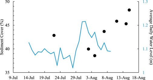
FIGURE 4. Sediment cover of the main channel between 582 and 757 m from the 7-Aug endpoint (c.f. Figure 1). This stream reach corresponds to the section of the main channel where all seven flights overlap. The blue line indicates the average daily water level recorded within the main channel. The black dots indicate the percentage of the stream channel covered by sediment for each flight.
Sediment cover also seemed to have an impact on the roughness of the stream bed. Areas of total sediment cover were uniformly flat whereas areas of patchwork sediment cover displayed a rougher ice surface with hummocks and holes multiple centimeters deep where sediment congregated. While not directly measured, this geometry seemed constant throughout the observation period and likely did not have an effect on the seasonal change in sediment cover. Areas near the thalweg that were covered by water throughout the night had smoother bed surfaces than areas with diurnal inundation therefore this process likely had a minimal impact on the roughness of the streambed.
4.3 Relationship between width, sediment cover, and solar radiation
Analysis of the spatial distribution of sediment floodplains revealed that wider sections of the stream contained more sediment than narrower sections (p-value << 0.01, Figure 5, Supplementary Figure S15). As a result, stream sections with above average width were 21% covered in sediment whereas stream sections with below average width were only 2% covered in sediment on average. The relationship between stream width and sediment cover persisted throughout the observation period (Supplementary Figure S15). A statistically significant relationship was also present between channel slope and sediment cover (p < 0.01), however the lower reliability of the elevation data from the structure-from-motion DEMs used to derive slope gives us limited confidence in this relationship (Supplementary Figure S12).
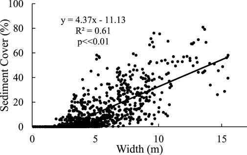
FIGURE 5. Relationship between stream width and average sediment cover for each meter of the main channel that falls within the small scene where all seven flights overlaps.
The wider widths and flatter terrain of sediment covered areas of the stream resulted in fewer shadows precluding incoming solar radiation from reaching the surface. As a result, sediment within the river system on July 22nd, on average, received 7.8% more incoming solar radiation compared to sediment outside of the stream (Figure 6, Supplementary Figure S16).
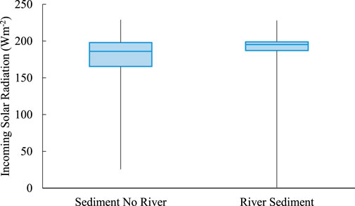
FIGURE 6. Box plot of incoming solar radiation for sediment in the stream (right) and outside of the stream (left). The difference in the average values of the two distributions was 14 Wm−2. This is equivalent to an increase in incoming solar radiation of 7.8% for sediment in the stream.
4.4 Change in albedo over the melt season
Albedo of the study area was calculated using values for bare-ice and shallow water albedo from the literature (0.55 and 0.26 respectively, Ryan et al., 2018) as well as measured reflectance values for cryoconite sediment (0.07, Figure 2) weighted using the spatial coverage for each class from the classified imagery. The maximum albedo of the large scene area before peak melt (July 22nd) was 0.522. The trend in albedo after peak melting was determined by the linear regression of the albedo values of the three August flights. The trend in albedo before peak melting was determined as the linear regression between the July 22nd albedo and the August 1st albedo extrapolated from the aforementioned post-peak trend. After peak melt, the albedo decreased by 4.0 x 10⁻⁴ per day, largely due to darkening of the stream channel (stream albedo decreased by 1.6 x 10⁻³ per day) (Figure 7). If no sediment was present in the stream system, the July 22nd albedo would have been 0.53.

FIGURE 7. Albedo of the main stream channel for the overlapping area of the four largest coverage flights (i.e., large scene area). Albedo was calculated based on the percent coverage of sediment and water using, an albedo value of 0.26 for water (Ryan et al., 2018), and an albedo value of 0.07 for sediment. A segmented line (where the second part of the line is a regression calculated with the equation shown above) has been added to support the hypothesis made in Section 5.2 that stream albedo increases before peak discharge as sediment is eroded and then decreases after peak discharge as sediment is deposited. Runoff values (blue stipple line) are daily averaged runoff values from the MAR v3.11.5 regional climate model.
5 Discussion
5.1 Supraglacial stream coverage
The greater coverage of supraglacial streams in our study is likely partly due to the higher imagery resolution (0.01 m) compared to previous studies (0.15 m used by Ryan et al. (2018) and 10 m used by Lu et al. (2021). Additionally, our study area is closer to the ice margin (2 km instead of ∼15–45 km for Ryan et al. (2018) and 0–120 km for Lu et al. (2021)) and is subject to higher runoff production rates (Mernild and Liston, 2012; van As et al., 2017) than those studied previously, potentially contributing to increased channel density. Our field site has a substantially lower ice velocity compared to Nioghalvfjerdsfjorden glacier in Northeast Greenland (Joughin et al., 2010). However, the spatial coverage of supraglacial streams was similar to values reported by Lu et al. (2021) in region of the Ice Sheet dominated by high velocity basal sliding. This indicates that regions near the ice margin can display similar supraglacial drainage properties as high-velocity ice streams potentially due to high melt and strain rates causing denser channel networks. This is likely due to the fact that high-velocity ice streams can contain extensive areas of compressive surface-parallel mean stress resulting in areas of ponding that are hydraulically isolated by creep closure and refreezing (Chudley et al., 2021).
5.2 Sediment dynamics
The supraglacial sediment cover observed in this study (26.5%) is similar to values found by Leidman et al. (2021a) who found sediment covered 24% of the streambed in the same region. To better understand the drivers of the observed sediment distribution and how topography affected the frequency of floodplains, a Fast Fourier Transform (FFT) analysis was conducted in (using the Microsoft Excel FFT function). The FFT analysis was done on a 1024 m section of the main channel (223–1247 m in Figure 3) using the average sediment cover for all seven scenes for each 1-m zone. The magnitude of the Fourier transform peaked at a recurrence interval of 128 and 512 m (Supplementary Figure S17), roughly 27 and 111 times the average width of the channel (4.6 m) respectively. While such a short section of stream is likely not long enough to fully determine the periodicity of sediment cover peaks along the main channel, it shows that sediment fluctuates at longer wavelengths than the 81 m that would be expected for terrestrial river systems based on the average stream width of our system (Williams, 1986). This indicates that meandering formation is not only determined by thermal erosion processes (similar to bank erosion in many terrestrial bedrock channels). Instead, large-scale topographic influences from subglacial undulations and crevassing have a significant impact on meander geometries. The impact of large-scale topography is supported by the fact that stream channels were predominantly oriented perpendicular to the glacier flow direction and therefore parallel to the direction of stress fractures (Supplementary Figure S18). Stress fractures likely cause areas of preferential erosion in this region (Scott and Wohl, 2019). As a result, the fracturing caused by subglacial topography is likely a major driver of channel geometry. Sediment, however, still can shape supraglacial stream channel geometry. This is evidenced by the fact that wider sections of streams had significantly more sediment than narrow sections (Figure 5). This suggests that sediment is widening stream systems or darkening already wide channels. In both scenarios, sediment leads to a greater absorption of incoming solar radiation.
Within our study area, the spatial coverage of consolidated sediment was more than five times greater within stream channels compared to sediment within cryoconite holes (consolidated sediment classified outside of the digitized stream extent). Thus, it appears that in this region of the Ice Sheet, sediment is efficiently flushed from the ice and deposited within floodplains where it can more effectively absorb solar radiation. However, the proportion of sediment found in streams is likely overestimated due to the slight non-nadir viewing angle of the UAV when imaging cryoconites holes. Many studies assume that cryoconite is largely located within cryoconite holes and is therefore predominantly shaded or ice covered throughout the melt season (MacDonell and Fitzsimons, 2008). This assumption, however, likely underplays the importance of cryoconite sediments in changing ablation zone albedo.
The August increase in sediment cover (0.75% per day, Figure 4, Supplementary Figure S19) suggests that diminished stream power after peak melt facilitated sediment deposition within streams. Intra-seasonal changes in supraglacial stream sediment cover is therefore likely controlled by stream power rather than changes in sediment loading.
The changes in sediment cover inversely covary with seasonal changes in water level within the study area (Figure 4). Supraglacial stream discharge in this region has a strong seasonal cycle (Muthyala et al., 2022), and peaked on August 1st in 2019 (Figure 4). The relationship between sediment cover and stream discharge therefore agree with sediment transport principles that state that greater flows have greater stream power and sediment carrying capacity. Thus, greater stream flow has a greater ability to scour sediment from the bed whereas lower flows allow for deposition to occur (Dingman, 2009). We did not observe any delay between changes in water level and sediment cover. This nearly instantaneous response indicates that supraglacial streams can likely supply sediment to the bed as needed as the critical shear stress decreases. Therefore, supraglacial streams in this region are likely not significantly sediment starved systems.
Aeolian sediment loading to the Ice Sheet was not likely responsible for the observed change in sediment cover during the study period. While daily average wind speeds varied between 2–7 ms−1 at the nearby KAN_L PROMICE station, trends during the study period were insignificant and slightly decreasing (-0.03 ms−1d−1, p = 0.28) (Supplementary Figure S20) with no correlation with observed sediment cover. As such, sediment loading to the Ice Sheet was likely constant or slightly decreasing after peak melting. Additionally, the observed expansion of floodplains is probably not caused by the release of interstitial sediment trapped within the ice due to the decreasing runoff rates in August (Figure 7). Some of the lowest concentrations of sediment is found nearest the moulin (<500 m from the 7-Aug endpoint in Figure 3A) where the channel is more incised and steeper. Following hydrological principles, the stream reaches closest to the moulin therefore likely have the greatest stream power and the greatest potential for sediment scouring (Dingman, 2015).
5.3 Impact of albedo changes on surface melting
We estimate how our seasonal change in albedo relates to changes in surface melting by using findings from previous studies, specifically Konzelmann and Braithwaite (1995) and Riihelä et al. (2019). First, we examined Konzelmann and Braithwaite (1995) as their field sight more closely resembled our study site near the ice edge whereas Riihelä et al. (2019) was focused on the accumulation zone. Konzelmann and Brathwaite (1995) used measurements from nine ablation stakes in northeastern Greenland to determine a relationship between albedo and ablation energy. To extrapolate this relationship to our field site, we assumed that our study area is representative of the entire ablation zone (likely an over-prediction of supraglacial floodplain coverage). Based on the observations indicating that albedo decreased linearly throughout August, we found the linear regression of albedo during that period (Figure 7). We also assumed that the ablation zone covers 12% of the Ice Sheet as determined by Ryan et al. (2019). It is safe to assume that the large majority of the energy absorbed by the sediment eventually contributes to melting of ice since less than 8% of incoming radiation that reaches the streambed is reflected away before being absorbed by a shallow water column (Bray et al., 2017) and because runoff can be retained within the Ice Sheet for 1–6 months before export (Rennermalm et al., 2013b). Thus, there is plenty of time for heat to transfer from the water to the ice. Based on these assumptions, we use the Konzelmann and Braithwaite (1995) relationship to find that our observed decrease in albedo of 0.012 would cause an increase in melt energy of 2.6 W m-2 during the observation period. This translates to an increase in runoff of 4.1 Gt of water equivalence in August compared to earlier in the melt season (1.4% of annual Ice Sheet mass balance, Mouginot et al., 2019). The 4.1 Gt is likely an upper bound to the potential melt volume produced by sediment covered supraglacial floodplains. If we instead use the 2% stream cover reported by Ryan et al. (2018) is used for calculating albedo, sediment deposition within stream channels would result in 1.6 Gt of additional melting in August (0.5% of annual mass balance). Second, we used Riihelä et al. (2019) who derived surface albedo measurements from the CLARA-A2 dataset to relate large scale changes in albedo to runoff. Both methods, Konzelmann and Braithwaite (1995) and Riihelä et al. (2019), yielded similar results, albeit runoff volumes were slightly higher using the Riihelä et al. (2019) relationship (an increase of 4.6 Gt of water equivalence in August or 1.8 Gt assuming 2% stream coverage). These results suggest that decreasing stream flow after peak melting drives increasing deposition of sediment within supraglacial streams resulting in a more negative surface mass balance in the latter periods of the melt season. As supraglacial stream sediment transport capacity changes throughout the season, we postulate that sediment deposition is coupled with melting of the ablation zone creating a negative feedback loop. In this negative feedback loop, increased melt rates due to greater surface water coverage and frictional heating is counteracted by decreased coverage of stream sediment. Through that same process, as observed in this study, after melting peaks and surface water coverage begins to decrease, the resultant increase in albedo is dampened by deposition of sediment.
5.4 Impact on ice dynamics
The inverse relationship between stream flow and sediment cover within supraglacial streams could potentially impact ice sheet dynamics. Meltwater routed through supraglacial streams is transported to the englacial and subglacial environments via moulins (Das et al., 2008; Andrews et al., 2014; Smith et al., 2015; Smith et al., 2017; Smith et al., 2021). After passing through the moulin, meltwater is routed through englacial channels to the bed (Catania and Neumann, 2010; Cowton et al., 2013). Water delivered to the bed then forms subglacial channel networks (Bartholomew et al., 2010; Chandler et al., 2013). Variability in meltwater supply to these subglacial channel networks can then have significant impacts on ice sheet dynamics (Fitzpatrick et al., 2013; Shannon et al., 2013; Stevens et al., 2016; Stevens et al., 2021; Tsai et al., 2021). The relationship between supraglacial stream inputs and ice dynamics is dependent on a number of factors such as moulin density (Banwell et al., 2016) and the distance from the terminus (Stevens et al., 2021), however, seasonal timing of discharge fluctuations also plays a major role in determining velocity responses (Smith et al., 2021). The change in sediment deposition described in this study would cause meltwater inputs to the bed to decrease in July and increase later into the melt season when subglacial channels are more developed and can more efficiently drain excess water (Bartholomew et al., 2010; Hoffman et al., 2011). As a result, the dynamic response to surface runoff might be dampened by supraglacial sediment scouring and deposition throughout the melt season. Due to the relatively small change in albedo and resultant meltwater inputs however, this effect is likely fairly minor.
5.5 Supraglacial stream sediment under a changing climate
With climate change, increasing spatial coverage of supraglacial streams on the Greenland Ice Sheet is expected to reduce ablation zone albedo (Ignéczi et al., 2016). Unprecedented atmospheric conditions caused exceptional melting during 2019, when this study was conducted (Tedesco and Fettweis, 2020). The intra-seasonal changes in sediment cover observed in this study therefore might be more representative of future dynamics than current averages. However, increased surface melting may have been more related to an expansion of the melt area rather than increased melting at the ice edge. Ryan et al. (2019), for example, observed that the snowline on the Greenland Ice Sheet rose by 17 m yr−1 between 2001 and 2012 lowering albedo. Noël et al. (2019) showed that since the early 1990s, the ablation zone expanded by 25% in southern Greenland and 46% in northern Greenland, covarying with changes in cloudiness. As the climate warms, albedo changes by 2100 under an RCP 4.5 scenario is estimated to cause a 113% increase in meltwater storage on the surface of the Greenland Ice Sheet (Ignéczi et al., 2016). These increases in meltwater availability on the ice surface will likely lead to more extreme changes in supraglacial stream sediment coverage throughout the melt season. Additionally, as the melt season extends later into the year, supraglacial floodplains will be exposed for longer periods of time instead of being covered by snow. This would amplify the effect of sediment deposition on melting. Inter-seasonal sediment cover changes will also likely be influenced by changes in sediment supply. Lower surface mass balance values result in greater rates of interstitial dust particle melt-out. Additionally, as the Ice Sheet retreats and exposes more glacial till at the ice margin and wind speeds continue to increase (Zhang et al., 2021), locally derived sediment loads will likely increase as well. It is still unclear if the increase in streamflow will be large enough to accommodate the expected increase in sediment load.
5.6 Impacts on Greenlandic carbon cycle
Supraglacial streams are also a major component of the Greenland Ice Sheet supraglacial ecosystem (Cook et al., 2012). While carbon fluxes from supraglacial streams due to loss of sediment cover was not investigated in this study, the relatively constant stream hydrological connectivity and decrease in sediment cover suggests that carbon within supraglacial stream sediment is being delivered to the bed via moulins. As such, we can speculate as to how this might impact the carbon cycle of the Ice Sheet. As sediment granules in supraglacial streams flow into moulins, the organic matter delivered to the bed can potentially lead to increased subglacial anaerobic productivity that causes an elevated export of methane from the Ice Sheet (Lamarche-Gagnon et al., 2019; Christiansen and Jorgensen, 2018). Previous studies have shown that several subglacial catchments in Greenland are significantly under-saturated in organic carbon (Pain et al., 2021). As such, as supraglacial streamflow increases and delivers more cryoconite to the base of the Ice Sheet, this may impact methanogenesis and further contribution to atmospheric greenhouse gas concentrations. Lee et al. (2020) found that increased dust and Ca2+ concentrations in Greenland ice cores were highly correlated with increased methane concentrations potentially due to methanogenesis by extremophiles. Runoff generated at the surface can also lead to substantial subglacial erosion, which releases suspended sediment to the ocean and leads to a non-linear response of summertime marine productivity (Overeem et al., 2017; Hopwood et al., 2018). The extent of this process and the influence of supraglacial streams is still highly understudied and further research is needed to quantify how supraglacial carbon fluxes impact emissions.
6 Conclusion
Supraglacial streams and the sediment they contain play a crucial role in determining the albedo of the Greenland Ice Sheet. As far as we are aware, this is the first study to show that stream sediment concentrations change over the course of a melt season and how these changes are linked to streamflow conditions. As supraglacial streams discharge decreases after peak melt, floodplains respond by increasing sediment cover and lowering ablation zone albedo. This is, in effect, a negative feedback where the expanded sediment cover at the end of the season lowers albedo and potentially extends the melt season. This in turn can impact ice dynamics and mass loss. Compared to sediment in cryoconite holes, sediments in supraglacial streams are far more prevalent and receive substantially more solar radiation since most of this sediment is deposited in exposed floodplains. As climate changes, sediment deposition will likely respond to increased flow rates and seasonal variability potentially impacting supraglacial and subglacial ecosystems. Further research to model how supraglacial streams and floodplains respond to changing climates and how they impact the absorption of solar radiation on the Greenland Ice Sheet would therefore improve predictions of Greenland’s contribution to greenhouse gas emissions and sea level rise.
Data availability statement
The data used for this article are available through the Arctic Data Center, including all DEMs and orthomosaic rasters generated from UAV imagery (Leidman et al., 2023), water stage data and discharge measurements for the supraglacial stream (Leidman et al., 2023), and spectrometry measurements taken with the ASD device (Leidman et al., 2023). Data from the Programme for Monitoring of the Greenland Ice Sheet (PROMICE) and the Greenland Analogue Project (GAP) were provided by the Geological Survey of Denmark and Greenland (GEUS) and can be found at https://dataverse.geus.dk/dataverse/AWS. Modéle Atmsphérique Régional (MAR) data were provided by Xavier Fettweis, University of Liege, Belgium.
Author contributions
SL conducted the majority of the field data collection, data analysis, and writing with assistance from ÅR. RM and SS aided in field data collection. SL, ÅR, AG, and SS were instrumental in the conceptualization and editing of the paper.
Funding
Funding for this research was provided by the National Science Foundation Graduate Research Fellowship Program and the NASA Cryospheric Science Program Grants #80NSSC19K0942.
Acknowledgments
We thank the Polar Geospatial Center for providing ArcticDEM products. DEMs provided by the Polar Geospatial Center under NSF-OPP awards 1043681, 1559691, and 1542736. We also thank Xavier Fettweis and the Modéle Atmsphérique Régional (MAR) team for providing modeled runoff data. We thank Robert Fausto and the Programme for Monitoring of the Greenland Ice Sheet (PROMICE) team at the Geographical Survey of Denmark and Greenland (GEUS) for providing weather station data. We also thank Polar Field Services including Kathy Young, Tracy Sheeley, Kyli Cosper, Colleen Hardiman, and others for handling logistics in the field. We acknowledge Emilio Bernal and Samiah Moustafa for aiding in field work and data collection. Data collected for this paper was collected in the territories of the Greenlandic people, who we thank for allowing access to their land for this study. We also thank the Greenlandic Elders both past and present for being stewards of this land. Rutgers University, Dartmouth College, and the University of Utah were built on the ancestral territory of the Lenape, Abenaki, Shoshone, Paiute, Goshute, and Ute People respectively through processes of exclusion and erasure. We pay respect to the indigenous people throughout the indigenous diaspora (past, present, and future) and honor those who have been historically and systemically disenfranchised by the institutions of which we are affiliated.
Conflict of interest
The authors declare that the research was conducted in the absence of any commercial or financial relationships that could be construed as a potential conflict of interest.
Publisher’s note
All claims expressed in this article are solely those of the authors and do not necessarily represent those of their affiliated organizations, or those of the publisher, the editors and the reviewers. Any product that may be evaluated in this article, or claim that may be made by its manufacturer, is not guaranteed or endorsed by the publisher.
Supplementary material
The Supplementary Material for this article can be found online at: https://www.frontiersin.org/articles/10.3389/feart.2023.969629/full#supplementary-material
References
Andrews, L. C., Catania, G. A., Hoffman, M. J., Gulley, J. D., Lüthi, M. P., Ryser, C., et al. (2014). Direct observations of evolving subglacial drainage beneath the Greenland Ice Sheet. Nature 514 (7520), 80–83. doi:10.1038/nature13796
Banwell, A., Hewitt, I., Willis, I., and Arnold, N. (2016). Moulin density controls drainage development beneath the Greenland ice sheet. J. Geophys. Res. Earth Surf. 121 (12), 2248–2269. doi:10.1002/2015jf003801
Bartholomew, I., Nienow, P., Mair, D., Hubbard, A., King, M. A., and Sole, A. (2010). Seasonal evolution of subglacial drainage and acceleration in a Greenland outlet glacier. Nat. Geosci. 3 (6), 408–411. doi:10.1038/ngeo863
Bøggild, C. E., Brandt, R. E., Brown, K. J., and Warren, S. G. (2010). The ablation zone in Northeast Greenland: Ice types, albedos and impurities. J. Glaciol. 56 (195), 101–113. doi:10.3189/002214310791190776
Bory, A. J. M., Biscaye, P. E., and Grousset, F. E. (2003). Two distinct seasonal Asian source regions for mineral dust deposited in Greenland (NorthGRIP). Geophys. Res. Lett. 30 (4). doi:10.1029/2002gl016446
Bory, A. M., Biscaye, P. E., Svensson, A., and Grousset, F. E. (2002). Seasonal variability in the origin of recent atmospheric mineral dust at NorthGRIP, Greenland. Earth Planet. Sci. Lett. 196 (3-4), 123–134. doi:10.1016/s0012-821x(01)00609-4
Box, J. E., Colgan, W. T., Wouters, B., Burgess, D. O., O’Neel, S., Thomson, L. I., et al. (2018). Global sea-Level contribution from arctic land ice: 1971–2017. Environ. Res. Lett. 13 (12), 125012. doi:10.1088/1748-9326/aaf2ed
Bray, E. N., Dozier, J., and Dunne, T. (2017). Mechanics of the energy balance in large lowland rivers, and why the bed matters. Geophys. Res. Lett. 44 (17), 8910–8918. doi:10.1002/2017gl075317
Catania, G. A., and Neumann, T. A. (2010). Persistent englacial drainage features in the Greenland Ice Sheet. Geophys. Res. Lett. 37 (2). doi:10.1029/2009gl041108
Chandler, D. M., Wadham, J. L., Lis, G. P., Cowton, T., Sole, A., Bartholomew, I., et al. (2013). Evolution of the subglacial drainage system beneath the Greenland Ice Sheet revealed by tracers. Nat. Geosci. 6 (3), 195–198. doi:10.1038/ngeo1737
Christiansen, J. R., and Jørgensen, C. J. (2018). First observation of direct methane emission to the atmosphere from the subglacial domain of the Greenland Ice Sheet. Scientific reports, 8 (1), 1–6.
Chu, V. W. (2014). Greenland ice sheet hydrology: A review. Prog. Phys. Geogr. 38 (1), 19–54. doi:10.1177/0309133313507075
Chudley, T. R., Christoffersen, P., Doyle, S. H., Dowling, T. P. F., Law, R., Schoonman, C. M., et al. (2021). Controls on water storage and drainage in crevasses on the Greenland ice sheet. J. Geophys. Res. Earth Surf. 126 (9). doi:10.1029/2021jf006287
Cook, J. M., Hodson, A. J., Anesio, A. M., Hanna, E., Yallop, M., Stibal, M., et al. (2012). An improved estimate of microbially mediated carbon fluxes from the Greenland ice sheet. J. Glaciol. 58 (212), 1098–1108. doi:10.3189/2012jog12j001
Cooper, M. G., Smith, L. C., Rennermalm, A. K., Miège, C., Pitcher, L. H., Ryan, J. C., et al. (2018). Meltwater storage in low-density near-surface bare ice in the Greenland ice sheet ablation zone. Cryosphere 12 (3), 955–970. doi:10.5194/tc-12-955-2018
Cowton, T., Nienow, P., Sole, A., Wadham, J., Lis, G., Bartholomew, I., et al. (2013). Evolution of drainage system morphology at a land-terminating Greenlandic outlet glacier. J. Geophys. Res. Earth Surf. 118 (1), 29–41. doi:10.1029/2012jf002540
Das, S. B., Joughin, I., Behn, M. D., Howat, I. M., King, M. A., Lizarralde, D., et al. (2008). Fracture propagation to the base of the Greenland Ice Sheet during supraglacial lake drainage. Science 320 (5877), 778–781. doi:10.1126/science.1153360
Fausto, R. S., van As, D., Mankoff, K. D., Vandecrux, B., Citterio, M., Ahlstrøm, A. P., et al. (2021). Programme for Monitoring of the Greenland Ice Sheet (PROMICE) automatic weather station data. Earth Syst. Sci. Data 13, 3819–3845. doi:10.5194/essd-13-3819-2021
Ferguson, R. I. (1973). Sinuosity of supraglacial streams. Geol. Soc. Am. Bull. 84 (1), 251–256. doi:10.1130/0016-7606(1973)84<251:soss>2.0.co;2
Fettweis, X., Box, J. E., Agosta, C., Amory, C., Kittel, C., Lang, C., et al. (2017). Reconstructions of the 1900–2015 Greenland ice sheet surface mass balance using the regional climate MAR model. Cryosphere 11, 1015–1033. doi:10.5194/tc-11-1015-2017
Fitzpatrick, A. A., Hubbard, A., Joughin, I., Quincey, D. J., Van As, D., Mikkelsen, A. P., et al. (2013). Ice flow dynamics and surface meltwater flux at a land-terminating sector of the Greenland ice sheet. J. Glaciol. 59 (216), 687–696. doi:10.3189/2013jog12j143
Gleason, C. J., Smith, L. C., Chu, V. W., Legleiter, C. J., Pitcher, L. H., Overstreet, B. T., et al. (2016). Characterizing supraglacial meltwater channel hydraulics on the Greenland Ice Sheet from in situ observations. Earth Surf. Process. Landforms 41 (14), 2111–2122. doi:10.1002/esp.3977
Hodson, A., Bøggild, C., Hanna, E., Huybrechts, P., Langford, H., Cameron, K., et al. (2010). The cryoconite ecosystem on the Greenland ice sheet. Ann. Glaciol. 51 (56), 123–129. doi:10.3189/172756411795931985
Hoffman, M. J., Catania, G. A., Neumann, T. A., Andrews, L. C., and Rumrill, J. A. (2011). Links between acceleration, melting, and supraglacial lake drainage of the Western Greenland Ice Sheet. J. Geophys. Res. Earth Surf. 116 (F4), F04035. doi:10.1029/2010jf001934
Holmes, G. W. (1955). “Morphology and hydrology of the Mint Julep area, southwest Greenland,” in Project Mint Julep: Investigation of Smooth ice areas of the Greenland ice Cap, 1953 (Maxwell Air Force Base, AL: Arctic Desert Tropic Information Center, Research Studies Institute, Air University).
Hopwood, M. J., Carroll, D., Browning, T. J., Meire, L., Mortensen, J., Krisch, S., et al. (2018). Non-linear response of summertime marine productivity to increased meltwater discharge around Greenland. Nat. Commun. 9 (1), 3256–3259. doi:10.1038/s41467-018-05488-8
Humbert, A., Schröder, L., Schultz, T., Müller, R., Neckel, N., Helm, V., et al. (2020). Dark Glacier surface of Greenland’s largest floating tongue governed by high local deposition of dust. Remote Sens. 12 (22), 3793. doi:10.3390/rs12223793
Ignéczi, Á., Sole, A. J., Livingstone, S. J., Leeson, A. A., Fettweis, X., Selmes, N., et al. (2016). Northeast sector of the Greenland Ice Sheet to undergo the greatest inland expansion of supraglacial lakes during the 21st century. Geophys. Res. Lett. 43 (18), 9729–9738. doi:10.1002/2016gl070338
Isenko, E., Naruse, R., and Mavlyudov, B. (2005). Water temperature in englacial and supraglacial channels: Change along the flow and contribution to ice melting on the channel wall. Cold regions Sci. Technol. 42 (1), 53–62. doi:10.1016/j.coldregions.2004.12.003
Joughin, I., Smith, B. E., Howat, I. M., Scambos, T., and Moon, T. (2010). Greenland flow variability from ice-sheet-wide velocity mapping. J. Glaciol. 56 (197), 415–430. doi:10.3189/002214310792447734
Karlstrom, L., Gajjar, P., and Manga, M. (2013). Meander formation in supraglacial streams. J. Geophys. Res. Earth Surf. 118 (3), 1897–1907. doi:10.1002/jgrf.20135
Kausika, B. B., and van Sark, W. G. (2021). Calibration and validation of ArcGIS solar radiation tool for photovoltaic potential determination in The Netherlands. Energies 14 (7), 1865. doi:10.3390/en14071865
Kingslake, J., Ely, J. C., Das, I., and Bell, R. E. (2017). Widespread movement of meltwater onto and across Antarctic ice shelves. Nature 544 (7650), 349–352. doi:10.1038/nature22049
Konzelmann, T., and Braithwaite, R. J. (1995). Variations of ablation, albedo and energy balance at the margin of the Greenland ice sheet, Kronprins Christian Land, eastern north Greenland. J. Glaciol. 41 (137), 174–182. doi:10.1017/s002214300001786x
Lamarche-Gagnon, G., Wadham, J. L., Lollar, B. S., Arndt, S., Fietzek, P., Beaton, A. D., et al. (2019). Greenland melt drives continuous export of methane from the ice-sheet bed. Nature 565 (7737), 73–77. doi:10.1038/s41586-018-0800-0
Lee, J. E., Edwards, J. S., Schmitt, J., Fischer, H., Bock, M., and Brook, E. J. (2020). Excess methane in Greenland ice cores associated with high dust concentrations. Geochimica cosmochimica acta 270, 409–430. doi:10.1016/j.gca.2019.11.020
Leidman, S., Rennermalm, Å., Skiles, S. M., and Muthyala, R. (2023). Water stage and discharge of a supraglacial stream in Southwest Greenland (67.15N, 50.00W) Each Minute from July 13, 2019 to August 10, 2019. Arctic Data Center. doi:10.18739/A2D795C35
Leidman, S. Z., Rennermalm, A. K., Lathrop, R. G., and Cooper, M. (2021a). Terrain-based shadow correction method for assessing supraglacial features on the Greenland ice sheet. Front. Remote Sens. 20. doi:10.3389/frsen.2021.690474
Leidman, S. Z., Rennermalm, Å. K., Muthyala, R., Guo, Q., and Overeem, I. (2021b). The presence and widespread distribution of dark sediment in Greenland ice sheet supraglacial streams implies substantial impact of microbial communities on sediment deposition and albedo. Geophys. Res. Lett. 48 (1), 2020GL088444. doi:10.1029/2020gl088444
Lu, Y., Yang, K., Lu, X., Li, Y., Gao, S., Mao, W., et al. (2021). Response of supraglacial rivers and lakes to ice flow and surface melt on the northeast Greenland ice sheet during the 2017 melt season. J. Hydrology 602, 126750. doi:10.1016/j.jhydrol.2021.126750
Lu, Y., Yang, K., Lu, X., Smith, L. C., Sole, A. J., Livingstone, S. J., et al. (2020). Diverse supraglacial drainage patterns on the Devon ice Cap, Arctic Canada. J. Maps 16 (2), 834–846. doi:10.1080/17445647.2020.1838353
MacDonell, S., and Fitzsimons, S. (2008). The formation and hydrological significance of cryoconite holes. Prog. Phys. Geogr. 32 (6), 595–610. doi:10.1177/0309133308101382
Marston, R. A. (1983). Supraglacial stream dynamics on the juneau icefield. Ann. Assoc. Am. Geogr. 73 (4), 597–608. doi:10.1111/j.1467-8306.1983.tb01861.x
Mernild, S. H., and Liston, G. E. (2012). Greenland freshwater runoff. Part II: Distribution and trends, 1960–2010. J. Clim. 25 (17), 6015–6035. doi:10.1175/jcli-d-11-00592.1
Moore, P. L., Iverson, N. R., and Cohen, D. (2010). Conditions for thrust faulting in a glacier. J. Geophys. Res. Earth Surf. 115 (F2). doi:10.1029/2009jf001307
Mouginot, J., Rignot, E., Bjørk, A. A., Van den Broeke, M., Millan, R., Morlighem, M., et al. (2019). Forty-six years of Greenland Ice Sheet mass balance from 1972 to 2018. Proc. Natl. Acad. Sci. 116 (19), 9239–9244. doi:10.1073/pnas.1904242116
Muthyala, R., Rennermalm, A. K., Leidman, S. Z., Cooper, M. G., Cooley, S. W., Smith, L. C., et al. (2022). Supraglacial streamflow and meteorological drivers from southwest Greenland. Cryosphere 16 (6), 2245–2263. doi:10.5194/tc-16-2245-2022
Nagar, S., Antony, R., and Thamban, M. (2021). Extracellular polymeric substances in antarctic environments: A review of their ecological roles and impact on glacier biogeochemical cycles. Polar Sci. 30, 100686. doi:10.1016/j.polar.2021.100686
Nelson, A. H., Bierman, P. R., Shakun, J. D., and Rood, D. H. (2014). Using in situ cosmogenic 10Be to identify the source of sediment leaving Greenland. Earth Surf. Process. Landforms 39 (8), 1087–1100. doi:10.1002/esp.3565
Overeem, I., Hudson, B. D., Syvitski, J. P., Mikkelsen, A. B., Hasholt, B., Van Den Broeke, M. R., et al. (2017). Substantial export of suspended sediment to the global oceans from glacial erosion in Greenland. Nat. Geosci. 10 (11), 859–863. doi:10.1038/ngeo3046
Pain, A. J., Martin, J. B., Martin, E. E., Rennermalm, A. K., Rahman, S., Shean, D., et al. (2021). Heterogeneous CO2 and CH4 content of glacial meltwater from the Greenland ice sheet and implications for subglacial carbon processes. The Cryosphere 15 (3), 1627–1644.
Pope, A., Scambos, T. A., Moussavi, M., Tedesco, M., Willis, M., Shean, D., et al. (2016). Estimating supraglacial lake depth in West Greenland using Landsat 8 and comparison with other multispectral methods. Cryosphere 10 (1), 15–27. doi:10.5194/tc-10-15-2016
Polar Geospatial Center; Porter, C., Morin, P., Howat, I., Noh, M., Bates, B., Peterman, K., et al. (2018). ArcticDEM. Harvard dataverse, V1. doi:10.7910/DVN/OHHUKH
Rennermalm, A. K., Moustafa, S. E., Mioduszewski, J., Chu, V. W., Forster, R. R., Hagedorn, B., et al. (2013b). Understanding Greenland ice sheet hydrology using an integrated multi-scale approach. Environ. Res. Lett. 8 (1), 015017. doi:10.1088/1748-9326/8/1/015017
Rennermalm, A. K., Smith, L. C., Chu, V. W., Box, J. E., Forster, R. R., Van den Broeke, M. R., et al. (2013a). Evidence of meltwater retention within the Greenland ice sheet. Cryosphere 7 (5), 1433–1445. doi:10.5194/tc-7-1433-2013
Riihelä, A., King, M. D., and Anttila, K. (2019). The surface albedo of the Greenland Ice Sheet between 1982 and 2015 from the CLARA-A2 dataset and its relationship to the ice sheet's surface mass balance. Cryosphere 13 (10), 2597–2614. doi:10.5194/tc-13-2597-2019
Ryan, J. C., Hubbard, A., Stibal, M., Irvine-Fynn, T. D., Cook, J., Smith, L. C., et al. (2018). Dark zone of the Greenland Ice Sheet controlled by distributed biologically-active impurities. Nat. Commun. 9 (1), 1065. doi:10.1038/s41467-018-03353-2
Ryan, J. C., Smith, L. C., Van As, D., Cooley, S. W., Cooper, M. G., Pitcher, L. H., et al. (2019). Greenland Ice Sheet surface melt amplified by snowline migration and bare ice exposure. Sci. Adv. 5 (3), eaav3738. doi:10.1126/sciadv.aav3738
Scott, D. N., and Wohl, E. E. (2019). Bedrock fracture influences on geomorphic process and form across process domains and scales. Earth Surf. Process. Landforms 44 (1), 27–45. doi:10.1002/esp.4473
Shannon, S. R., Payne, A. J., Bartholomew, I. D., Van Den Broeke, M. R., Edwards, T. L., Fettweis, X., et al. (2013). Enhanced basal lubrication and the contribution of the Greenland ice sheet to future sea-level rise. Proc. Natl. Acad. Sci. 110 (35), 14156–14161. doi:10.1073/pnas.1212647110
Shepherd, A., Ivins, E., Rignot, E., Smith, B., Van Den Broeke, M., Velicogna, I., et al. (2020). Mass balance of the Greenland ice sheet from 1992 to 2018. Nature 579 (7798), 233–239. doi:10.1038/s41586-019-1855-2
Smith, L. C., Andrews, L. C., Pitcher, L. H., Overstreet, B. T., Rennermalm, Å. K., Cooper, M. G., et al. (2021). Supraglacial river forcing of subglacial water storage and diurnal ice sheet motion. Geophys. Res. Lett. 48 (7), e2020GL091418. doi:10.1029/2020gl091418
Smith, L. C., Chu, V. W., Yang, K., Gleason, C. J., Pitcher, L. H., Rennermalm, A. K., et al. (2015). Efficient meltwater drainage through supraglacial streams and rivers on the southwest Greenland ice sheet. Proc. Natl. Acad. Sci. 112 (4), 1001–1006. doi:10.1073/pnas.1413024112
Smith, L. C., Yang, K., Pitcher, L. H., Overstreet, B. T., Chu, V. W., Rennermalm, Å. K., et al. (2017). Direct measurements of meltwater runoff on the Greenland ice sheet surface. Proc. Natl. Acad. Sci. 114 (50), E10622–E10631. doi:10.1073/pnas.1707743114
Stevens, L. A., Behn, M. D., Das, S. B., Joughin, I., Noël, B. P., van den Broeke, M. R., et al. (2016). Greenland Ice Sheet flow response to runoff variability. Geophys. Res. Lett. 43 (21), 11295–11303. doi:10.1002/2016gl070414
Stevens, L. A., Nettles, M., Davis, J. L., Creyts, T. T., Kingslake, J., Ahlstrøm, A. P., et al. (2021). Helheim Glacier diurnal velocity fluctuations driven by surface melt forcing. J. Glaciol. 68, 77–89. doi:10.1017/jog.2021.74
Stibal, M., Box, J. E., Cameron, K. A., Langen, P. L., Yallop, M. L., Mottram, R. H., et al. (2017). Algae drive enhanced darkening of bare ice on the Greenland ice sheet. Geophys. Res. Lett. 44 (22), 11,463–11,471. doi:10.1002/2017gl075958
Stibal, M., Lawson, E. C., Lis, G. P., Mak, K. M., Wadham, J. L., and Anesio, A. M. (2010). Organic matter content and quality in supraglacial debris across the ablation zone of the Greenland ice sheet. Ann. Glaciol. 51 (56), 1–8. doi:10.3189/172756411795931958
Svennevig, K. (2019). Preliminary landslide mapping in Greenland. GEUS Bull. 43. doi:10.34194/geusb-201943-02-07
Takeuchi, N., Sakaki, R., Uetake, J., Nagatsuka, N., Shimada, R., Niwano, M., et al. (2018). Temporal variations of cryoconite holes and cryoconite coverage on the ablation ice surface of Qaanaaq Glacier in northwest Greenland. Ann. Glaciol. 59 (77), 21–30. doi:10.1017/aog.2018.19
Tedesco, M., Doherty, S., Fettweis, X., Alexander, P., Jeyaratnam, J., and Stroeve, J. (2016). The darkening of the Greenland ice sheet: Trends, drivers, and projections (1981–2100). Cryosphere 10 (2), 477–496. doi:10.5194/tc-10-477-2016
Tedesco, M., and Fettweis, X. (2020). Unprecedented atmospheric conditions (1948–2019) drive the 2019 exceptional melting season over the Greenland ice sheet. Cryosphere 14 (4), 1209–1223. doi:10.5194/tc-14-1209-2020
Tedstone, A. J., Cook, J. M., Williamson, C. J., Hofer, S., McCutcheon, J., Irvine-Fynn, T., et al. (2020). Algal growth and weathering crust state drive variability in Western Greenland Ice Sheet ice albedo. Cryosphere 14 (2), 521–538. doi:10.5194/tc-14-521-2020
Tsai, V. C., Smith, L. C., Gardner, A. S., and Seroussi, H. (2021). A unified model for transient subglacial water pressure and basal sliding. J. Glaciol. 68, 390–400. doi:10.1017/jog.2021.103
Uetake, J., Nagatsuka, N., Onuma, Y., Takeuchi, N., Motoyama, H., and Aoki, T. (2019). Bacterial community changes with granule size in cryoconite and their susceptibility to exogenous nutrients on NW Greenland glaciers. FEMS Microbiol. Ecol. 95 (7), fiz075. doi:10.1093/femsec/fiz075
Uetake, J., Tanaka, S., Segawa, T., Takeuchi, N., Nagatsuka, N., Motoyama, H., et al. (2016). Microbial community variation in cryoconite granules on Qaanaaq Glacier, NW Greenland. FEMS Microbiol. Ecol. 92 (9), fiw127. doi:10.1093/femsec/fiw127
van As, D., Bech Mikkelsen, A., Holtegaard Nielsen, M., Box, J. E., Claesson Liljedahl, L., Lindbäck, K., et al. (2017). Hypsometric amplification and routing moderation of Greenland ice sheet meltwater release. Cryosphere 11 (3), 1371–1386. doi:10.5194/tc-11-1371-2017
van den Broeke, M., Smeets, P., Ettema, J., and Munneke, P. K. (2008). Surface radiation balance in the ablation zone of the west Greenland ice sheet. J. Geophys. Res. Atmos. 113, D13105. doi:10.1029/2007jd009283
Wang, S., Tedesco, M., Alexander, P., Xu, M., and Fettweis, X. (2020). Quantifying spatiotemporal variability of glacier algal blooms and the impact on surface albedo in southwestern Greenland. Cryosphere 14 (8), 2687–2713. doi:10.5194/tc-14-2687-2020
Wang, S., Tedesco, M., Xu, M., and Alexander, P. M. (2018). Mapping ice algal blooms in southwest Greenland from space. Geophys. Res. Lett. 45 (21), 11–779. doi:10.1029/2018gl080455
Watson, C. S., Quincey, D. J., Carrivick, J. L., and Smith, M. W. (2016). The dynamics of supraglacial ponds in the Everest region, central Himalaya. Glob. Planet. Change 142, 14–27. doi:10.1016/j.gloplacha.2016.04.008
Williams, G. P. (1986). River meanders and channel size. J. hydrology 88 (1-2), 147–164. doi:10.1016/0022-1694(86)90202-7
Williamson, C. J., Anesio, A. M., Cook, J., Tedstone, A., Poniecka, E., Holland, A., et al. (2018). Ice algal bloom development on the surface of the Greenland Ice Sheet. FEMS Microbiol. Ecol. 94 (3), fiy025. doi:10.1093/femsec/fiy025
Yallop, M. L., Anesio, A. M., Perkins, R. G., Cook, J., Telling, J., Fagan, D., et al. (2012). Photophysiology and albedo-changing potential of the ice algal community on the surface of the Greenland ice sheet. ISME J. 6 (12), 2302–2313. doi:10.1038/ismej.2012.107
Zhang, W., Wang, Y., Smeets, P. C., Reijmer, C. H., Huai, B., Wang, J., et al. (2021). Estimating near-surface climatology of multi-reanalyses over the Greenland Ice Sheet. Atmos. Res. 259, 105676. doi:10.1016/j.atmosres.2021.105676
Keywords: supraglacial streams, Greenland, UAV (Uncrewed Aerial Vehicle), albedo, floodplain, cryoconite
Citation: Leidman SZ, Rennermalm ÅK, Muthyala R, Skiles SM and Getraer A (2023) Intra-seasonal variability in supraglacial stream sediment on the Greenland Ice Sheet. Front. Earth Sci. 11:969629. doi: 10.3389/feart.2023.969629
Received: 15 June 2022; Accepted: 09 February 2023;
Published: 14 March 2023.
Edited by:
Kang Yang, Nanjing University, ChinaReviewed by:
Andrew Tedstone, Université de Fribourg, SwitzerlandYukihiko Onuma, The University of Tokyo, Japan
Copyright © 2023 Leidman, Rennermalm, Muthyala, Skiles and Getraer. This is an open-access article distributed under the terms of the Creative Commons Attribution License (CC BY). The use, distribution or reproduction in other forums is permitted, provided the original author(s) and the copyright owner(s) are credited and that the original publication in this journal is cited, in accordance with accepted academic practice. No use, distribution or reproduction is permitted which does not comply with these terms.
*Correspondence: Sasha Z. Leidman, c2FzaGEubGVpZG1hbkBydXRnZXJzLmVkdQ==