Some characteristics of foreshocks and aftershocks of the 2022 ML6.8 Chihshang, Taiwan, earthquake sequence

1 Introduction

In the Taiwan region, the Philippine Sea Plate moves northwest at a rate of about 8 cm/year (Yu et al., 1997) and collides with the Eurasian Plate (e.g., Hsu, 1971; Tsai et al., 1977; Wu, 1978). The collision boundary of these two plates is located almost along the east coast of Taiwan (see Figure 1). Such a collision generates intense seismic activity in the region (Hsu, 1961; Wang et al., 1983; Wang, 1988; Wang, 1998; Wang and Kuo, 1998; Wang and Shin, 1998; Wang et al., 2016). Hualien and Taitung counties in eastern Taiwan are located around the collision boundary. Many earthquake sequences occurred in this area in history, such as the 1951 Hualien-Taitung earthquake sequence (e.g., Chen et al., 2008; Lee et al., 2008), the 1986 Hualien earthquake sequence (Chen and Wang, 1986; Chen and Wang, 1988; Liaw et al., 1986; Wang, 1988; Wang and Kuo 1998; Yeh et al., 1990), the 2002 Hualien earthquake sequence (e.g., Chen, 2003; Chen et al., 2004), the 2018 Hualien earthquake sequence (e.g., Hwang et al., 2019; Kou-Chen et al., 2019; Wen et al., 2019; Wu et al., 2019), and the 2021 Hualien earthquake swarm (e.g., Chen et al., 2022; Hwang et al., 2022; Wang et al., 2022). The 1951 and 2018 earthquakes caused severe damage to the area. The study of earthquakes in this region is essential to both scientific interests and social needs.

FIGURE 1

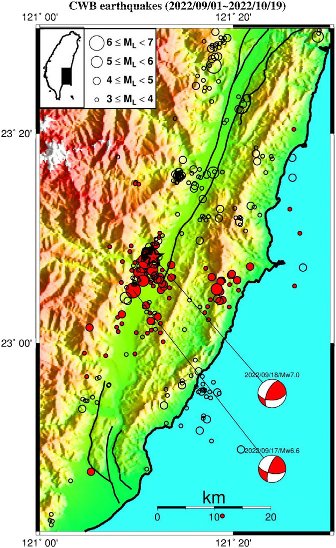
FIGURE 1. Epicenters of earthquakes (M_L≥3) from September to October 2022. Different sizes of red circles show the magnitudes of foreshocks. The mainshock is denoted by a large red solid star. Different sizes of open circles show the magnitudes of aftershocks. The thick solid lines mark the active faults. The index map in the upper left corner shows the study area (solid rectangle) and the different sizes of magnitude. The focal mechanisms of the foreshock and the mainshock are also plotted.

An earthquake (denoted by a large red solid star in Figure 1) with M_L=6.8 (M_L=the local magnitude determined by the Central Weather Administration, Taiwan) or M_w=7.0 (M_w=the moment magnitude determined by United States Geological Survey) occurred at Chihshang in the northern part of Taitung, eastern Taiwan, on 18 September 2022. Its epicenter inferred from the Central Weather Administration Seismological Network (CWASN) is located at 23.137^o N and 121.196^o E with a focal depth of 7.8 km. Before the mainshock, there were foreshocks with the largest one with M_L=6.6 or M_w=6.6 (denoted by a large red solid circle in Figure 1) that occurred on 17 September 2022. Its epicenter is located at 23.084^o N and 121.161^o E with a focal depth of 8.6 km. After the mainshock, many aftershocks happen. The largest aftershock with M_L=6.0 or M_w=5.6 occurred on 19 September 2022, about 20 h after the mainshock. Its epicenter is located at 23.441^o N and 121.300^o E with a focal depth of 13.4 km. The epicentral distribution of the earthquake sequence is displayed in Figure 1. The focal mechanisms of the foreshock and the mainshock are also plotted (IESRMT, 2022; Lee et al., 2023). Since such a kind of earthquake sequence does not occur frequently in the area, it is of great significance to study the spatial distribution and temporal variation of foreshocks and aftershocks.

Numerous studies focused on the correlation between foreshocks and mainshocks (e.g., Lin, 2009; De Santis et al., 2015; Gulia and Wiemer, 2019; Cianchini et al., 2020; Chen et al., 2023). Gulia and Wiemer (2019) studied the possible real-time discrimination between foreshock and aftershock sequences. De Santis et al. (2015) and Cianchini et al. (2020) applied the revised accelerated moment release to study the seismicity preceding large mainshocks. Chen et al. (2023) found that the bigger the largest foreshock is, the larger the mainshock is. Their research helps us understand the correlation between foreshocks and mainshocks.

Two important and basic scaling laws of seismicity are the frequency-magnitude (FM) relationship (Gutenberg and Richter, 1944) and the Omori law for aftershocks (Omori, 1894a, b; Utsu, 1957). The FM relationship represents the relation between the occurrence frequencies and magnitudes of earthquakes in an area. Omori (1894a, b) first proposed the Omori law to describe the number of aftershocks decreasing over time. Utsu (1961) modified Omori law as explained below.

In this study, we will explore the spatial and temporal distributions of events, temporal variations in the daily number of shocks, the distributions in the number of earthquakes in a unit of magnitude, and the temporal variations in seismic-wave energy for foreshocks and aftershocks. We will also study the frequency-magnitude relationships specified by the b-values for foreshocks, aftershocks, and the whole earthquake sequence, and aftershock decay with time characterized by the p-value.

2 The seismic-wave energy, FM relationship, and Omori-Utsu law

2.1 Seismic-wave energy

Gutenberg and Richter (1942; 1956) proposed the energy-magnitude law of earthquakes as follows:

$\log \left(E_s\right)=11.8+1.5M_s(1)$

in which E_s is the seismic-wave energy (in ergs) and M_s represents the surface-wave magnitude. Of course, M_s can be instead of the currently-used moment magnitude M_w. In Gutenberg and Richter (1942), Eq. 1 was inferred from the earthquakes with M_s≥5.5. From the evaluated values of E_s for small earthquakes from observed data, Wang (2015), Wang (2016a) confirmed that this equation can work for earthquakes with M_s<5.5.

Since we use the local magnitude in this study, M_s must be transferred to M_L in Eq. 1. Chen et al. (2007) derived the following M_L–M_s relationship for Taiwan earthquakes: M_s=−(0.53 ± 0.36)+ (1.03 ± 0.06)M_L. Substituting this relationship into Eq. 1 leads to

$\log \left(E_s\right)=11.01+0.76M_L(2)$

This study uses this formula to evaluate the values of E_s of events for the present earthquake sequence.

2.2 Gutenberg and Richter’s frequency-magnitude relationship

Gutenberg and Richter (1944) proposed a frequency-magnitude (FM) relationship for earthquakes in the form:

$\log \left(N\right)=a-bM(3)$

where M is the earthquake magnitude, N is the cumulative number of earthquakes with magnitudes ≥M, and a and b are constants. An example of the FM distribution based on the cumulative number of events is displayed in Figure 2. The FM relationship is only valid over the magnitude range between M₁ and M₂, which are, respectively, the lower and upper limits of the linear portion of the data points. Since we only attempt to compare the b-values between foreshocks and aftershocks, the values of M₁ and M₂ are estimated directly from the plots of log(N) versus M. We evaluated the value of M₁ just based on the observation that the data point started to bend down. The data points of M<M₁ will depart from the linear trend of data points with M≥M₁. The departure increases with decreasing M. We evaluated the value of M₂ just based on the observation that the data point started to depart from the linear trend of data points with M₁≤M≤M₂. Hence, they are estimated directly from the pattern of data points. The b-value will be estimated from the data points between M₁ and M₂ in two ways. The first one is the convenient linear squares method. The second way is based on the maximum likelihood method (e.g., Aki, 1965; Shi and Bolt, 1982). We will also compare the results estimated by the two methods.

FIGURE 2

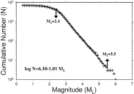
FIGURE 2. An example of the log(N) plots versus M_L for earthquakes.

The b-value varies by region and also depends on the time interval of the earthquake data used. The b-value is a scaling parameter related to the physical and geological conditions of the seismically active region (e.g., Scholz, 1968; Scholz, 2015; Wang, 1988; Wang, 2016b; Frohlich and Davis, 1993; Wiemer et al., 1998; Wang et al., 2015; Rivière et al., 2018).

2.3 Omori-Utsu law

Aftershocks are smaller events that follow the mainshock in and around the epicentral area. In addition to earthquake swarms, aftershocks are usually associated with most of moderate and large earthquakes. The earthquake magnitudes and the number of events usually decrease with time. Omori (1894a, b) first observed a decrease in the number of aftershocks as the time goes and proposed a power-law function to describe the change of the number of aftershocks, n(t), with time, t, in the following form: n(t)=k/(t+c), where k and c are two constants. This power law with scaling exponent 1 is called the Omori law and is the first scaling law in both seismology and the earth sciences. Utsu (1957) observed from experimental results that the number of aftershocks decays with Omori’s power law in the early stage, but exponentially in the late stage (e.g., Utsu, 1961; Mogi, 1962). Therefore, Utsu (1961) modified the Omori law as follows:

$n\left(t\right)=k/{\left(t+c\right)}^{\mathrm{p}},(4)$

where p is the scaling exponent of the power-law function that modifies the decay rate, typically in the range of 0.3–2.0 and usually close to 1. Utsu et al. (1995) explained in detail the physical meanings of k, c, and p. Equation 4 is commonly called the Omori-Utsu law or the modified Omori law. Because some larger aftershocks also produce their own aftershocks, the aftershock sequences are often very complicated, especially for large mainshocks. Therefore, it is also recommended to use other functions to describe the aftershock sequence (cf. Utsu et al., 1995; Shcherbakov et al., 2005; Iwata, 2016).

In the practical application, we may consider the cumulative number of aftershocks, N(t)=∫n(τ)dτ by integrating Eq. 4 from 0 to t (Utsu, 1961). The resulting equation is

$N\left(t\right)=k\left[c^{1-p}-{\left(c+t\right)}^{1-p}\right]/\left(p-1\right).(5)$

for p≠1 and

$N\left(t\right)=k\log \left(t/c+1\right).(6)$

for p=1. We will evaluate the values of k, c, and p from observed data based on Eq. 5 because of p≠1 after statistical tests.

3 Data

The Central Weather Administration (CWA), which was the Central Weather Bureau (CWB) before 15 September 2023, is responsible for the maintenance, operation, and observation of the Central Weather Administration Seismological Network (CWASN) in Taiwan. In addition to announcing real-time information on felt earthquakes in Taiwan, the network also provides the seismological community with information on every earthquake that occurs in Taiwan and high-quality digital seismic data. The uncertainty of the epicenter location is about ±2 km, and the uncertainty of the focal depth is about ±5 km (Shin and Chang, 2005). Earthquake magnitudes in earthquake catalogs have been unified into local earthquake magnitudes (Shin, 1992), denoted as M_L. Detailed descriptions of CWASN can be found in Shin (1992) and Shin and Chang (2005). The CWA has established an online data service platform at https://gdms.cwa.gov.tw. The data used in this study were retrieved directly from the CWA database at the website mentioned above. The earthquakes with M_L≥3 happened in the area from 22.7^o N to 23.5^o N and from 121.0^o E to 121.5^o E during the period from September to October 2022 were selected to study the characteristics of foreshocks and aftershocks of the 2022 Chihshang earthquake sequence. In the following, the focal depth of an event is denoted by ‘d’.

4 Results

4.1 Spatial and temporal distributions of earthquakes

The epicenters of the earthquake sequence with M_L≥3 are plotted in Figure 1 where the foreshocks, mainshock, and aftershocks are shown by solid circles, a star, and open circles, respectively. This figure exhibits that most of the events are located in the area around the Longitudinal Valley: some at the eastern side of the Central Range, some at the Coastal Range, and a few offshore. Figure 3 shows the time sequences of M_L≥3 earthquakes that occurred from September 1 to 19 October 2022: (a) for d≤25 km and (b) for d>25 km. This figure also shows that most of the events occurred in the depth range of 0–25 km and a few did below 25 km. Wang et al. (1994) reported that inland earthquakes in Taiwan mainly occur within the depth range of 0–12 km, and the number of earthquakes decreases significantly as the depth increases. Several authors (e.g., Rau and Wu, 1995; Ma et al., 1996; Kim et al., 2005) inferred the three-dimensional tomography in Taiwan. Their results show that the P-wave velocity at the crust-upper mantle boundary, mainly in the range of 35–45 km, is about 7.5 km. Therefore, the average depth of 40 km is used as the boundary to classify events: d≤40 km for a crustal event and d>40 km for an upper mantle or subduction zone event. Obviously, most events in the current earthquake sequence are crustal earthquakes as proven by Figure 3.

FIGURE 3

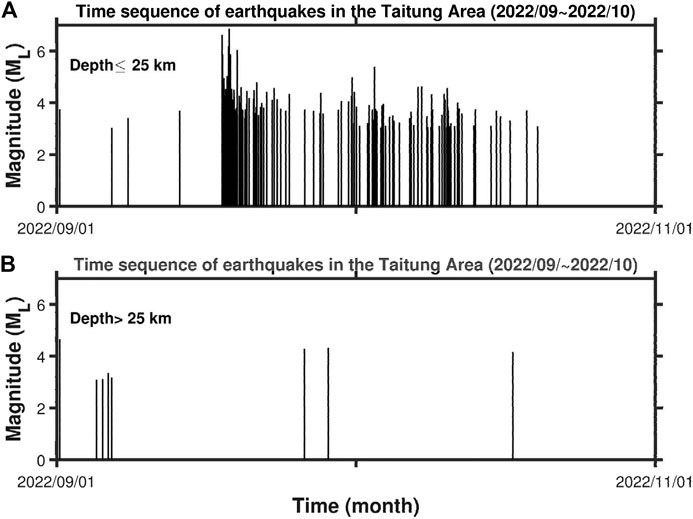
FIGURE 3. Time sequences of M_L≥3 earthquakes in the Taitung area: (A) for d≤25 km and (B) for d>25 km.

Figure 4 shows the time sequences of M_L≥3 earthquakes: (a) for the daily number of events and (b) for the cumulative number of events. The vertical dashed line denotes the occurrence time of the mainshock. From the two figures, we can see that only a few foreshocks occurred before September 17. A large number of events happened from the occurrence time of the largest foreshock to the largest aftershock and then the number of aftershocks decayed with time. Figure 4B shows a small cumulative number of events before the largest foreshock. The cumulative number of events increased rapidly from the occurrence time of the largest foreshock to that of the mainshock. The cumulative number of events increased almost linearly with time, with a moderately increasing rate in the first several days after the mainshock, and then the increasing rate gradually decreased with time.

FIGURE 4

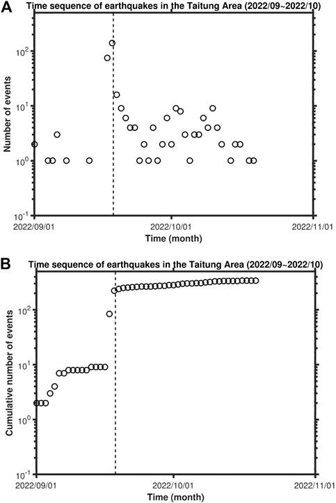
FIGURE 4. Time sequences of M_L≥3 earthquakes: (A) for the daily number of events and (B) for the cumulative number of events. The vertical dashed line denotes the occurrence time of the mainshock.

4.2 Temporal variation in seismic-wave energy

Figure 5 shows the temporal variation in seismic-wave energy, E_s, calculated from Eq. 2: (a) for the daily value of a sum of E_s’s of events occurring in 1 day and (b) for the cumulative value. The values of the largest foreshock and the mainshock are much higher than those of others. Hence, seismic-wave energies of the present earthquake sequence were mainly released by the largest foreshock and the mainshock.

FIGURE 5

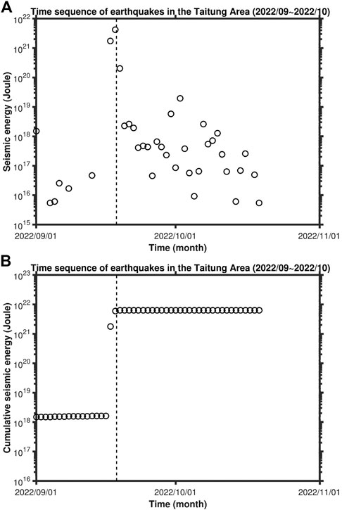
FIGURE 5. Time sequences of seismic-wave energy of M_L≥3 earthquakes: (A) for daily seismic energy and (B) for cumulative seismic energy. The vertical dashed line denotes the occurrence time of the mainshock.

4.3 Frequency-magnitude relationships

Figure 6 shows the numbers of M_L≥3 events in a unit of M_L: (a) for foreshocks; (b) for aftershocks; and (c) for the whole earthquake sequence. There are two local peaks with a large number of events for the three cases: 17 events at M_L=3.5 and 10 events at M_L=3.9 for foreshocks, 26 events at M_L=3.7 and 25 events at M_L=3.8 for aftershocks, and 35 events at M_L=3.7 and 33 events at M_L=3.8 for the whole earthquake sequence. Totally, most of the events appear in the magnitude range from 3.4 to 3.8 and the number of events at M_L=3.0 is also high.

FIGURE 6

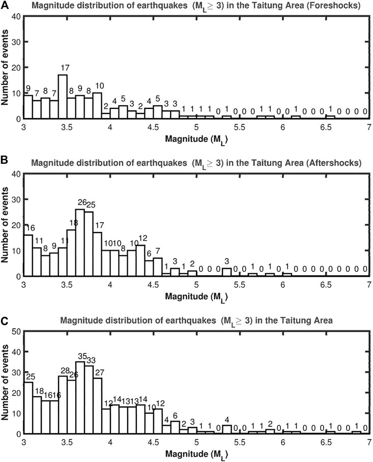
FIGURE 6. Numbers of M_L≥3 earthquakes versus M_L: (A) for foreshocks; (B) for aftershocks; and (C) for the whole earthquake sequence.

Figure 7, Figure 8, and Figure 9 demonstrate the plots of the cumulative number of events versus magnitude for foreshocks, aftershocks, and the whole earthquake sequence, respectively. The three figures reveal that the number of events obviously decreases as M_L<M₁. The values of M₁ are 3.0, 3.5, and 3.3, respectively, for the three figures. This is the reason why only the events with M_L≥3.0 are shown in this study. The data points for the three figures are almost around a line. The values of M₂ are 6.7, 6.0, and 6.8 for Figure 7, Figure 8 and Figure 9, respectively. Since the mainshock with M_L=6.8 is not taken for the regression of the FM relationships for Figure 7 and Figure 8, we may evaluate the FM relationships only for foreshocks and aftershocks, respectively. The inferred FM relationships by using the least squares method are structured

$\log \left(N\right)=\left(4.05\pm 0.05\right)-\left(0.62\pm 0.01\right)M_L(7)$

for foreshocks (M₁=3.0≤M_L≤M₂=6.6);

$\log \left(N\right)=\left(5.30\pm 0.12\right)-\left(0.87\pm 0.03\right)M_L(8)$

for aftershocks (M₁=3.5≤M_L≤M₂=6.0); and

$\log \left(N\right)=\left(4.85\pm 0.07\right)-\left(0.71\pm 0.01\right)M_L(9)$

for the whole earthquake sequence (M₁=3.3≤M_L≤M₂=6.8). Eqs. 7 and (8), and (9) are represented by a solid line in Figure 7, Figure 8 and Figure 9, respectively.

FIGURE 7

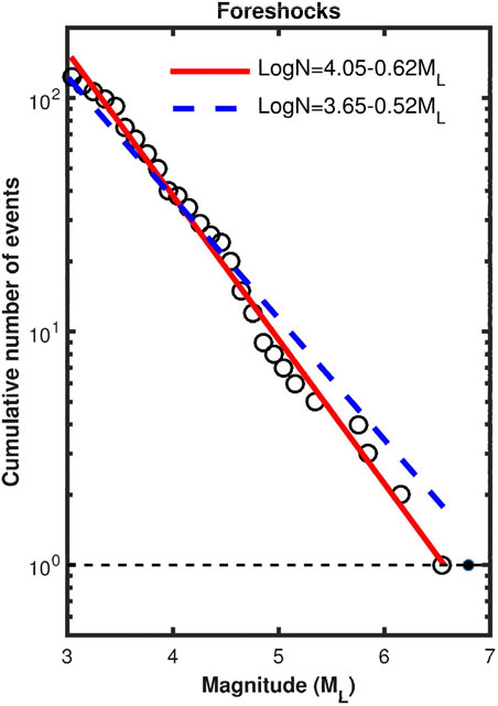
FIGURE 7. The plot of log(N) (N=cumulative number of foreshocks, open circle) versus M_L. The solid circle denotes the mainshock with magnitude M_L6.8. The dashed line denotes log(N)=0 because of N=1. The thick red solid line and thick blue dashed line represent the estimation of b value through least squares and maximum likelihood techniques, respectively.

FIGURE 8

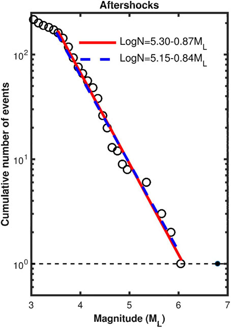
FIGURE 8. The plot of log(N) (N=cumulative number of aftershocks, open circle) versus M_L. The solid circle denotes the mainshock with magnitude M_L6.8. The dashed line denotes log(N)=0 because of N=1. The thick red solid line and thick blue dashed line represent the estimation of b value through least squares and maximum likelihood techniques, respectively.

FIGURE 9

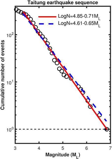
FIGURE 9. The plot of log(N) (N=cumulative number of events, open circle) versus M_L. The solid circle denotes the mainshock with magnitude M_L6.8. The dashed line stands log(N)=0 because of N=1. The thick red solid line and thick blue dashed line represent the estimation of b value through least squares and maximum likelihood techniques, respectively.

The inferred FM relationships by using the maximum likelihood method are

$\log \left(N\right)=\left(3.65-0.52M_L\right)\pm 0.04(10)$

for foreshocks (M₁=3.0≤M_L≤M₂=6.6);

$\log \left(N\right)=\left(5.15-0.84M_L\right)\pm 0.06(11)$

for aftershocks (M₁=3.5≤M_L≤M₂=6.0); and

$\log \left(N\right)=\left(4.61-0.65M_L\right)\pm 0.03(12)$

for the whole earthquake sequence (M₁=3.3≤M_L≤M₂=6.8). Eqs. 10 and (11), and (12) are represented by a dashed line in Figure 7, Figure 8 and Figure 9, respectively. The b-values are smaller from the maximum likelihood estimates than from the least squares estimates and the difference is the smallest for aftershocks and the largest for foreshocks. For foreshocks, it seems that the solid line from the least squares method fits the data points better than the dashed line from the maximum likelihood method.

4.4 Omori-Utsu law

The ZMAP software (Wiemer, 2001) was used to estimate the parameters of the Omori-Utsu law. Figure 10A presents a plot of the cumulative number of aftershocks as a function of time, shown by the solid line. In comparison with the first 3 days, the increasing rate of the cumulative number of aftershocks remarkably decreased from the third day to the 22nd day. Nevertheless, we still inferred the Omori-Utsu law for the aftershocks. Based on Eq. 5, the inferred law from the data (with c=0.02 days) is

$n\left(t\right)=27.7/{\left(t+0.02\right)}^{0.92}.(13)$

FIGURE 10

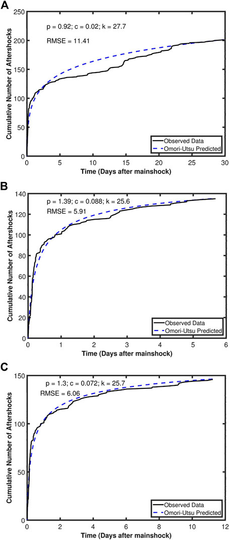
FIGURE 10. Time variation in the cumulative number of M_L≥3 aftershocks as a function of time, (A) for 30 days, (B) for 6 days, and (C) for 12 days after the mainshock. The solid line denotes observed data and the dashed line represents the inferred Omori-Utsu law. The inferred parameters p, c, k and the root mean square error (RMSE) are also shown in the upper left corner of the figure.

The inferred law is shown as the dashed line in Figure 10A. The estimated parameters p, c, k and the root mean square error (RMSE) are also shown in the upper left corner of the figure. The dashed line fits very well with the solid line in the first 3 days and last few days; while it departs from the solid line from the third day to the 22nd day. The data of aftershocks suffer from short-term incompleteness as shown in Figure 10A. This effect could produce a bias in the calculation of the p-value. Hence, we plotted two more figures, i.e., Figure 10B and Figure 10C, displaying the time variation in the cumulative number of aftershocks from 0 to about the sixth day and from 0 to about the 12th day, respectively. The estimated p-value is 1.39 for the former and 1.30 for the latter. As mentioned above, the p-value is 0.92 for the whole period in consideration. Results show a decrease in p-values with increasing time. This implicates a decrease in the decay rate of aftershocks with increasing time.

5 Discussion

5.1 Spatial and temporal distributions of earthquakes

Figure 1 displays the epicentral distribution of 341 M_L≥3 events of the earthquake sequence. It seems that the events may be divided into two groups: the foreshocks (shown with red circles) occurred from September 17 to September 18 and the aftershocks (displayed with open circles) happened from September 18 to October 19. The foreshocks occurred in the area from 23^o55′ N to 23^o15′ N and from 121^o08′ E to 121^o25′ E; while the aftershocks happened in the area from 22^o52′ N to 23^o30′ N and from 121^o05′ E to 121^o20’ E. The area of foreshocks is smaller than that of aftershocks. There was an overlap of the two areas, and aftershocks expanded outwards from the foreshock area. The migration of seismicity from the foreshock zone to the aftershock zone reflects the time history of post-earthquake readjustment of the tectonic balance. Seismic migration can also be observed in the 1986 Hualien earthquake sequence (Chen and Wang, 1986; Chen and Wang, 1988) and the 2018 Hualien earthquake sequence (Kou-Chen et al., 2019).

Wang (2021) and Chen et al. (2023) addressed the positive correlation between the mainshock and its largest foreshock for earthquake sequences in Taiwan. From 38 earthquake sequences whose mainshocks with M_L were in the range from 4.6 to 6.8 during 1983–2022, Chen et al. (2023) inferred the relationship between the magnitude of the mainshock and that of the largest foreshock. Their result is M_L=(1.59 ± 0.47)+(0.79 ± 0.10)M_Lf, where M_Lf is the magnitude of the largest foreshock. Although there are numerous models concerning the generation and evolution of foreshocks (e.g., Yamashita and Knopoff, 1989; Sornette et al., 1992), there is a lack of theoretical study to correlate the largest foreshock and the mainshock. Hence, we can only try to apply the empirical relation between the magnitude of the largest foreshock and the mainshock magnitude inferred from 38 Taiwan earthquake sequences to estimate the mainshock magnitude from the magnitude of the largest foreshock. Actually, only a small percentage of mainshocks were proceeded by foreshocks for world-wide and Taiwan earthquakes. However, there were both foreshocks (including the largest foreshock) and the mainshock for the present earthquake sequence. This is an opportunity for us to test the above-mentioned relation and to explore the possibility of predicting the mainshock magnitude from the magnitude of the largest foreshock. Since M_Lf is 6.6 of the present earthquake sequence, the estimated value of M_L of the mainshock is 6.8 which is the same as the observed value of M_L=6.8. This confirms the feasibility of using this formula to predict the magnitude of the mainshock for some Taiwan earthquake sequences for which the foreshocks occurred.

Figure 3A shows the time sequence of earthquake magnitudes for 333 M_L≥3 events with d≤25 km. The time sequence of earthquakes is not uniform. The frequency of earthquakes is higher during some short time intervals and lower during other time intervals. The largest inter-event time is 5.208 days and the shortest one is smaller than 1 day.

Figure 3B shows that there are only eight events with d>25 km. This number of events is much smaller than the number of events with d≤25 km. This indicates that the earthquake sequence occurred mainly in the upper crust. The time interval between any two consecutive events with d>25 km is mostly longer than 1 day, thus indicating low dependence from one to the other.

Figure 4 shows the time sequences of M_L≥3 earthquakes: (a) for the daily number and (b) for the cumulative number of events. Clearly, there are only 9 events before the largest foreshock on 17 September 2022. As shown in Figure 4A and Figure 4B, 2 earthquakes occurred on September 2; 1 event happened on September 4 and 5; 3 earthquakes occurred on September 6; and 1 earthquake occurred on September 8 and 13. The foreshock activity was very low and uniform in a time interval of 16 days before the largest foreshock and then rapidly increased 1 day before the mainshock. Kagan and Knopoff (1978) and Jones and Molnar (1979) first observed that the number of foreshocks increases with time almost following a power-law function. The pattern of seismic activity of foreshocks in this study somehow shows an increase in the number of daily events over time (Figure 4A).

5.2 Time sequence of seismic-wave energy, E_s

Figure 5 shows the time sequences of E_s: (a) for the daily values and (b) for the cumulative values. Results reveal that most of the seismic-wave energy of the earthquake sequence was released by the largest foreshock and the mainshock, while the largest aftershock and other events only made a minor contribution. This is due to the fact that the magnitudes of foreshocks and aftershocks are much smaller than those of the largest foreshock and the mainshock. In addition, the temporal variation in E_s for foreshocks is similar to that of aftershocks, even though the numbers of events for them are quite different.

5.3 Frequency-magnitude relationships

Figure 6 shows the numbers of M_L≥3 events in a unit of M_L: (a) for foreshocks; (b) for aftershocks; and (c) for the whole earthquake sequence. Most of the events appear in the magnitude range from 3.4 to 3.8 and the number of events at M_L=3.0 is also high. The ratio of the number of larger events (M_L≥4) to that of smaller ones (M_L<4) is generally higher for aftershocks than for foreshocks.

From Figure 7 and Figure 8, the b-values are 0.62 and 0.87 from the least squares estimate and 0.52 and 0.84 from the maximum likelihood estimate, respectively, for foreshocks and aftershocks. The estimated b-values are larger from the least squares estimate than from the maximum likelihood estimate. The difference is larger for foreshocks than for aftershocks. Wang (1988) measured the b-values for shallow earthquakes in Taiwan. His b-values are taken as background ones for this study because Wang (1988) used earthquake data before 1988 which would be almost not related to recent seismicity. The b-values in the present study area are between 1.0 and 1.2 with an average of 1.1. In his study, an earthquake was quantified by the duration magnitude, M_D, and thus the FM relationship is log(N)=a’-b’M_D. We must transfer this b-value, i.e., b’, into the present one based on local magnitude, M_L. Wang et al. (1989) correlated M_D with M_L in the relation: M_D=(0.187 ± 0.373)+(0.862 ± 0.066)M_L. The FM relationship: log(N)=a’-b’M_D becomes log(N)=a’-b’(0.862M_L+0.187)=(a’-0.187b′)-0.862b′M_L. This makes the average b-value in terms of b’ in the study area to be 0.862b’. Hence, the average background b-value which is 0.862 × 1.1=0.95 (average b’=1.1) based on the local magnitude. This makes the b-values of the aforementioned foreshocks and aftershocks both lower than the background ones.

In addition, the b-value is smaller for foreshocks than for aftershocks, with a difference of 0.25 from the least squares method and 0.32 from the maximum likelihood method. From measured b-values for the earthquake sequences occurring in eight seismic regions around the world, Wetzler et al. (2023) found that the b-values of foreshocks are lower by 0.1–0.2 than those of respective aftershocks. In their study, the earthquake magnitude is M_w or M_s. In this study, we use the local magnitude, M_L. It is necessary to consider the effect on the estimates of b-values due to different magnitude scales. Chen et al. (2007) inferred the conversion relation between M_s and M_L, i.e., M_s=(1.03 ± 0.06)M_L-(0.53 ± 0.36). Hence, the FM relationship in M_s, i.e., log(N)=a^*-b^*M_s, becomes log(N)=a^*-b^*(1.03M_L-0.53)=(a^*+ 0.53b^*)-1.03b^*M_L. This relation gives b^*=0.60 for the foreshocks and 0.85 for the aftershocks, and thus the difference between the two values is 0.25, based on the least squares method. This relation gives b^*=0.50 for the foreshocks and 0.82 for the aftershocks, and thus the difference between the two values is 0.32, based on the least squares method. The present result is more consistent with that obtained by Wetzler et al. (2023) for the least squares method than for the maximum likelihood method.

From simulation results based on a one-dimensional spring-slider model (Burridge and Knopoff, 1967), Wang (1995) studied the correlation between b and s=K/L, where K and L are the spring constant between two sliders and that between a slider and the moving plate, respectively. His results yielded the power-law correlations between b and s: b∼s^-2/3 for the cumulative frequency and b∼s^-1/2 for the discrete frequency. Since L of an area is almost constant for a long time period, b is related to K. A smaller (larger) K results in a higher (lower) b-value. Hence, the K value for aftershocks is smaller than that for foreshocks. This means that the coupling between two faults or fault segments (represented by two sliders) changes from stronger for foreshocks to weaker for aftershocks. Wang (2012) obtained K=ρ_Av_p², where ρ_A and v_p are the areal density and P-wave velocity of the fault zone, respectively. This means that s is related to the P-wave velocity in the fault zone. Experimental results show that v_p is greatly affected by the water saturation in rocks (e.g., Cadoret et al., 1995). Wang (2016b) correlated s with the degree of saturation of fluids in a fault zone. The water saturation within the fault zone varies with time, causing v_p and K to change with time. The degree of water saturation almost reached 100% in a short time interval in the related fault zone before the occurrence of mainshock, thus yielding high pore pressure to reduce the normal stress on the main fault zone. This makes the main fault easily failure and then the mainshock happens. The degree of water saturation rapidly decreases after the mainshock. Aftershocks are introduced by stress transfer (e.g., Ma et al., 2005; Cattania et al., 2015) and migration of fluids (e.g., Yamashita and Knopoff, 1989; Yamashita, 1998; Yamashita, 2003) from the source area to the surrounding areas where the aftershocks are triggered. This suggests that the degree of water saturation in the sub-faults linking to the main fault was higher for the foreshocks and lower for the aftershocks due to outward water migration from the epicentral and foreshock areas to a wider surrounding areas. This produces a change from a higher s value to a lower one, thus resulting in a temporal change in the b-values from a smaller value to a larger one in the area around the source area before and after the mainshock.

An interesting question arises whether the magnitudes of the mainshock, the largest foreshock, and the largest aftershock of the 2022 Chihshang earthquake sequence can be estimated based on their respective FM relationships log(N)=a–bM_L just by letting log(N)=0 because of N=1, thus leading to M_L=a/b? The estimated value of M_L of the largest foreshock is ∼6.5 from Eq. 7. The value is 0.1 smaller than the magnitude for the largest foreshock, i.e., M_L=6.6. In addition, the estimated value of M_L of the largest aftershock is ∼6.1 from Eq. 8. The value is 0.1 larger than the magnitude for the largest aftershock, i.e., M_L=6.0. The estimated value of M_L of the mainshock is ∼6.8 from Eq. 9. The value is the same magnitude for the mainshock, i.e., M_L=6.8. Results seem to suggest that our answer to the question is positive for the present earthquake sequence. Of course, we cannot answer the question whether the present results can be applied to other earthquake sequences.

For aftershocks, Båth’s law (Båth, 1965; Båth, 1984) states that the difference between the magnitude of the mainshock and that of the largest aftershock is on average a constant, typically to be 1.2 for macroseismic magnitude (Båth, 1965) and 1.4 for local magnitude (Båth, 1984). The magnitude of the largest aftershock of the present earthquake sequence is M_L=6.0. The difference between the magnitude of the mainshock and that of the largest aftershock is 0.8, which is 0.4 smaller than 1.2 from Båth’s law. Shcherbakov and Turcotte (2004) proposed the modified version of Båth’s law from the extrapolation of the FM relationship for aftershocks. They defined the magnitude of the largest aftershock as a/b. Hence, the difference between the magnitude of the mainshock and that of the largest aftershock is 0.7, which is 0.5 smaller than 1.2 from Båth’s law. Consequently, Båth’s law does not seem able to work for the present earthquake sequence. For Taiwan’s earthquakes, several authors (e.g., Wang and Wang, 1993; Chen and Wang, 2012; Wang, 2016b) reported the difference between the magnitude of the mainshock and that of its largest aftershock increases with the former. Their results are also different from Båth’s law.

Figure 9 with Eq. 9 shows b=0.71 for the whole earthquake sequence. This b-value is just between that for foreshocks and that for aftershocks. The intersection point of the line of the FM relationship at the horizontal dotted line with log(N)=0 is at M_L=6.8 which is exactly the mainshock magnitude. This suggests that the FM distribution of the earthquake sequence is complete, at least, for M_L≥3 events.

5.4 Omori-Utsu law

Figure 10A shows that in comparison with the first 3 days, the increasing rate of the cumulative number of aftershocks remarkably decreased from the third day to the 22nd day. This indicates a decrease in M_L≥3 earthquakes in this time period. This kind of phenomenon has also been observed by other authors (e.g., Båth, 1984; Matsu’ura 1986). Matsu’ura (1986) addressed that such a phenomenon is due to the inhomogeneity of data in use. From Figure 10A with Eq. 13, the p-value is 0.92 for aftershocks. This value is in the range of observed results for world-wide earthquakes (e.g., Utsu, 1961; Wang, 1994).

The data of aftershocks suffer from short-term incompleteness, especially in the time period of the fifth day to the twenty-first day after the mainshock, as shown in Figure 10A. Figure 3 also displays a decrease in aftershocks in this time period. This effect could produce a bias in the calculation of the p-value. Hence, we added two new figures, i.e., Figure 10B and Figure 10C, displaying the time variation in the cumulative number of aftershocks from 0 to about the sixth day and from 0 to about the 12th day, respectively. The estimated p-value is 1.39 for the former and 1.30 for the latter. As mentioned above, the p-value is 0.92 for the whole period in consideration. Results show a decrease in p-values with increasing time. This implicates a decrease in the decay rate of numbers of aftershocks with increasing time.

Several authors (e.g., Kagan and Knopoff, 1978; Yamashita and Knopoff, 1989; Sornette et al., 1992) proposed the inverse Omori law: n(t)=κ/(t_f-t)^p, where t_f is the failure time of the mainshock. In their model, the peak number appears just before the mainshock. As shown in Figure 4, a total of only 9 events occurred in the 16 days before the largest foreshock in the study area. Foreshock activity mainly occurred 18 h before the mainshock. Figure 11 shows the temporal variation of the number of foreshocks in each hour before the mainshock. Such a time variation cannot be described by the inverse Omori law.

FIGURE 11

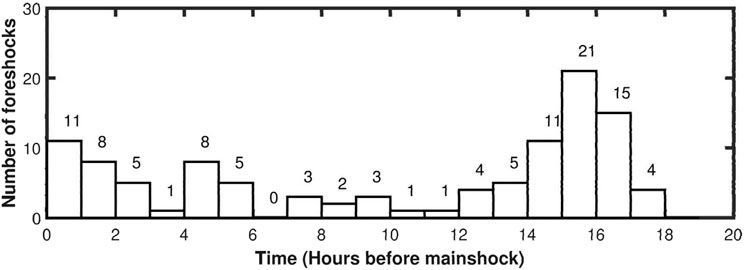
FIGURE 11. Temporal changes in the number of M_L≥3 foreshocks per hour in the 18 h before the mainshock.

It is interesting to study the correlation between the p-value and the b-value. Utsu (1961) first stated that, for the Japanese earthquake, the p-values are related to the b values ranging from 0.3 to 2.0 in the form of p=4b/3. Since then, numerous authors (Yamashita and Knopoff, 1989; Guo and Ogata, 1995; 1997; Utsu et al., 1995; Helmstetter and Sornette, 2002; Zaccagnino et al., 2022) theoretically studied the correlation between the two parameters. Zaccagnino et al. (2022) proposed p=2(1+b)/3 based on physical mechanism. Guo and Ogata (1997) and Helmstetter and Sornette (2002) used the b and p values of the early aftershock sequences to conduct aftershock prediction based on the Epidemic-Type Aftershock Sequence (ETAS) model (Ogata, 1986). In addition, some authors (e.g., Ma et al., 1990; Wang, 1994) observed a negative correlation between b and p for these two parameters from earthquake data. Since Ma et al. (1990) and Wang (1994) did not construct the relationship between the two parameters, we here only consider the positively correlated relationship. The evaluated p-value is 1.16 from p=4b/3 (Utsu, 1961) and 1.25 from p=2(1+b)/3 by Zaccagnino et al. (2022) because of b=0.87 from Eq. 8. In comparison with the p-value in Eq. 13, the p-values estimated from the relationships done by Utsu (1961) and Zaccagnino et al. (2022), respectively, are higher than the p-value (=0.92) for the present observation for the whole period in consideration and smaller than that (=1.39) from 0 to about the sixth day as well as that (=1.3) from 0 to about the 12th day. This suggests the importance of time interval of aftershocks for the estimate of p-value.

In addition to the Omori-Utsu law, there are numerous laws that have been used to describe the aftershock decay (cf. Mignan, 2015). For example, Souriau et al. (1982) proposed the stretched exponential function, i.e., n(t)=αβt^(β−1)exp(-αt^β) where α and β are two parameters, to describe the aftershock decay. This function is different from the Omori-Utsu law. Based on the maximum likelihood method, Kisslinger (1993) estimated the parameters in the stretched exponential function for the aftershock decay of 29 earthquake sequences. He found that if the occurrence time of the mainshock is taken as the start time, the Omori-Utsu law is almost always better. On the other hand, if a later start time is used, 15 min to 2.5 h for his cases tested, the stretched exponential function is better. For the present earthquake sequence, the Omori-Utsu law is acceptable because the start time is just the occurrence time of the mainshock. Mignan (2015) compared the power-law function, pure exponential function, i.e., n(t)=c exp(-αt) where c and α are two parameters (Burridge and Knopoff, 1967), and stretched exponential function to describe the aftershock decay in a long time (from 10⁻⁴ days to almost 10⁴ days) for earthquake sequences in three regions, i.e., Southern California, Northern California, and Taiwan. He applied three statistical methods for declustering, i.e., the nearest-neighbor, second-order moment, and window methods. His results suggest that aftershock decay follows a stretched exponential instead of a power law. Hence, he inferred that aftershocks are due to a simple relaxation process, following most other relaxation processes observed in Nature. Our results show that the Omori-Utsu law works well for the aftershock decay in the first 12 days after the mainshock. This is different from Mignan’s assumption. Of course, the aftershock decay after the 12th day departed remarkably from the Omori-Utsu law. After examining the results shown in Figure 2 of Mignan (2015), it is difficult to say whether the stretched exponential function may be applied to the present results or not.

Numerous authors (e.g., Ouillon and Sornette, 2005; Ouillon et al., 2009) assumed that the Omori law is magnitude-dependent. This means that the p-value depends on the magnitude of the mainshock. For Taiwan’s earthquakes, Tsai et al. (2012) inferred the following relationship between p and M_w: p(M_w)≃(0.38 ± 0.02)+(0.11 ± 0.01)M_w (2.6≤M_w≤7.6), where M_w is the moment magnitude of the mainshock. From this equation, the estimated p(M_w) values are in the range of 1.06–1.24 with a median value of 1.15 due to M_w=7.0 of the mainshock. The observed p-value of the aftershocks occurred in 30 days after the mainshock is 0.92 which is outside the range of estimated values and 0.23 lower than the median one. The observed p-value of the aftershocks occurred in 6 days after the mainshock is 1.39 which is outside the range of estimated values and 0.24 higher than the median one. The observed p-value of the aftershocks occurred in 12 days after the mainshock is 1.30 which is slightly outside the range of estimated values and 0.15 higher than the median one. The three observed p-values are different from the p-value estimated from the p-M_w equation.

From numerous earthquake sequences in Taiwan, Chen and Wang (2012) did not find any positive correlation between the mainshock and the largest aftershock. Hence, we do not consider the possible correlation between them for the present earthquake sequence.

6 Conclusion

An earthquake with M_L6.8 occurred at 23.137^o N and 121.196^o E with a focal depth of 7.8 km at Chihshang in the northern part of Taitung, eastern Taiwan on 18 September 2022. We analyzed seismicity with M_L≥3 and d≤25 km, that occurred before and after, respectively, the mainshock, to explore the epicentral distributions and temporal variations of the foreshocks and aftershocks. Results exhibit that most of the events are located in the area around the Longitudinal Valley: some at the eastern side of the Central Range, some at the Coastal Range, and a few offshore. The foreshocks occurred in a smaller area around the mainshock epicenter and the aftershocks happened outwards from the mainshock epicenter. The temporal variations in seismic-wave energy of the earthquake sequence are taken into account. In addition, the frequencies of events counted in a unit of magnitude, and the b-values of Gutenberg-Richter frequency-magnitude relationships for foreshocks, aftershocks, and the whole earthquake sequence are evaluated. The b-values are different for foreshocks, aftershocks, and the whole earthquake sequence. The p-value of Omori-Utsu law for aftershocks is also estimated. The seismic-wave energies of the earthquake sequence were mainly released by the largest foreshock and the mainshock. The b values are 0.62 for foreshocks, 0.87 for aftershocks, and 0.71 for the whole earthquake sequence. The b values increase from foreshocks to aftershocks, suggesting a possibility that the fluid pressure in the fault zone is higher before the mainshock, and that pore pressure of the faults is lower during the seismic sequence. The estimated p-values are 0.92 for all aftershocks in the study, 1.39 for the aftershocks occurred in the first 6 days, and 1.30 for the aftershocks occurred in the first 12 days. The p-values seem to decrease with increasing time interval is a mirror of progressive stabilization of seismic activity over time. The p-values estimated at different time intervals would have different correlations with the b-values of aftershocks. At last, we notice that foreshocks are not described by the inverse Omori law.

Data availability statement

The original contributions presented in the study are included in the article/Supplementary material, further inquiries can be directed to the corresponding author.

Author contributions

K-CC: Conceptualization, Investigation, Writing–original draft, Writing–review and editing. B-SH: Project administration, Writing–review and editing. K-HK: Writing–review and editing. J-HW: Writing–review and editing.

Funding

The author(s) declare financial support was received for the research, authorship, and/or publication of this article. This study was supported by Academia Sinica, under grant AS-TP-110-M02 (B-SH), the Central Weather Bureau, under grant MOTC-CWB-112-E−02 (B-SH), the National Science and Technology Council, Taiwan, under grant NSTC 111-2116-M-001-011 (B-SH), and partially by the Korean Meteorological Administration Research Development Program, under grant KMI 2022-00610 (K-HK).

Acknowledgments

We would like to express our deep thanks to three reviewers and Editor of the Journal, Prof. Di Giovambattista, for their valuable comments and suggestions, which helped us to significantly improve this article. The authors also wish to express their appreciation to the Central Weather Administration, Taiwan for providing data used in this study.

Conflict of interest

The authors declare that the research was conducted in the absence of any commercial or financial relationships that could be construed as a potential conflict of interest.

Publisher’s note

All claims expressed in this article are solely those of the authors and do not necessarily represent those of their affiliated organizations, or those of the publisher, the editors and the reviewers. Any product that may be evaluated in this article, or claim that may be made by its manufacturer, is not guaranteed or endorsed by the publisher.

References

Aki, K. (1965). Maximum likelihood estimate of b in the formula logN=a-bM and its confidence limits. Bull. Earthq. Res. Inst. Tokyo Univ. 43, 237–239.

Google Scholar

Båth, M. (1965). Lateral inhomogeneities of the upper mantle. Tectonophys 2, 483–514. doi:10.1016/0040-1951(65)90003-x

CrossRef Full Text | Google Scholar

Båth, M. (1984). A note on Fennoscandian aftershocks. Bull. Geopfis. Teor. Appl. XXVI (104), 211–220.

Google Scholar

Burridge, R., and Knopoff, L. (1967). Model and theoretical seismicity. Bull. Seism. Soc. Am. 57, 341–371. doi:10.1785/bssa0570030341

CrossRef Full Text | Google Scholar

Cadoret, T., Marion, D., and Zinszner, B. (1995). Influence of frequency and fluid distribution on elastic wave velocities in partially saturated limestones. J. Geophys. Res. 100, 9789–9803. B6. doi:10.1029/95jb00757

CrossRef Full Text | Google Scholar

Cattania, C., Hainzl, S., Wang, L., Enescu, B., and Roth, F. (2015). Aftershock triggering by postseismic stresses: a study based on Coulomb rate-and-state models. J. Geophys. Res. Solid Earth 120, 2388–2407. doi:10.1002/2014JB011500

CrossRef Full Text | Google Scholar

Chen, H. Y., Kuo, L. C., and Yu, S. B. (2004). Coseismic movement and seismic ground motion associated with the 31 March 2002 off Hualien, Taiwan, earthquake. Terr. Atmos. Ocean. Sci. 15 (4), 683–695. doi:10.3319/tao.2004.15.4.683(t)

CrossRef Full Text | Google Scholar

Chen, K. C. (2003). Strong ground motion and damage in the Taipei basin from the Moho reflected seismic waves during the March 31, 2002, Hualien, Taiwan earthquake. Geophys. Res. Lett. 30. doi:10.1029/2003GL017193

CrossRef Full Text | Google Scholar

Chen, K. C., Huang, W. G., and Wang, J. H. (2007). Relationships among magnitudes and seismic moment of earthquakes in the Taiwan region. Terr. Atmos. Ocean. Sci. 18 (5), 951–973. doi:10.3319/tao.2007.18.5.951(t)

CrossRef Full Text | Google Scholar

Chen, K. C., Kim, K. H., and Wang, J. H. (2023). On the correlations between the largest foreshocks and mainshocks of earthquake sequences in Taiwan. Front. Earth Sci. 11, 1233487. doi:10.3389/feart.2023.1233487

CrossRef Full Text | Google Scholar

Chen, K. C., Kim, K. H., Wang, J. H., and Chen, K. C. (2022). Dominant periods and memory effect of the 2021 earthquake swarm in Hualien, Taiwan. Terr. Atmos. Ocean. Sci. 33, 24. doi:10.1007/s44195-022-00022-2

CrossRef Full Text | Google Scholar

Chen, K. C., and Wang, J. H. (1986). The may 20, 1986 haulien, taiwan earthquake and its aftershocks. Bull. Inst. Earth. Sci. Acad. Sin. 6, 1–13.

Google Scholar

Chen, K. C., and Wang, J. H. (1988). A study on aftershocks and focal mechanisms of two 1986 earthquakes in Hualien, Taiwan. Proc. Geol. Soc. China 31, 65–72.

Google Scholar

Chen, K. C., and Wang, J. H. (2012). Correlations between the mainshock and the largest aftershock for taiwan earthquakes. Pure Appl. Geophys. 169, 1217–1229. doi:10.1007/s00024-011-0352-9

CrossRef Full Text | Google Scholar

Chen, K. H., Toda, S., and Rau, R. J. (2008). A leaping, triggered sequence along a segmented fault: the 1951 M_L7.3 Hualien-Taitung earthquake sequence in eastern Taiwan. J. Geophys. Res. 113, B02304. doi:10.1029/2007JB005048

CrossRef Full Text | Google Scholar

Cianchini, G., De Santis, A., Di Giovambattista, R., Abbattista, C., Amoruso, L., Campuzano, S. A., et al. (2020). Revised accelerated moment release under test: fourteen worldwide real case studies in 2014–2018 and simulations. Pure Appl. Geophys. 177, 4057–4087. doi:10.1007/s00024-020-02461-9

CrossRef Full Text | Google Scholar

De Santis, A., Cianchini, G., and Di Giovambattista, R. (2015). Accelerating moment release revisited: examples of application to Italian seismic sequences. Tectonophys 639, 82–98. doi:10.1016/j.tecto.2014.11.015

CrossRef Full Text | Google Scholar

Frohlich, C., and Davis, S. D. (1993). Teleseismic b values; or, much ado about 1.0. J. Geophys. Res. 98, 631–644. B1. doi:10.1029/92JB01891

CrossRef Full Text | Google Scholar

Gulia, L., and Wiemer, S. (2019). Real-time discrimination of earthquake foreshocks and aftershocks. Nature 574, 193–199. doi:10.1038/s41586-019-1606-4

PubMed Abstract | CrossRef Full Text | Google Scholar

Guo, Z., and Ogata, Y. (1995). Correlation between characteristic parameters of aftershock distributions in time, space and magnitude. Geophys. Res. Letts. 22 (8), 993–996. doi:10.1029/95gl00707

CrossRef Full Text | Google Scholar

Guo, Z., and Ogata, Y. (1997). Statistical relations between the parameters of aftershocks in time, space, and magnitude. J. Geophys. Res. Solid Earth 102, 2857–2873. B2. doi:10.1029/96jb02946

CrossRef Full Text | Google Scholar

Gutenberg, B., and Richter, C. F. (1942). Earthquake magnitude, intensity, energy and acceleration. Bull. Seism. Soc. Am. 32, 163–191. doi:10.1785/bssa0320030163

CrossRef Full Text | Google Scholar

Gutenberg, B., and Richter, C. F. (1944). Frequency of earthquakes in California. Bull. Seism. Soc. Am. 34, 185–188. doi:10.1785/bssa0340040185

CrossRef Full Text | Google Scholar

Gutenberg, B., and Richter, C. F. (1956). Magnitude and energy of earthquake. Ann. Geofis. 9, 1–15.

Google Scholar

Helmstetter, A., and Sornette, D. (2002). Subcritical and supercritical regimes in epidemic models of earthquake aftershocks. J. Geophys. Res. Solid Earth 107. (B10), ESE 10-1-ESE 10-21. doi:10.1029/2001jb001580

CrossRef Full Text | Google Scholar

Hsu, M. T. (1961). Seismicity of taiwan (formosa). Bull. Earthq. Res. Inst. Tokyo Univ. 39, 831–847.

Google Scholar

Hsu, M. T. (1971). Seismicity of Taiwan and some related problems. Bull. Int. Inst. Seism. Earthq. Engin. Jpn. 8, 41–160.

Google Scholar

Hwang, R. D., Huang, Y. L., Chang, W. Y., Lin, C. Y., Lin, C. Y., Wang, S. T., et al. (2022). Radiated seismic energy from the 2021 M_L5.8 and M_L6.2 Shoufeng (Hualien), Taiwan, earthquakes and their aftershocks. Terr. Atmos. Ocean. Sci. 33, 19. doi:10.1007/s44195-​022-​00020-4

CrossRef Full Text | Google Scholar

Hwang, R. D., Lin, C. Y., Chang, W. Y., Lin, T. W., Huang, Y. L., Chang, J. P., et al. (2019). Multiple-event analysis of the 2018 M_L6.2 Hualien earthquake using source time functions. Terr. Atmos. Ocean. Sci. 30 (3), 367–376. doi:10.3319/tao.2018.11.15.01

CrossRef Full Text | Google Scholar

IESRMT (2022). Real-time moment tensor monitoring system. Available at: https://rmt.earth.sinica.edu.tw/.

Google Scholar

Iwata, T. (2016). A variety of aftershock decays in the rate- and state-friction model due to the effect of secondary aftershocks: implications derived from an analysis of real aftershock sequences. Pure Appl. Geophys 173 (1), 21–33. doi:10.1007/s00024-015-1151-5

CrossRef Full Text | Google Scholar

Jones, L. M., and Molnar, P. (1979). Some characteristics of foreshocks and their possible relationship to earthquake prediction and premonitory slip on faults. J. Geophys. Res. 84, 3596–3608. doi:10.1029/JB084iB07p03596

CrossRef Full Text | Google Scholar

Kagan, Y. Y., and Knopoff, L. (1978). Statistical study of the occurrence of shallow earthquakes. Geophys. J. R. Astr. Soc. 55, 67–86. doi:10.1111/j.1365-246x.1978.tb04748.x

CrossRef Full Text | Google Scholar

Kim, K. H., Chiu, J. M., Pujo, J., Chen, K. C., Huang, B. S., Yeh, Y. H., et al. (2005). Three-dimensional V_P and V_S structural models associated with the active subduction and collision tectonics in the Taiwan region. Geophys J. Int. 162, 204–220. doi:10.1111/j.1365-246x.2005.02657.x

CrossRef Full Text | Google Scholar

Kisslinger, C. (1993). The stretched exponential function as an alternative model for aftershock decay rate. J. Geophys. Res. Solid Earth 98 (B2), 1913–1921. doi:10.1029/92jb01852

CrossRef Full Text | Google Scholar

Kou-Chen, H., Guan, Z., Sun, W., Jhong, P., and Brown, D. (2019). Aftershock sequence of the 2018 M_w6.4 Hualien earthquake in eastern Taiwan from a dense seismic array data set. Seismol. Res. Lett. 90 (1), 60–67. doi:10.1785/0220180233

CrossRef Full Text | Google Scholar

Lee, S. J., Liu, T. Y., and Lin, T. C. (2023). The role of the west-dipping collision boundary fault in the Taiwan 2022 Chihshang earthquake sequence. Sci. Rep. 13, 3552. doi:10.1038/s41598-023-30361-0

PubMed Abstract | CrossRef Full Text | Google Scholar

Lee, Y. H., Chen, G. T., Rau, R. J., and Ching, K. E. (2008). Coseismic displacement and tectonic implication of 1951 Longitudinal Valley earthquake sequence, eastern Taiwan. J. Geophys. Res. 113, B04305. doi:10.1029/2007JB005180

CrossRef Full Text | Google Scholar

Liaw, Z. S., Wang, C., and Yeh, Y. T. (1986). A study of aftershocks of the 20 May 1986 Hualien earthquake. Bull. Inst. Earth Sci. Acad. Sin. 6, 15–27.

Google Scholar

Lin, C. H. (2009). Foreshock characteristics in Taiwan: potential earthquake warning. J. Asian Earth Sci. 34, 655–662. doi:10.1016/j.jseaes.2008.09.006

CrossRef Full Text | Google Scholar

Ma, K. F., Chan, C. H., and Stein, R. (2005). Response of seismicity to Coulomb stress triggers and shadows of the 1999 M_w=7.6 Chi-Chi, Taiwan, earthquake. J. Geophys. Res. 110. B05S19. doi:10.1029/2004JB003389

CrossRef Full Text | Google Scholar

Ma, K. F., Wang, J. H., and Zhao, D. (1996). Three-dimensional seismic velocity structure of the crust and uppermost mantle beneath taiwan. J. Phys. Earth 44, 85–105. doi:10.4294/jpe1952.44.85

CrossRef Full Text | Google Scholar

Ma, Z., Fu, Z., Zhang, Y., Wang, C., Zhang, G., and Liu, D. (1990). Earthquake prediction, nine major earthquakes in China (1966–1976). Beijing: Seismological Press, 332.

Google Scholar

Matsu’ura, R. S. (1986). Precursory quiescence ad recovery of aftershock activities before some large aftershocks. Bull. Earthq. Res. Inst. Univ. Tokyo 61, 1–65.

Google Scholar

Mignan, A. (2015). Modeling aftershocks as a stretched exponential relaxation. Geophys. Res. Letts 42 (22), 9726–9732. doi:10.1002/2015gl066232

CrossRef Full Text | Google Scholar

Mogi, K. (1962). On the time distribution of aftershocks accompanying the recent major earthquakes in and near Japan. Bull. Earthq. Res. Inst. Univ. Tokyo 40, 107–124.

Google Scholar

Ogata, Y. (1986). Statistical models for earthquake occurrences and residual analysis for point processes. Math. Stat. Inst. Stat. Math. 1, 228–281.

Google Scholar

Omori, F. (1894a). On the aftershocks of earthquakes. J. Coll. Sci. Imp. Univ. Tokyo, Jpn. 7, 111–200.

Google Scholar

Omori, F. (1894b). On the aftershocks. Rep. Imp. Earthq. Invest. Comm. 2, 103–139.

Google Scholar

Ouillon, G., and Sornette, D. (2005). Magnitude-dependent Omori law: theory and empirical study. J. Geophys. Res. 110, B04306. doi:10.1029/2004JB003311

CrossRef Full Text | Google Scholar

Ouillon, G., Sornette, D., and Ribeiro, E. (2009). Multifractal Omori law for earthquake triggering: new tests on the California, Japan and worldwide catalogues. Geophys. J. Int. 178, 215–243. doi:10.1111/j.1365-246X.2009.04079.x

CrossRef Full Text | Google Scholar

Rau, R. J., and Wu, F. T. (1995). Tomographic imaging of lithospheric structures under Taiwan. Earth Planet. Sci. Lett. 133, 517–532. doi:10.1016/0012-821X(95)00076-O

CrossRef Full Text | Google Scholar

Rivière, J., Lv, Z., Johnson, P. A., and Marone, C. (2018). Evolution of b-value during the seismic cycle: insights from laboratory experiments on simulated faults. Earth Planet. Sci. Letts 482, 407–413. doi:10.1016/j.epsl.2017.11.036

CrossRef Full Text | Google Scholar

Scholz, C. H. (1968). Microfractures, aftershocks, and seismicity. Bull. Seism. Soc. Am. 58, 1117–1130.

Google Scholar

Scholz, C. H. (2015). On the stress dependence of the earthquake b value. Geophys. Res. Letts. 42 (5), 1399–1402. doi:10.1002/2014GL062863

CrossRef Full Text | Google Scholar

Shcherbakov, R., and Turcotte, D. L. (2004). A modified form of Båth’s law. Bull. Seism. Soc. Am. 94 (5), 1968–1975. doi:10.1785/012003162

CrossRef Full Text | Google Scholar

Shcherbakov, R., Turcotte, D. L., and Rundle, J. B. (2005). Aftershock statistics. Pure Appl. Geophys. 162 (6/7), 1051–1076. doi:10.1007/s00024-004-2661-8

CrossRef Full Text | Google Scholar

Shi, Y., and Bolt, B. A. (1982). The standard error of the magnitude-frequency b value. Bull. Seismol. Soc. Am. 72 (5), 1677–1687. doi:10.1785/bssa0720051677

CrossRef Full Text | Google Scholar

Shin, T. C. (1992). Some implications of taiwan tectonic features from the data collected by the central weather Bureau seismic network. Meteorol. Bull. CWB 38, 23–48. (in Chinese).

Google Scholar

Shin, T. C., and Chang, C. H. (2005). “Taiwan’s seismic observational system,” in The 921 chi-chi major earthquake, office of inter-ministry S&T Program for earthquake and active-fault research, NSC. Editors J. H. Wang, C. Y. Wang, Q. C. Sung, T. C. Shin, S. B. Yu, C. F. Shiehet al. 60–82. (in Chinese).

Google Scholar

Sornette, D., Vanneste, C., and Knopoff, L. (1992). Statistical model of earthquake foreshocks. Phys. Rev. A 45 (12), 8351–8357. doi:10.1103/physreva.45.8351

PubMed Abstract | CrossRef Full Text | Google Scholar

Souriau, M., Souriau, A., and Gagnepain, J. (1982). Modeling and detecting interactions between earth tides and earthquakes with application to an aftershock sequence in the Pyrenees. Bull. Seismol. Soc. Am. 72, 165–180. doi:10.1785/bssa0720010165

CrossRef Full Text | Google Scholar

Tsai, C. Y., Ouillon, G., and Sornette, D. (2012). New empirical tests of the multifractal Omori law for Taiwan. Bull. Seism. Soc. Am. 102 (5), 2128–2138. doi:10.1785/0120110237

CrossRef Full Text | Google Scholar

Tsai, Y. B., Teng, T. L., Chiu, J. M., and Liu, H. L. (1977). Tectonic implications of the seismicity in the Taiwan region. Mem. Geol. Soc. China 2, 13–41.

Google Scholar

Utsu, T. (1957). Magnitudes of earthquakes and occurrence of their aftershocks. Zisin, Ser. 2 (10), 35–45. (in Japanese).

CrossRef Full Text | Google Scholar

Utsu, T. (1961). A statistical study on the occurrence of aftershocks. Geophys. Mag. 30, 521–605.

Google Scholar

Utsu, T., Ogata, Y., Matsu’ura, R. S., and Matsu'ura, S. (1995). The Centenary of the Omori formula for a decay law of aftershock activity. J. Phys. Earth 43, 1–33. doi:10.4294/jpe1952.43.1

CrossRef Full Text | Google Scholar

Wang, C. T., and Wang, J. H. (1993). Aspects of large Taiwan earthquakes and their aftershocks. Terr. Atmos. Ocean. Sci. 4, 257–271. doi:10.3319/tao.1993.4.3.257(t)

CrossRef Full Text | Google Scholar

Wang, C. Y., and Shin, T. C. (1998). Illustrating 100 years of taiwan seismicity. Terr. Atmos. Ocean. Sci. 9, 589–614. doi:10.3319/tao.1998.9.4.589(t)

CrossRef Full Text | Google Scholar

Wang, J. H. (1988). b values of shallow earthquakes in Taiwan. Bull. Seism. Soc. Am. 78, 1243–1254.

Google Scholar

Wang, J. H. (1994). On the correlation of observed Gutenberg-Richter's b value and the Omori's p value for aftershocks. Bull. Seism. Soc. Am. 84, 2008–2011. doi:10.1785/bssa0840062008

CrossRef Full Text | Google Scholar

Wang, J. H. (1995). Effect of seismic coupling on the scaling of seismicity. Geophys. J. Int. 121, 475–488. doi:10.1111/j.1365-246x.1995.tb05727.x

CrossRef Full Text | Google Scholar

Wang, J. H. (1998). Studies of earthquake seismology in Taiwan during the 1897−1996 period. J. Geol. Soc. China 41, 291–336.

Google Scholar

Wang, J. H. (2012). Some intrinsic properties of the two-dimensional dynamical spring-slider model of earthquake faults. Bull. Seism. Soc. Am. 102 (2), 822–835. doi:10.1785/0120110172

CrossRef Full Text | Google Scholar

Wang, J. H. (2015). The energy-magnitude scaling law for M_s<5.5 earthquakes. J. Seismol. 19, 647–652. doi:10.1007/s10950-014-9473-9

CrossRef Full Text | Google Scholar

Wang, J. H. (2016a). Studies of earthquake energies in taiwan: a review. Terr. Atmos. Ocean. Sci. 27 (1), 001–019. doi:10.3319/TAO.2015.10.13.01(T)

CrossRef Full Text | Google Scholar

Wang, J. H. (2016b). A mechanism causing b-value anomalies prior to a mainshock. Bull. Seism. Soc. Am. 106 (1), 1663–1671. doi:10.1785/0120150335

CrossRef Full Text | Google Scholar

Wang, J. H. (2021). A compilation of precursor times of earthquakes in Taiwan. Terr. Atmos. Ocean. Sci. 32 (4), 411–441. doi:10.3319/TAO.2021.07.12.01

CrossRef Full Text | Google Scholar

Wang, J. H., Chen, K. C., Chen, K. C., and Kim, K. H. (2022). Multifractal measures of the 2021 earthquake swarm in Hualien, Taiwan. Terr. Atmos. Ocean. Sci. 33, 11. doi:10.1007/s44195-022-00011-5

CrossRef Full Text | Google Scholar

Wang, J. H., Chen, K. C., and Lee, T. Q. (1994). Depth distribution of shallow earthquakes in Taiwan. J. Geol. Soc. China 37, 125–142.

Google Scholar

Wang, J. H., Chen, K. C., Leu, P. L., and Chang, C. H. (2015). B-values observations in taiwan: a review. Terr. Atmos. Ocean. Sci. 26 (5), 475–492. doi:10.3319/TAO.2015.04.28.01(T)

CrossRef Full Text | Google Scholar

Wang, J. H., Chen, K. C., Leu, P. L., and Chang, C. H. (2016). Studies on aftershocks in taiwan: a review. Terr. Atmos. Ocean. Sci. 27 (6), 769–789. doi:10.3319/tao.2016.09.12.01

CrossRef Full Text | Google Scholar

Wang, J. H., and Kuo, H. C. (1998). On the frequency distribution of inter-occurrence times of earthquakes. J. Seismol. 2, 351–358. doi:10.1023/a:1009774819512

CrossRef Full Text | Google Scholar

Wang, J. H., Liu, C. C., and Tsai, Y. B. (1989). Local magnitude determined from a simulated Wood-Anderson seismograph. Tectonophys 166, 15–26. doi:10.1016/0040-1951(89)90201-1

CrossRef Full Text | Google Scholar

Wang, J. H., Tsai, Y. B., and Chen, K. C. (1983). Some aspects of seismicity in Taiwan region. Bull. Inst. Earth Sci. Acad. Sin. 3, 87–104.

Google Scholar

Wen, Y. Y., Wen, S., Lee, Y. H., and Ching, K. E. (2019). The kinematic source analysis for 2018 M_w6.4 Hualien, Taiwan earthquake. Terr. Atmos. Ocean. Sci. 30 (3), 377–387. doi:10.3319/tao.2018.11.15.03

CrossRef Full Text | Google Scholar

Wetzler, N., Brodsky, E. E., Chaves, E. J., Goebel, T., and Lay, T. (2023). Regional characteristics of observable foreshocks. Seismol. Res. Lett. 94, 428–442. doi:10.1785/0220220122

CrossRef Full Text | Google Scholar

Wiemer, S. (2001). A software package to analyze seismicity: ZMAP. Seismol. Res. Lett. 72, 373–382. doi:10.1785/gssrl.72.3.373

CrossRef Full Text | Google Scholar

Wiemer, S., McNutt, S. R., and Wyss, M. (1998). Temporal and three-dimensional spatial analyses of the frequency-magnitude distribution near Long Valley Caldera, California. Geophys. J. Int. 134 (2), 409–421. doi:10.1046/j.1365-246X.1998.00561.x

CrossRef Full Text | Google Scholar

Wu, F. T. (1978). Recent tectonics of taiwan. J. Phys. Earth 2, S265–S299. Suppl. doi:10.4294/jpe1952.26.supplement_s265

CrossRef Full Text | Google Scholar

Wu, Y. M., Mittal, H., Huang, T. C., Yang, B. M., Jan, J. C., and Chen, S. K. (2019). Performance of a low-cost earthquake early warning system (⁠P-alert) and shake map production during the 2018 Mw 6.4 hualien, taiwan, earthquake. Seismol. Res. Lett. 90 (1), 19–29. doi:10.1785/0220180170

CrossRef Full Text | Google Scholar

Yamashita, T. (1998). Simulation of seismicity due to fluid migration in a fault zone. Geophys. J. Int. 132, 674–686. doi:10.1046/j.1365-246x.1998.00483.x

CrossRef Full Text | Google Scholar

Yamashita, T. (2003). Regularity and complexity of aftershock occurrence due to mechanical interactions between fault slip and fluid flow. Geophys. J. Int. 152, 20–33. doi:10.1046/j.1365-246x.2003.01790.x

CrossRef Full Text | Google Scholar

Yamashita, T., and Knopoff, L. (1989). A model of foreshock occurrence. Geophys. J. Int. 96, 389–399. doi:10.1111/j.1365-246x.1989.tb06003.x

CrossRef Full Text | Google Scholar

Yeh, Y. L., Wang, J. H., and Chen, K. C. (1990). Temporal-spatial source function of the may 20, 1986 hualien, taiwan earthquake. Proc. Geol. Soc. China 33, 109–126.

Google Scholar

Yu, S. B., Chen, H. Y., Kuo, L. C., Lallemand, S. E., and Tsien, H. H. (1997). Velocity field of GPS stations in the Taiwan area. Tectonophys 274, 41–59. doi:10.1016/s0040-1951(96)00297-1

CrossRef Full Text | Google Scholar

Zaccagnino, D., Telesca, L., and Doglioni, C. (2022). Scaling properties of seismicity and faulting. Earth Planet Sci. Letts. 584, 117511. doi:10.1016/j.epsl.2022.117511

CrossRef Full Text | Google Scholar