A Primer on R for Numerical Analysis in Educational Research

Introduction

The scholarship of teaching and learning (SoTL), i.e., research as applied in a pedagogical setting (Witman and Richlin, 2007; Kanuka, 2011), has become increasingly prominent over the past 20 years (Boyer, 1997; Gilpin and Liston, 2009; Hutchings et al., 2011; Bishop-Clark and Dietz-Uhler, 2012). As the interest in SoTL grows, so, too, grows the need for robust tools in support of inquiry and analysis (Bishop-Clark and Dietz-Uhler, 2012; Mertens, 2014). The purpose of this article is to provide introduction to simple but effective computational techniques for application to SoTL. The objective of this article is to empower investigators to adopt heretofore non-traditional approaches for the advancement of SoTL.

In this article, we introduce R, a numerical computing environment that is now 25 years' matured beyond its first release (Thieme, 2018). R is derived from the S programming language, developed at Bell Labs in the 1970s, designed to provide a variety of statistical and graphical techniques, with an intentionally extensionable design, meaning that users can devise and publish code add-ons to enhance base-R's functionality. R is regularly ranked in the top-20 of the TIOBE index of programming language popularity and as of March, 2018 is the highest-ranked software with focal application to statistical analysis (cf. SAS, Stata, and SPSS, which are not typically ranked in TIOBE; TIOBE, 2018), and is the analytical tool of choice for major print media, social media, Federal agencies, and search engines (Willems, 2014). R is freeware and completely Open Source; it is employed in the writing of innumerable scientific manuscripts, and is being added to ever more undergraduate and graduate curricula.

Recognizing that numerical analysis and scripted computation are not typically the province of educational researchers, this article is intentionally basic, with an interest in introduction. Accordingly, this article mixes novice-level guidance with tutorial-style walkthroughs of a few realistic datasets, obtained through the authors' own scholarly activities in educational research. This article is completely self-contained: all datasets and code are printed within the manuscript, although condensed code and data files are available for convenient download as article Supplements.

Familiarization

Acquisition and Operation

The R software package can be downloaded from its online repository (http://r-project.org), and typically installs in a minute or two. When opening R, the Command Window will open. The Command Window is “live” meaning that commands can be typed in, and will deliver a response. Typing 8 * 2 <ENTER> will yield the answer 16.

In general practice, analyses are executed using a “script,” i.e., a file with .R extension that executes commands in order, displaying the results in the Command Window. When opening R, open the Script Window, either by File > New Document, or File > Open Document. Commands are written identically, whether in the Command Window, or Script Window, but the Script Window is not live: pressing <ENTER> will simply bring the cursor to the next line, as in any text editor. In order to run a single command from within the Script Window, place cursor on the relevant line, and type <CTRL> + R in Windows, or <COMMAND> + <ENTER> in Mac. It is possible to highlight multiple lines (or a portion of a line) and send this selection to the Command Window for execution.

Basic Syntax

Each coding language has its own particular way of creating and manipulating objects. These objects are called variables and the language-specific way the variable is created or manipulated is called syntax. Given the introductory nature of this article, only cursory overview can be given to the syntax here, but it is sufficient to give a few pointers to accelerate the reader along the learning curve.

Creating Variables

R is unique in its flexibility of assigning variables. R allows assignment “from the left” and from the right, and assignment can be accomplished with either the equals sign = , or a left- < - or right-arrow ->. For consistency, we shall employ only the equals sign. Variables can be named arbitrarily, except that the variable name must start with an alphabetic character (upper- or lower-case), and cannot start with a numerical character or special character (underscore, etcetera).

alpha = 1

beta_1 = 0.20

Score = 100

Here, we have created three variables, using three different styles of naming: all lower-caps, delimited enumeration, and capitalized first letter. R can handle all three; it is up to those writing the code to pick the style that suits.

Array Types

Generally, an array is a vehicle for storing data. There are three main array types in R: scalars, vectors, and matrices. A scalar is a single datum, e.g., alpha, beta_1, and Score, as above. A vector is an ordered set of variables

vect = c(1, 2, 3, 6, 7, 64, 81, 100, pi)

Note the use of the c(…) syntax: so named because it combines the data. Note further that we invoked pi in our vector. R contains a number of useful variables that can be called upon as needed.

Lastly, a matrix is a collection of vectors

matx = matrix(c(1, 2, 3, 4, 5, 6, 7, 8),

       nrow = 4)

This creates a 4 × 2 (“four by two”; rows then columns) matrix. By typing these commands into the R Command Window, these variables are created. By typing their names again at the command window, they will be displayed, e.g.,

> matx

            [ , 1]    [, 2]

    [1, ]       1        5

    [2, ]       2        6

    [3, ]       3        7

    [4, ]       4        8

The rows and columns of this matrix can be named:

colnames(matx) = c(″col_1″, ″col_2″)

rownames(matx) = c(″a″, ″b″, ″c″, ″d″)

yields

> matx

  col_1   col_2

a     1       5

b     2       6

c     3       7

d     4       8

Data Frames

One of the most convenient aspects of R is its data frame class. Data frames look like matrices, but allow for convenient utilization of many sophisticated functions. In many cases, it is desirable to convert a matrix into a data frame; in most (nearly all) cases, it is not undesirable to create a data frame. When in doubt, we recommend to convert a variable to a matrix-based data object to data frame class.

my_frame = data.frame(matx)

The two variables my_frame and matx will appear the same if called at the Command Window, but they are of different classes (verify via class(matx) and class(my_frame)). Data frames have the provision of intuitive variable selection. We can retrieve a desired column from a data frame using the dollar sign

> my_frame$col_1

   1 2 3 4

If at first this appears unnecessary or clunky, be assured that the many R functions that operate on data frames will provide ample evidence of their true convenience.

Arithmetic Operations

The most elementary activity that can be performed in a numerical coding environment is basic arithmetic. Within R, these operations are performed using the common special characters used in other computing applications, including the Google search engine:

> beta_1/2

    0.1

and

> Score^∧ 2

   10000

Naturally, we may want to create a new variable based on the manipulation of an old variable, or simply re-assign a new variable to the same variable. Both are easily done:

> gamma = 2*alpha

> alpha = 10

> gamma

     2

> alpha

     10

Arithmetic operations can also be performed over vectors and matrices

> matx^∧2

   col_1   col_2

a      1      25

b      4      36

c      9      49

d     16      64

We leave element-wise operations, e.g., matrix multiplication to the reader to explore, as these more sophisticated manipulations are beyond the scope of this primer.

Functions

The vast utility of a numerical computing approach is in the utilization of pre-packaged functions for executing intensive operations on data. Each coding language has thousands of functions, and most languages allow for the creation of user-defined functions. Writing one's own functions is typically the interest of the experienced coder, but are not out of reach of the beginner. However, we shall only discuss a few relevant pre-existing functions within R here. Consider, for example, taking the absolute value

> all_pos = abs(c(−1,0,2,3,−2))

> all_pos

   1 0 2 3 2

or computing the average and standard deviation

> mean(vect)

      29.6824

> sd(vect)

      40.0569

Within the parentheses, the argument specifies the variable to be operated on. These three functions all carry a single argument by default. But often, multiple arguments can be specified. For example, round(mean(vect)) yields 30, but round(mean(vect),2) provides two digits of rounding: 29.68. Functions are useful not only for manipulating variables, but for writing/reading data to/from file, data visualization, and housekeeping within the workspace (i.e., clearing vestigial variables, or checking variable type). For instance my_data = read.csv(″my_file.csv″) will read a local file and store its contents in a data frame (my_data) for analysis within R, and class(my_data) will verify data.frame.

Notes

A few additional items bear mentioning in order to fully introduce R as appertaining to the examples that follow.

Sensitivities

R code is generally space-insensitive. In the case of horizontal space (as would be produced by pressing the space bar), R is insensitive in nearly all assignments, e.g., a = 1 and a = 1 yield the same result; round(vect,1) and round(vect, 1) yield the same result, etcetera, with a notable exception of non-equals assignment operators (see section Assignment Operator, below). In the case of vertical space, R is also usually insensitive: an arbitrary number of carriage returns can be placed between lines of code. Vertical space does become complicated when interrupting a function, i.e., splitting the function across multiple lines, but this is generally acceptable, as long as each carriage return is preceded by the comma separating arguments, and the last line ends with the parenthesis:

read_data = read.csv(″my_file.csv″,

              stringsAsFactors=TRUE,

              header=TRUE)

The R language, however, is case-sensitive.

Strings

We have already seen here several functions where an argument was passed using the double-quote character. These are string variables; the quotes mark these variables as containing character information and to be treated as text, not as numerical. Setting my_string = ″″ tells R that this variable contains a character that does not yield to arithmetic manipulation: my_string / 2 produces an error. Try this and see: all_pos / 2 = 0.5 0 1 1.5 1, but "all_pos"/2 yields an error.

Assignment operator

In this Primer, all variable assignments use the equal sign (= ). However, R has multiple operators for making assignments; perhaps the most common amongst R users is the left-ward (or right-ward) arrow: a dash next to a pointy-bracket. The three lines of code that follow all yield the same result

x = 100

y <- 100

100 -> z

This plurality of assignment approaches has some subtle, but illuminating consequences. For instance, we observe that R allows chained assignments:

a = b = 2

a <- b <- 2

both have the effect of creating two variables in one line of code, both equal to 2; other languages (Matlab, for example), do not allow this. However, note that this does not always work with a mix of assignments (i.e., a <- b = 2 throws an error). Similarly, it can be confusing for the human coder or code reader to interpret whether f<-2 is meant to convey “f is a variable with value negative two” vs. the assessment of the variables value, i.e., “is f < −2?” Placing those four characters in strict order, i.e., f <-2 will yield the assignment; placing a space before the two will yield an evaluative statement (with output either TRUE or FALSE). These examples provide some insight into the way R's coding language is deconstructed by its parser. More can be learned about the hierarchy of syntactic operators in R's widely available documentations (refer: Operator Syntax and Precedence). Naturally, whether to force assignments by way of = or < - will often be determined by user preference.

Best practice

A code file should be written in such a way that everything is self-explanatory. This is critically important when code is put away for several months and then revived, or when passing code between collaborators. The three most essential practices here are: (1) intuitive naming of variables, (2) code commenting, and (3) code structure. In learning or re-learning a code segment, it is much more interpretable for a variable to be named in a way that conveys its meaning, e.g., avg_gpa = mean(data$gpa). If this seems unnecessarily explicit at this juncture (since the right-hand clearly contains a grade point variable in a dataset), consider a downstream code line that converts scholastic performance from grade-point on a 4.0 scale to raw percentage: avg_gpa = avg_gpa ^* 10 + 55. If this variable were named more opaquely, e.g., a = a ^* 10 + 55, would be much less readily understood.

Likewise, every code line should be commented. All coding languages allow for commenting. In R, the hash character # tells the compiler that all characters to the right are to be ignored. Best practice is to have a comment section at the top of the file to give overview to the file's main actions and revision history, and comments throughout the body to explain specific actions.

# compute the mean grade point average

mean_gpa = mean(data$gpa)

# create a histogram of grade points range: 1.0 to 4.0 by 0.1

hist(data$gpa, breaks = seq(1,4,by=0.1))

It is atypical to use comments when working within the Command Window; it is vital to utilize comments when working within the Script Window.

Lastly, wherever the task is complex (see, for example, nesting discussed in sections Descriptive Statistics and Control Structures), artful code structure can make the difference between interpretable code and uninterpretable code. Comments require interpretation by the code author. But when the code is to be reviewed and de-bugged, the comments are only a guide, and can conceivably be misleading: the comment may be more aspirational, rather than actual, especially if the code is in draft form and the output hasn't been extensively checked. Ultimately, the code must speak for itself. The best way to facilitate this is to make the code easy to understand even without the comments: re-factor the code, limit the length of any single line of code, and break large code blocks into smaller sub-blocks as necessary. The coder should consider three aspects of their code document, whenever a modification is to be made: (1) the operation, (2) the assignment, and (3) the comment. The operation (the right-hand side of the equation, e.g., “mean(data$gpa),” above) should be reflected in the variable name (the left-hand side of the equation, i.e., “mean_gpa”), and also the comment (“# compute the mean grade point average”). If one of these three items is to change, all three items should change in synchrony, e.g.,

# compute the median grade point average

median_gpa = median(data$gpa)

or

# compute the mean skill score

mean_skill = mean(data$skill)

Outside of the code file, another best practice is to save code in a new file and/or a new folder at each session. Code files take up very little memory, and overwriting working code can result in painful losses when the revision is less functional than its predecessor. Whenever a functional code segment is achieved, store the file in a safe location, and Save As a new version. For more resources on best practices, which may differ by discipline, application, and setting, we point to a small number of resources (Martin, 2009; Prlić and Procter, 2012; Osborne et al., 2014; Wilson et al., 2014), advising that there are many more available.

Packages

The R package as downloaded (section Acquisition and Operation) is “Base R.” It contains the vast majority of functions that are typically needed in most routine scenarios. However, the R community is diverse and highly engaged; users are constantly designing and sharing new functions that suit a particular application. These functions are contained in packages available for download from an R repository site. This can be from within R using the Package Installer. Packages do not load automatically in R, so if a certain function is needed, the package will have to be summoned via the library function. For instance, consider the summaryBy function which can be used to provide summary statistics within categorical groups using syntax similar to that used in R's ANOVA or linear modeling function families. At the command prompt, type install.packages("doBy") to acquire the package, and then library(doBy) within any R session where summaryBy is to be used. It is necessary to install the package only once per R install: the package will only ever need to be re-acquired if either a) a new version of R is installed on the investigator's computer, or b) a new version of the package is posted on the online repository and the user seeks to upgrade. Likewise, once an instance of R is created (i.e., once the software is opened for a session), the library needs only be called once. The library will not load again automatically when R is closed and re-opened, but re-loading the library is a simple, single command.

Directories

By default, R will point to its own location on the hard drive. This is rarely where the user wants to work. When opening an R session, set the working directory using the setwd command. Pass a string argument containing the folder where the work is to be performed:

setwd(″/Users/Smith/Desktop/Research/

      Code_Files")

The forward slash character is the delimiter used by R in directories.

Examples

Descriptive Statistics

We implemented an internal study on student performance using two different pedagogical approaches. Students were randomized to either “treatment” group (T) or “control” (C). Twelve students signed the study's informed consent, but did not complete the full protocol, and therefore were removed from the mainline analysis. These students are described in Table 1.

TABLE 1

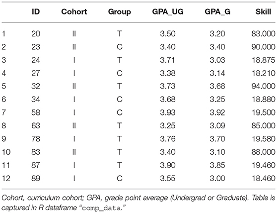
Table 1. Demographic data pertaining to students non-compliant with study protocol.

Computing descriptive statistics for this sub-group is a straight-forward three-step process: (1) set the working directory, (2) read in the data from file, and (3) analyze.

# set the working directory

setwd(″/Users/Docs/Frontiers_Manuscript/

        Code")

# read-in the data from file

comp_data=read.csv(″Frontiers_1

        _SubSample.csv″,

        head=TRUE, stringsAsFactors=TRUE)

# analyze and report

print(paste(nrow(comp_data),

        ″non-compliant students″))

Note the two optional arguments in read.csv. By stating head = TRUE, R recognizes that the dataset contains a header, i.e., “ID,” “Group,” and so-on, are not mistaken for data points; and stringsAsFactors = TRUE forces the columns containing only character (and not numerical) data to be taken as a factor, as might be relevant to statistical analysis. This is helpful even in assessing descriptive statistics, given the summaryBy command (among others).

We note that .csv (comma-separated values) is a common file format for storing numerical data. While we refer to .csv files in this manuscript, R has the ability to open data in a wide variety of formats, included tab-delimited (.txt) and documents prepared in common spreadsheet softwares (i.e., .xls and .xlsx).

The last line of code contains one command nested in the other. This is an entirely legitimate maneuver, and may be quite common amongst experienced coders. The R compiler will read from the inside-out. The nrow(data) function counts the number of rows in the dataset. The paste command attaches a number variable (the number of rows) onto a string variable (the characters in quotes). The print command displays this information on the command line for easy viewing.

The result of this code is a single line report

″12 non-compliant students″

We report the average GPA in this group similarly:

# compute average GPA across sub-group

mean_gpa = round(mean(comp_data$GPA_UG), 1)

stdv_gpa = round(sd(comp_data$GPA_UG), 1)

print(paste(″Average GPA:″, mean_gpa,

        ″+/-″, stdv_gpa))

which yields

″Average GPA: 3.6 +/- 0.2″

In just a few commands, we can visualize these data. For example, suppose we wish to show grade-point distribution as a function of cohort

# show GPA as box plots (break-out by

   cohort)

boxplot(GPA_G~Cohort, data = comp_data)

title(main = ″GPA by Cohort″)

title(ylab = ″Grade-Point Average″)

The plot can be seen in Figure 1A. And while accurate, the visualization may not quite be suitable for publication. We can add a few additional arguments to increase the visual appeal

# modify box-plot for visualization

boxplot(GPA_G~Cohort, data = comp_data,

        names = c(″CohortI″, ″CohortII″),

        ylim = c(1.9, 4.1), cex.axis = 1.5,

        lwd = 3, col = c(″grey50″,

        ″grey80″))

title(main = ″GPA by Cohort″, line = 1,

        cex.main = 2, font.main = 1)

title(ylab = ″Grade-Point Average″,

        line = 2.5, cex.lab = 2)

FIGURE 1

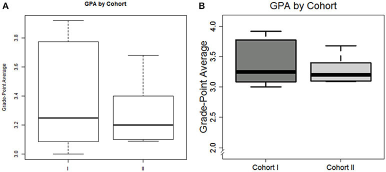
Figure 1. Default plot (A) and modified plot (B) depicting the distribution of graduate GPA amongst non-compliant students in box plot format.

We leave it to the reader to thoroughly inspect the code, but summarize as follows: tick labels are customized for interpretability, the limits of the y-axis is re-defined, the tick fonts (cex.axis) are increased by 50%, the lines comprising the box plot are darkened, and shades of gray are added to the boxes; the title and axis label are re-positioned and re-configured.

Lastly, we note that both the default axis and our own re-definition, places the axis away from zero. In many cases, it may be desirable to “force” the visualization that includes the zero-point. While Base-R does not provide this functionality, the plotrix library does.

library(plotrix)

axis.break(axis = 2, 1.925, style =

            ″slash″)

The final graph can be seen in Figure 1B. Note that this figure can be saved to file from within the R workspace by placing png(″Figure_1b.png″) ahead of the boxplot command, and dev.off() below the last plotting code.

Conditions

It is often desirable to subset the data somehow. Consider the set of data pertaining to non-compliant students (Table 2). Suppose we wanted to isolate just the students with Graduate GPA over 3.50. We first identify those students meeting the GPA criterion with a single line of interrogative code

# test for students exceeding undergrad GPA

threshold

comp_data$GPA_UG > 3.5

TABLE 2

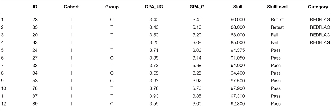
Table 2. Demographic data with adjusted skill scores, factored skill level, and re-sorted based on Red Flag status.

This will return a series of Boolean responses (binary True or False):

FALSE FALSE TRUE FALSE TRUE TRUE TRUE FALSE

TRUE FALSE TRUE TRUE

In order to extract the rows where this condition is met, we use the which function

# return rows reflecting to hi undergrad GPAs

which(comp_data$GPA_UG > 3.5)

      3   5   6   7   9   11   12

To find items exactly meeting a criterion, use the double-equals (voices as “is equals to”) ==

# find which students are in Cohort I

which(comp_data$Cohort == "I")

     3   4   6   7   9   11   12

To find items within a range, it is useful to leverage some of R's set operators (e.g., intersect) and apply multiple conditions

# find students with both GPAs above 3.4

intersect(which(comp_data$GPA_UG > 3.4),

which(comp_data$GPA_G > 3.4))

     5   7   9   11

Dataset Manipulation

There are several useful tools for creating and manipulating categorical variables in R. Consider the same example of students in Table 1. Suppose we wish to flag students with lower-tier scores in skills check. Firstly, we observe that the two Cohorts have scores reported in different scales. We re-scale using the Conditions methods, as in section Conditions:

# convert skill from 20-points to 100%

scale in Cohort I

inds_coh1 = which(comp_data$Cohort == ″I″)

comp_data$Skill[inds_coh1] =

comp_data$Skill[inds_coh1] * 5

We can then convert to a categorical variable via the cut function. Suppose we have three tiers: < 85 points (Failure), between 85 and 90 points (Retest) and 90 or more points (Pass):

# convert skill to leveled variable

comp_data$SkillLevel = cut(comp_data$Skill,

      c(0,85,90,100), labels = c(″Fail″,

      ″Retest″, ″Pass″))

Suppose further that we want to convert this into a 2-level category: those who require follow-up (a Red Flag) and those who do not. We can initialize an column of empty values (default: no follow-up required), and then

# re-level factor variable

comp_data$Category = rep("",

      nrow(comp_data))

comp_data$Category[comp_data$SkillLevel

      %in% c(″Fail″, ″Retest″)]

      = "REDFLAG"

The %in% operator, posed as A %in% B returns Boolean values according to whether each item in A appears in B:

TRUE TRUE FALSE FALSE FALSE FALSE FALSE

TRUE FALSE TRUE FALSE FALSE

Thus, four students require follow-up. To sort these to the top, we re-order the data-frame using

order(comp_data$Category) as a re-sorting vector:

# sort data-frame based on Red Flag status

comp_data = comp_data

            [order(comp_data$Category,

             decreasing = TRUE),]

The phrasing data[inds,] sorts all columns (the empty space between the command and the closing square bracket) according to the indices specified in inds. We can execute a multi-layer sort by adding additional items serially within order:

# sort on Red Flag; sub-sort on Skill Level

comp_data = comp_data

            [order(comp_data$Category,

             comp_data$SkillLevel,

             decreasing=TRUE),]

This modified dataset is shown in Table 2.

Diagnostics

Outliers

Take as a new example the data collected by our group in our studying the impact of video-guided self-reflection as an adjuvant strategy in supplement to the conventional pedagogical strategy in the graduate curriculum. Students from two graduate cohorts were recruited, yielding 25 students with complete results. Here, we show a subset of outcomes, viz. the Academic Locus of Control–Revised questionnaire [ALC-R (Curtis and Trice, 2013)], measured early- (ALC_1) and late (ALC_2) in the semester. Cohort, undergraduate GPA and graduate GPA were noted (Table 3).

TABLE 3

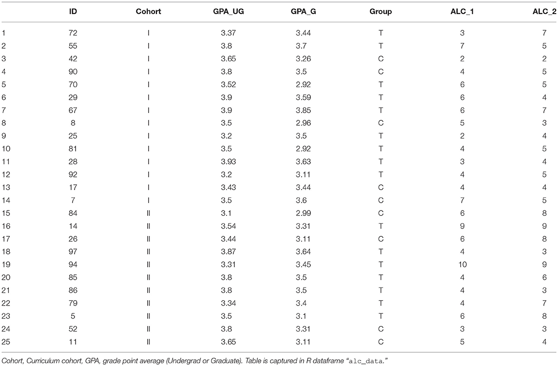
Table 3. Responses to academic locus of control (ALC) questionnaire 15 weeks apart.

Load in this dataset as follows:

# read-in alc dataset

alc_data = read.csv(″Frontiers_2_

             ALCData.csv″, head = TRUE,

             stringsAsFactors = TRUE)

It is typical to identify outliers in a dataset. R can do this efficiently via sub-functionality on the boxplot command:

# identify outliers

boxplot.stats(alc_data$GPA_G)$out

boxplot.stats(alc_data$GPA_UG)$out

where the dollar sign retrieves the outliers (“out”) from the data frame that resulted from the boxplot.stats command. As it turns out, there are no outliers in our dataset with regard to GPA; R returns numeric(0) in both cases. If this seems unlikely, we can confirm by inspection of the data itself. Consider the “z-normalization” transform, i.e., standardization by subtraction of the mean and division by the standard deviation. R performs this via the scale command. Taking the range (min and max) of both datasets, we see:

# double-check outliers via standardization

range(scale(alc_data$GPA_G))

          −1.642978  1.880937

range(scale(alc_data$GPA_UG))

          −1.942531  1.458947

Thus, there are no GPA values that are more than two standard deviations departed from the mean. There are no outliers to remove.

Linearity

Single variables

While we might want to jump right into hypothesis testing, it is prudent to perform some diagnostics first. For instance: while we might wish to test for differential effects, but accounting for academic preparation as co-variate information. Our study collected both undergraduate- and graduate GPA; if they are highly collinear, it would be imprudent to account for them both. We can assess collinearity visually (assessment for a straight-line trend, by inspection), or numerically, via Pearson's correlation. Generating a plot is simple:

# generate a scatter plot of GPA datasets

plot(alc_data$GPA_UG, alc_data$GPA_G,

main = ″″,xlab = ″″,ylab = ″″)

title(main=″Scatterplot of GPA″)

title(xlab=″Graduate GPA″)

title(ylab=″Undergraduate GPA″)

This plot is shown in Figure 2A. Note that R will add default labels to the data unless they are specifically overwritten as empty values (main = ″″,xlab = ″″,ylab = ″″). It is possible to integrate these commands (specifying our custom labels within the plot() command; but we break these commands apart here for clarity. While the figure itself is very helpful, it is not quite publication-ready. We can plot with customized formats, and overlay the correlation value with a few embellishments:

# modify scatterplot for visualization

plot(alc_data$GPA_UG, alc_data$GPA_G,

    main = ″″, xlab = ″″, ylab = ″″,

    pch = 21, lwd = 2, cex = 2,

    col = ″darkblue″, bg = ″lightgreen″,

    ylim = c(1.9,4.1))

title(main = ″Scatterplot of GPA″, line=1,

    cex.main=2, font.main=1)

title(xlab=″Graduate GPA″, line=3,

    cex.lab=2, font.main=1)

title(ylab=″Undergraduate GPA″,

    line=2.5, cex.lab=2, font.main=1)

linmod=lm(GPA_G~GPA_UG,data= alc_data)

abline(linmod)

axis.break(axis = 2, 1.925, style =

   ″slash″)

rho_val = round(cor(alc_data$GPA_UG,

    xalc_data$GPA_G), 2)

text(3.1, 4, paste(″Correlation = ″,

    rho_val), adj = c(0,0), cex=1.4)

FIGURE 2

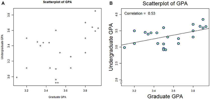
Figure 2. Default plot (A) and modified plot (B) depicting scatter of relationship between undergraduate GPA and graduate GPA.

This plot is shown as Figure 2B. Again, we leave it to the reader to work through the code item-by-item, but we summarize as follows: data are plotted as a scatter plot, with filled circles (#21 in the R plot character set, pch), with double the linewidth and double the size vs. default. A linear model (lm) is created to reflect Graduate GPA as a function of (“~”) Undergraduate GPA, and then plotted via abline. Next, the Pearson correlation is computed, rounded to 2 digits, and annotated on the plot at position x = 3.1, y = 4.0, with a 40% larger font than default; the text is adjusted so that the bottom-left of the first character coincides with the specified position.

Multi variable

There are many convenient tools for diagnostics on multi-variate data, as well. We extend the example of single-variate linearity assessment by fabricating a few additional variables. Let GPA_R1, _R2, _R3, and _R4 be randomly-generated number sets meant to look like plausible GPA datasets.

# create two more GPA variables (for exploration)

set.seed(311)

alc_data$GPA_R1=3.0 + runif(nrow(alc_data))

set.seed(311)

alc_data$GPA_R2=2.5 + runif(nrow(alc_data))

set.seed(331)

alc_data$GPA_R3=3.0 + runif(nrow(alc_data))

set.seed(156)

alc_data$GPA_R4=1.0 + runif(nrow(alc_data))

The random numbers are generated via runif; a random sample of uniform distribution and range zero to one is generated with compatible length (same as number of rows in alc_data). The additive constant (3.0, 2.5, or 1.0) is there merely to re-scale the data to a GPA-like dataset. Note the use of set.seed. Most programming languages allow for random numbers sets to be generated in a way that is reproducible. Soliciting runif(100) will generate a new set of 100 random numbers every time the command is entered. However, by setting a specific seed before invoking the random numbers, the numbers will be called from the same distribution each time. In this way, GPA_R1 and GPA_R2, being of the same seed, will be identical; they will differ from _R3 and _R4, which have different seeds.

We shall now subset the data for convenience:

# take as only those columns containing

″GPA″ in their column names

gpa_data = alc_data[,grep(″GPA″,

           names(alc_data))]

We used the grep function (grep = “globally search a regular expression and print”). The grep function takes as its first argument the text to be searched for, and as its second argument the text to be searched in. Thus, within the names of alc_data, find where “GPA” appears. Given that the names of alc_data are ID, Cohort, GPA_UG, GPA_G, Group, ALC_1, ALC_2, GPA_R1, GPA_R2, GPA_R3 and GPA_R4, the grep command returns {3, 4, 8, 9, 10, 11}. Thus, our subsetting command is equivalent to alc_data[,c(3, 4, 8, 9, 10, 11)], and yields a 25 × 6 matrix of GPA values (some obtained empirically, some fabricated).

We can perform our collinearity assessment through visual means merely by plotting this data frame:

# show scatter

plot(gpa_data, main = ″Collinearity Review

     Scatterplot″)

This plot is shown in Figure 3A. Notice that the plot ticks are scattered: some plot panels show ticks along the top row, some along the bottom; some along the left side, some along the right. For this kind of descriptive assessment, we may prefer to turn off the axis ticks (xaxt and yaxt) altogether. We can add optional arguments to stylize the plot (Figure 3B):

# modify scatterplot for visualization

plot(gpa_data, pch = 21, lwd = 2,

     cex = 1.5, col = ″darkred″, = ″pink″, xaxt = ″n″, yaxt = ″n″)

title(main = ″Collinearity Review

     Scatterplot″, line = 2,

     cex.main = 2, font.main = 1)

FIGURE 3

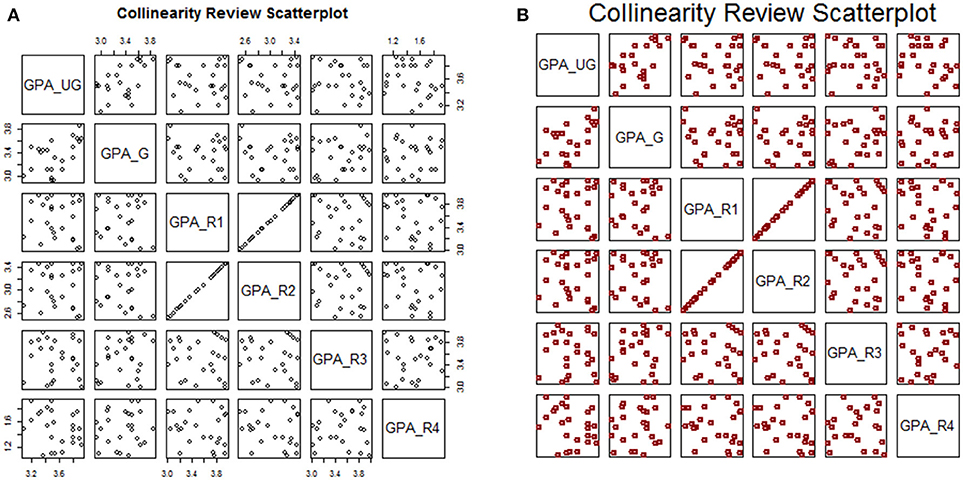
Figure 3. Default plot (A) and modified plot (B) of multi-variate scatterplots for assessing collinearity.

Base-R provides the cor function for calculating the correlation matrix. However, the result is in matrix form, and may not yield easy visualization, especially if there are many variables being compared simultaneously. We can leverage the corrplot package to facilitate visualization of high-dimensional correlation data.

# show correlation matrices

library(corrplot)

corrplot(cor(gpa_data))

title(main = ″Correlation Heat Map″)

This is shown in Figure 4A. We can add additional features to make the plot more print-worthy. Notice that we add a new library for the support of additional graphical devices, i.e., the color ramp palette, which ramps between any number of designated colors (here: red to white to blue)

# modify correlation plot for visualization

library(grDevices)

clrs = colorRampPalette(c(″red″, ″white″,

       "blue"))

corrplot(cor(gpa_data), col = clrs(10),

       addCoef.col = ″white″, number.digits

       = 2, number.cex = 0.75, tl.pos = ″d″,

       tl.col = ″black″, type=″upper″)

title(main=″Correlation Heat Map″, line=1,

       cex.main=2, font.main=1)

FIGURE 4

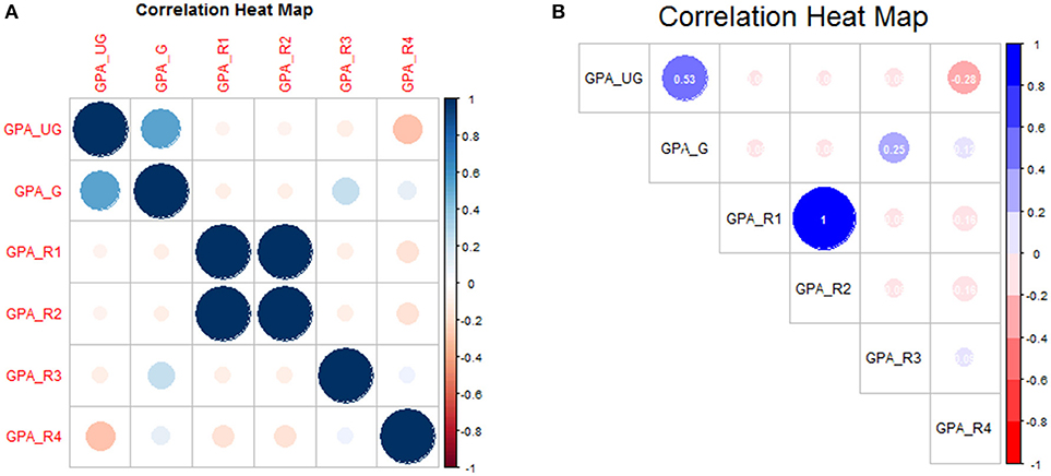
Figure 4. Default plot (A) and modified plot (B) of correlation matrices of multi-variate GPA data.

Again we leave it to the reader to fully explore the code as presented, but summarize as follows: a three-color palette was defined (clrs), and correlation coefficients were added in white text with two-digit precision at 75% default font size. The text label (tl) position was defined to appear along the diagonal (“d”) in black text, and only the upper-triangle of the (symmetric) matrix is shown. The modified correlation matrix is shown in Figure 4B.

Hypothesis Testing

Univariate

A common approach to hypothesis testing for assessment of a single factor is the t-test. Consider a pre- and post-test, for example the Achievement Goal Questionnaire-Revised [AGQ-R (Elliot and Murayama, 2008)], as shown in Table 4.

TABLE 4

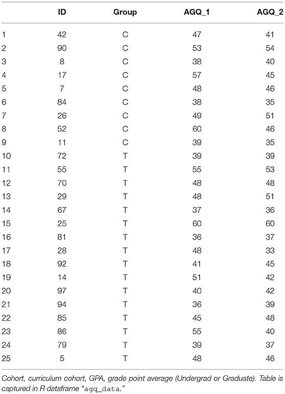
Table 4. Responses to achievement goal questionnaire (AGQ) 15 weeks apart.

A first line of inquiry might be: do students –irrespective of cohort– show an improvement in the AGQ-R after a 15 weeks period. We read-in the data, and can assess statistical significance straight away:

# read-in agq dataset

agq_data = read.csv(″Frontiers_3_

              AGQData.csv″, head = TRUE,

              stringsAsFactors = TRUE)

# paired t-test

pre=agq_data$AGQ_1

post=agq_data$AGQ_2

t.test(pre, post, paired=TRUE)

Note that the optional argument “paired=TRUE” enforces that this is not merely a two-sample t-test with identical sample sizes, but that the measurements are paired. The output reports the t-value (2.24), the degrees of freedom (here: 24, i.e., 25 minus 1), and p-value (0.034). Thus, by frequentist conventions, there is a statistically significant difference post- vs. pre. For more informative view, we compute the summary statistics:

# report differences

print(paste(″AGQ Pre = ″,round(mean(pre),

      1), ″+/-″, round(sd(pre),1)))

print(paste(″AGQ Post = ″,round(mean(post),

      1), ″+/-″, round(sd(post),1)))

Which yields

″AGQ Pre = 46.2 +/- 7.6″

″AGQ Post = 43.6 +/- 6.8″

This is a curious result, so we assess each treatment group independently:

pre=agq_data$AGQ_1[which(agq_data$Group ==

      ″C″)]

post=agq_data$AGQ_2[which(agq_data$Group ==

      "C")]

t.test(pre, post, paired=TRUE)

and

pre=agq_data$AGQ_1[which(agq_data$Group ==

      ″T″)]

post=agq_data$AGQ_2[which(agq_data$Group ==

      ″T″)]

t.test(pre, post, paired=TRUE)

yields, in both cases, a difference that is not statistically significant: for the control group: difference on means of 4.0, 95% Confidence Interval {–0.46, 8.46}, P = 0.07; for the treatment group: 1.88 (–1.31–5.06), P = 0.23. This suggests there may be some value to a multi-variate analysis.

Multivariate

Adding new dimensions to the data can provide greater insight in cases where univariate analysis proves limiting. As a first step, we modify our dataset slightly in order to make for efficient coding:

# convert dataset for multi-variate

analysis

agq_data$Change = agq_data$AGQ_2 -

agq_data$AGQ_1

The only change here is in defining a single variable to report change in score (post-minus-pre). For comfort, verify that the single-sample t-test yields the same result as shown for the same data in the paired-test configuration, i.e., difference on means of 2.64, P = 0.034.

# demonstrate that t-test is the same as

paired test

t.test(agq_data$Change)

Now, consider re-configuring as a one-way ANOVA. We use the same functional notation: aov(Change~Group,data=agq_data), which produces its own output report. But often, the information available through the summary function is more direct, so we wrap aov in the summary command, and name it so that we may extract the p-value efficiently:

# report p-value

aov_summ=summary(aov(Change~Group,

           data=agq_data))

print(paste(″P-value, for AGQ change=″,

      round(aov_summ[[1]][1,5], 3)))

Which yields P = 0.398. We note that the summary of an ANOVA in R is of class type list. Lists may contain matrices, but the matrix contents cannot be extracted directly, the list item has to be extracted first. The list item is extracted by double braces (first list item by [[1]]; nth item by [[n]]…). Since the first item is a matrix (data frame, really), we can then reference it with the conventional matrix references, i.e., [row, column]. Since the first row, fifth column is the P-value associated with the group term, we extract it as aov_summ[[1]][1,5].

In order to add new information, consider merging the co-variates provided through the ALC-R dataset. R contains several helpful tools for merging datasets. We highlight one here, the merge function, available through base R.

# merge AGQ dataset onto ALC dataset for

co-variates

agq_data=merge(agq_data, alc_data)

We can now assess this more informative dataset with an ANOVA where each variable is accounted for:

# test with full anova

aov(Change~Cohort+Group+GPA_UG+GPA_G,

    data=agq_data)

We see from the summary:

# report summary of the anova

summary(aov(Change~Cohort+Group+

        GPA_UG+GPA_G,data=agq_data))

        Df  Sum Sq  Mean Sq  F value  Pr(>F)

Cohort  1  16.1     16.10    0.455    0.507

Group   1  25.7     25.74    0.728    0.404

GPA_UG  1  76.8     76.80    2.172    0.156

GPA_G   1  6.0      5.98     0.169    0.685

Thus it is evident that there are no main effects of significance (P-values for all terms >0.05). It is beyond the scope of this article to address the discrepancy between the two tests; rather, the reader is referred on to more foundational statistics texts for the assumptions of t-tests vs. ANOVA, and encouraged that R has tools built in to help decide which test is most appropriate on a given dataset. Rather, we emphasize here that ANOVA is easily applied in R, and the results easily interpreted.

Lastly, we note that interactions are readily assessed in R, by swapping the additive syntax (+) to multiplicative (*): including an interaction term between, say, Cohort and Graduate GPA is a simple re-arrangement of terms:

# test with anova with an interaction term

summary(aov(Change~Cohort+GPA_UG+

        Group*GPA_G,data=agq_data))

which yields

        Df   Sum Sq  Mean Sq  F value   Pr(>F)

Cohort  1    16.1    16.10    0.441     0.514

GPA_UG  1    67.2    67.15    1.840     0.191

Group   1    35.4    35.38    0.970     0.337

GPA_G   1    6.0     5.98     0.164     0.690

Group:

GPA_G   1    13.8    13.81    0.378     0.546

Where the last row in the summary reports the summary for the interaction term.

Categorical

There are a multitude of tools in R for facilitating hypothesis testing in categorical data. For brevity, we discuss a simple example, that of a 2 × 2 table. Consider the AGQ-R data, with a grouping threshold of those who decreased in AGQ-R vs. those who remained at the same score or improved over time. We start by identifying students who meet each of the strata

# identify the students in each stratum

cohort_1=which(agq_data$Cohort == ”I“)

cohort_2=which(agq_data$Cohort == ”II“)

agq_incr=which(agq_data$Change < 0)

agq_decr=which(agq_data$Change >= 0)

and prepare each cell in the contingency table:

# determine cell values for a contingency

table

agq_cell1=length(intersect(cohort_1,

             agq_incr))

agq_cell2=length(intersect(cohort_2,

             agq_incr))

agq_cell3=length(intersect(cohort_1,

             agq_decr))

agq_cell4=length(intersect(cohort_2,

             agq_decr))

Lastly, we create the contingency table, furnish row- and column-names for the sake of clarity, and perform our hypothesis test:

# create the contingency table, test two

ways

agq_table=matrix(c(agq_cell1,agq_cell2,

            agq_cell3,agq_cell4),nrow=2)

rownames(agq_table) = c(″Cohort_I″,

            ″Cohort_II″)

colnames(agq_table) = c(″Increase″,

            ″Decrease″)

chisq.test(agq_table)

fisher.test(agq_table)

Our contingency table had the structure of

          Increase  Decrease

Cohort_I  6         8

Cohort_II 7         4

And neither the Chi-Square test (P = 0.5293), nor its small-sample alternative, Fisher's Exact Test (P = 0.4283) yielded significance. This matches expectation based on the highly non-diagonalized nature of the contingency table.

Extraction of odds ratios and confidence intervals are straight-forward. We note also that R can handle n-way contingency tables (3 × 3, 4 × 4, etcetera).

Modeling

Linear Regression

Perhaps the most commonly-used methodology for modeling the relationship between two- or more variables is through regression. Here, we demonstrate regression models on these datasets. Firstly, consider Figure 2, showing the relationship between Undergraduate and Graduate GPA. These variables appear to have an approximately linear relationship, so we model as a linear regression:

# read-in alc dataset

alc_data = read.csv(″Frontiers_2_

            ALCData.csv″, head = TRUE,

            stringsAsFactors = TRUE)

# perform linear regression

linmod = lm(GPA_UG~GPA_G,data=alc_data)

Calling this variable from the command prompt yields an output with two items: a summary of the call function, and a listing of the coefficients. Since we specified a simple regression equation, there are only two coefficients: the slope (0.494) and the intercept (1.917). Similarly to the ANOVA, a more informative review of the model can be obtained through the summary command:

# summarize the linear regression

summary(linmod)

which yields, among other things,

Estimate    Std.     txy2     Pr(>|t|)

            Error    value

(Intercept) 1.9174   0.5482  3.4980.00194

GPA_G       0.4940   0.1630  3.0310.00594

At the bottom of the output from the summary, it should be noted that the p-value for the model is p = 0.005939. To connect this to our first look at this dataset, recall that we computed the correlation coefficient via cor (yielding 0.53). We can obtain the statistical significance for that p-value via cor.test(alc_data$GPA_G, alc_data$GPA_UG): p = 0.005939, i.e., the same value obtained through linear regression.

Of course, correlation is a one-dimensional calculation; regression can include many parameters through use of the addition (+) or multiplication (*) notation, see again: section on multi-way ANOVA including interaction terms (above).

Logistic Regression

Logistic regression is used to test predictors of a binary outcome. Consider the very first example presented here, i.e., the sub-group of non-compliant students. Suppose we wanted to determine whether there were any factors that might predict participation vs. non-compliance. We start by reading in the data brand new:

# merge compliant versus non-compliant

data_nonc=read.csv(″Frontiers_1_

            SubSample.csv″, head = TRUE,

stringsAsFactors = TRUE)

data_comp=read.csv(″Frontiers_2_

            ALCData.csv″, head = TRUE,

            stringsAsFactors = TRUE)

and perform a brief quality-control assessment to ensure that there are no common students between the group that participated in the study vs. those that did not:

# verify that there is no overlap between

datasets

olap=intersect(data_nonc$ID, data_comp$ID)

if (length(olap)==0){

      print(″Data Quality Check OK″)

}else{

      print(″Data Error: Non-distinct

             datasets″)

}

We note that this quality check used a new technique: control structure. More about that in a subsequent section (see below).

Because we want to test compliance as a single parameter shared between these two datasets, we must merge them into a single dataset. Firstly, create a new parameter (call it “Status”)

# bind an indicator for compliant versus

non-compliant

data_nonc$Status = ″Noncompliant″

data_comp$Status = ″Compliant″

and subset the two datasets to the same variables

# re-configure variable lineups

data_nonc=subset(data_nonc,

select=c(″ID″,″Cohort″,″Group″,″GPA_UG″,

          ″GPA_G″,″Status″))

data_comp=subset(data_comp,

select=c(″ID″,″Cohort″,″Group″,″GPA_UG″,

          ″GPA_G″,″Status″))

These datasets are now ready for merger by row-binding:

# merge datasets

data_stat=rbind(data_nonc, data_comp)

The Status variable is more likely than not going to be viewed by R as a character variable, given that it was constructed by entering strings. But a logistic regression requires the dependent variable to be factor. Force this class through as.factor:

# enforce classes

data_stat$Status=as.factor(data_stat$Status)

Now, a logistic regression is possible.

# set up a logistic regression

logmod=glm(Status~GPA_G+GPA_UG,

          data=data_stat,family=binomial)

which yields (through summary(logmod)):

             Estimate Std.   z        Pr(>|t|)

                      Error  value

(Intercept)  −2.3298  5.6412 −0.413  0.680

GPA_G        −0.1772  1.5685 −0.113  0.910

GPA_UG       0.6109   1.9398 0.315   0.753

from which it can be concluded that neither undergraduate, nor graduate GPA is significant in its association with compliance in participation.

Mixed Effects

One additional approach worthy of mention is mixed effects modeling, where a process is believed to contain both fixed and random effects. Consider, for example, that our logistic regression model contains graduate students from a diverse set of backgrounds, i.e., various undergraduate institutions and degree programs, and perhaps the students had various levels of engagement during their undergraduate careers. In this setting, and following the constructs of LaMotte (Roy LaMotte, 2006) it is reasonable to believe that the undergraduate GPA might be considered a random effect in slope. We load the library containing mixed effects resources, and reconstruct the logistic regression model with a slight rephrasing of the GPA_UG term:

# load library for mixed effects modeling

library(lme4)

# set up a mixed effects logistic

regression

logmod2=glmer(Status~GPA_G+(1|GPA_UG),

        data=data_stat,

family=binomial)

where the parentheses in the (1|GPA_UG) term flag that variable for random effects, and the 1| indicates that the variable is random in slope (0| would indicate random in intercept). Otherwise, the syntax for performing and obtaining results from mixed models is generally the same as for conventional models. Note that the syntax for a mixed effects models is almost identical to that of a conventional linear- or logistic regression: the first argument in the Response ~ Predictor(s), but with the addition of a term in parentheses indicating random effects.

Notes

Control Structures

While beyond the intended scope of this article, we briefly follow-up on a concept introduced in section Logistic Regression, i.e., control structures. It is possible to provide R with a set of instructions, and for R to carry out only one action, according to pre-defined criteria. The generic structure is as follows: if (condition){action #1}else{action #2}, however more elaborate, multi-conditional structures are possible using else if. Consider a simplistic example

# simple conditional control structure

gpa_val=3.5

if (gpa_val < 3.6){

      print("Med")

}else if (gpa_val < 3.0){

      print("Low")

}else{

      print("Hi")

}

Surely this loop would have no conceivable utility in an actual analytical code, but as an example, it shows proper use of if-else, a basic command structure in every coding language. The criteria does not need to be numerical; any logical/Boolean cue will work, ″g″ %in% c(″a″,″b″,″c″,″d″,″e″,″f″,″g″,″h″) will yield a TRUE.

Perhaps the most common iterative loop structure is the for-loop. The basic structure is for (sequence){action}. A simple example would be

# simple for-loop

for (i in 1:5){

     print(paste(″This is loop number ″, i,

sep=″″))

}

      This is loop number 1

      This is loop number 2

      This is loop number 3

      This is loop number 4

      This is loop number 5

The for-loop can be very powerful: it is possible to perform the same action many times through use of a for-loop, especially when a conditional logic is nested within. For instance:

# scroll through each record and report

red-flag students

for (i in 1:nrow(comp_data)){

     if (comp_data$Category[i] == ″REDFLAG″){

          print(paste(″Student ″,

                 comp_data$ID[i],

                  ″: Red Flag″, sep=″″))

     }

}

One last control structure bearing discussion is the while-loop: while (condition){action}. This loop is, in some respects, equivalent to a hybrid between the if-loop and the for-loop: it iterates (like a for-loop), until a condition has been met (like an if-loop). The major caveat here is that for a for-loop there is a finite terminus: once the control sequence is exhausted, the loop will cease; for a while-loop, it is possible for the criterion to never be realized, leading the loop to continue ad infinitum (a “runaway”). A runaway loop will seize R; the only remediation is to stop the calculation through the STOP button in the R console, or to brute-force stop the software, e.g., Task Manager.

RStudio

R as described here is intended to convey primarily command-line programming within the traditional R computing environment. The reader may take interest, however, in some of the tool suites available as augmentation or substitute for R, including RStudio. RStudio offers the same functionality of R in computation, but much more accessibility in terms of user interface. Personal license for single-use RStudio or RStudio Server remains free of charge, but there are Commercial packages that unlock additional features including Priority Support.

Other Softwares

It is expected that new users to R will be “immigrating” from other software platforms, or may have need to interface with team members who are utilizing other softwares. There are options for this kind of transfer or exchange. Firstly, there are many guides offering syntactic cross-walk between R and SPSS, SAS, Matlab, etcetera (Muenchen and Hilbe, 2010; Muenchen, 2011; Kleinman and Horton, 2014). But there are also some built-in codeworks that allow for ease of transition. For example, the SASxport library and sub-functions within the Hmisc library. While some functions shall remain –by design– the singular domain of their proprieter, a great many functionalities available in the commonly available statistical softwares can be found in R.

We note, also, that R is not the only open-source computing environment that is popular among data scientists. For instance, Python, is widely used, particularly in the engineering and physical sciences. Historically, Python is considered a more general-purpose language; R is almost always used for statistical analysis. However, both packages have flexibility into both analytical and technical application, and either present many options for those seeking to add a computational edge to their work. For proprietary environments, Matlab has grown its statistical packages incredibly over the past 15 years, and has an incredible plotting engine, and is a de rigueur skills set for nearly every graduating engineer. SAS is considered by many to be the mainline software in clinical trials design and primary analyses, although the US Food and Drug recently clarified that they do not explicitly require the use of any specific software for statistical analysis (Statistical Software Clarifying Statement, 2015). We find that among the commercially available softwares used for statistical analysis, STATA and SPSS are popular with colleagues in the fields of education and allied health. We urge that every software has its plusses-and minuses, but that the open access of R, and its thriving users community, make it highly attractive to the intrepid investigator seeking a useful and portable analytical tool.

Conclusion

In this article, we provide educational researchers with an introduction to the statistical program, R. The examples provided illustrate the applicability of R for use in educational research; these vignettes are designed to be extensible to a broader set of problems that interest those in educational research. While numerical programming is not typically the province of the educational researcher, we urge that it is easy to get started, and that there is excellent support for those wishing to integrate R into their analytical repertoire.

Data Availability Statement

The datasets included in this study can be found as supplements to this manuscript.

Ethics Statement

Data presented in this manuscript were collected in a protocol approved by the Human Subjects Committee at the University of Hartford. All participants gave written informed consent prior to study participation.

Author Contributions

Code creation: Led by MW, reviewed and approved by TP. Data collection: Led by TP, consulting with MW. Manuscript creation: Tandem effort by MW and TP.

Funding

The authors acknowledge the College of Education, Nursing and Health Professions, University of Hartford, for grant support in completion of this manuscript.

Conflict of Interest Statement

The authors declare that the research was conducted in the absence of any commercial or financial relationships that could be construed as a potential conflict of interest.

Supplementary Material

The Supplementary Material for this article can be found online at: https://www.frontiersin.org/articles/10.3389/feduc.2018.00080/full#supplementary-material

References

Bishop-Clark, C., and Dietz-Uhler, B. (2012). Engaging in the Scholarship of Teaching and Learning: A Guide to the Process, and How to Develop a Project From Start to Finish. 1st edn. Sterling, VA: Stylus Publishing, LLC.

Google Scholar

Boyer, E. L. (1997). Scholarship Reconsidered: Priorities of the Professoriate. 1st edn. Princeton, NJ: Carnegie Foundation for the Advancement of Teaching.

Google Scholar

Curtis, N. A., and Trice, A. D. (2013). A Revision of the Academic Locus of Control Scale for College Students. Percept. Mot. Skills 116, 817–829. doi: 10.2466/08.03.PMS.116.3.817-829

PubMed Abstract | CrossRef Full Text | Google Scholar

Elliot, A. J., and Murayama, K. (2008). On the measurement of achievement goals: Critique, illustration, and application. J. Educ. Psychol. 100, 613–628. doi: 10.1037/0022-0663.100.3.613

CrossRef Full Text | Google Scholar

Gilpin, L. S., and Liston, D. (2009). Transformative education in the scholarship of teaching and learning: an analysis of SoTL literature. Int. J. Scholarsh. Teach. Learn. 3:11. doi: 10.20429/ijsotl.2009.030211

CrossRef Full Text | Google Scholar

Hutchings, P., Huber, M., and Ciccone, A. (2011). Feature essays: getting there: an integrative vision of the scholarship of teaching and learning. Int. J. Scholarsh. Teach. Learn. 5:31. doi: 10.20429/ijsotl.2011.050131

CrossRef Full Text | Google Scholar

Kanuka, H. (2011). Keeping the scholarship in the scholarship of teaching and learning. Int. J. Scholarsh. Teach. Learn. 5:3. doi: 10.20429/ijsotl.2011.050103

CrossRef Full Text | Google Scholar

Kleinman, K., and Horton, N. J. (2014). SAS and R: Data Management, Statistical Analysis, and Graphics. 2nd edn. Boca Raton, FL: CRC Press, Taylor & Franciss Group.

Google Scholar

Martin, R. C. (Ed.) (2009). Clean Code: A Handbook of Agile Software Craftsmanship. Upper Saddle River, NJ: Prentice Hall.

Google Scholar

Mertens, D. M. (2014). Research and Evaluation in Education and Psychology: Integrating Diversity With Quantitative, Qualitative, and Mixed Methods, 4th Edn. Sage Publications, Inc.

Google Scholar

Muenchen, R. A. (2011). R for SAS and SPSS Users. 2nd edn. New York, NY: Springer.

Google Scholar

Muenchen, R. A., and Hilbe, J. M. (2010). R for Stata Users. New York, NY: Springer.

Google Scholar

Osborne, J. M., Bernabeu, M. O., Bruna, M., Calderhead, B., Cooper, J., Dalchau, N., et al. (2014). Ten simple rules for effective computational research. PLoS Comput. Biol. 10:e1003506. doi: 10.1371/journal.pcbi.1003506

PubMed Abstract | CrossRef Full Text | Google Scholar

Prlić, A., and Procter, J. B. (2012). Ten simple rules for the open development of scientific software. PLoS Comput. Biol. 8:e1002802. doi: 10.1371/journal.pcbi.1002802

PubMed Abstract | CrossRef Full Text | Google Scholar

Roy LaMotte, L. (2006). “Fixed-, random-, and mixed-effects models,” in Encyclopedia of Statistical Sciences, eds. S. Kotz, C. B. Read, N. Balakrishnan, B. Vidakovic, and N. L. Johnson (Hoboken, NJ: John Wiley & Sons, Inc.).

Google Scholar

Statistical Software Clarifying Statement (2015). United States: Food & Drug Administration. Available online at: https://www.fda.gov/downloads/ForIndustry/DataStandards/StudyDataStandards/UCM587506.pdf (Accessed August 13, 2018).

Thieme, N. (2018). R generation. Significance 15, 14–19. doi: 10.1111/j.1740-9713.2018.01169.x

CrossRef Full Text | Google Scholar

TIOBE (2018). TIOBE Index for March 2018 (Eindhoven, Netherlands). Available online at: https://www.tiobe.com/tiobe-index/ (Accessed March 19, 2018).

Willems, K. (2014). What is the Best Statistical Programming Language? Infograph. Available online at: https://www.datacamp.com/community/tutorials/statistical-language-wars-the-infograph (Accessed March 19, 2018).

Wilson, G., Aruliah, D. A., Brown, C. T., Chue Hong, N. P., Davis, M., Guy, R. T., et al. (2014). Best practices for scientific computing. PLoS Biol. 12:e1001745. doi: 10.1371/journal.pbio.1001745

PubMed Abstract | CrossRef Full Text | Google Scholar

Witman, P. D., and Richlin, L. (2007). The status of the scholarship of teaching and learning in the discipline. Int. J. Scholarsh. Teach. Learn. 1:14. doi: 10.20429/ijsotl.2007.010114

CrossRef Full Text | Google Scholar