 Pascal Kilian
 Frank Loose
 Augustin Kelava
- 1Methods Center, University of Tübingen, Tübingen, Germany
- 2Tübingen School of Education, University of Tübingen, Tübingen, Germany
- 3Department of Mathematics, University of Tübingen, Tübingen, Germany
In math teacher education, dropout research relies mostly on frameworks which carry out extensive variable collections leading to a lack of practical applicability. We investigate the completion of a first semester course as a dropout indicator and thereby provide not only good predictions, but also generate interpretable and practicable results together with easy-to-understand recommendations. As proof-of-concept, a sparse feature space together with machine learning methods is used for prediction of dropout, wherein the most predictive features have to be identified. Interpretability can be reached by introducing risk groups for the students. Implications for interventions are discussed.
Introduction
High dropout rates in mathematics and general in the STEM fields (science, technology, engineering and mathematics)—more precisely, in Germany, the so-called MINT disciplines (mathematics, informatics, science and technology)—are not a new phenomenon. According to Heublein (2014), in Germany 39% of the students in MINT disciplines drop out of the Bachelor program. Compared to the German general average of 33% this is a rather high dropout rate. In mathematics, the dropout rate is even higher with 47% (U.S. college dropouts show comparable numbers; Chen, 2013). In contrast to the MINT dropout rates during the bachelor, the 5% dropout rate during the master is much lower (Heublein, 2014). Thus, this paper focuses on the investigation of the initial phase of the study program, more precisely the Analysis 1 (Calculus 1) lecture which is a typical (and mandatory) start in the mathematics study program. This means the subject of research in this paper is not dropouts (from university or the study program) but dropouts and success in this lecture in the sense of a non-completion rate. We see that as a strong indicator for possible future dropouts. A detailed definition of the non-completion (of Analysis 1) variable can be found in the methods section. For the sake of clarity, throughout the rest of the paper we will use the term dropout when talking about the general problem and non-completion for the dependent variable in our study.
The examination of these unusually high dropout rates in MINT disciplines becomes even more interesting and relevant, knowing that those students show high cognitive prerequisites (Nagy, 2007). Nagy showed high correlations of cognitive abilities with realistic and investigative vocational interests (based on the vocational interest model of Holland, 1997) where those disciplines are classified. Excluding low cognitive abilities of the participants, the question arises, why we experience high dropout rates, especially in those disciplines. Included in the high dropout rates in mathematics are those students intending to become math teachers. The lack of those teachers gives additional motivation for decreasing the dropout rates. Since teacher candidates might differ from B.Sc. students (in motivation, academic achievements,.), we will investigate differences between those groups to preclude different prerequisites, different dropout behavior, which would mean different interventions. Teacher candidates will thus be a special focus of this study in the sense that it is important to investigate if they constitute a special case of students which need to be treated accordingly. Furthermore, former studies in this field use large feature spaces by including a very broad range of potential determinants/variables in different areas. Those variables are not available for practical usage on a regular basis, and thus, the models are not useful for practical implementations. We address this problem by using a sparse feature space including only a few variables all of which are cheap to collect at the beginning of a course. Those variables cover areas proved to be related to dropouts. A broader variable collection would improve prediction results but is not feasible on a regular basis, thus in this paper we investigate what can already be achieved with those variables.
Structure of This Paper and Notes
First, in the following section we briefly discuss different theoretical frameworks of college student dropout and results of former studies and summarize the general current state of research. Secondly, we introduce empirical studies more specific to the topic of this paper, followed by thirdly, the design of the present study and the research questions. The methods and results sections follow, and we close with a discussion of our findings.
The goal of this paper is 2-fold. The methods are applied in the German teacher education setting. Thus, one goal is to generate specific results which help to identify risk groups and the planning of intervention. The second goal is to introduce data science methods to educational research.
For example, the U.S. teacher education differs from that in Germany, so specific results might not be relevant and applicable to other universities and systems (due to the system as well as to our limited sample size), but the general ideas and procedures can easily be adapted to those settings.
Current State of Dropout Research
The investigation of dropouts can draw on a high quantity of studies and literature. In terms of dropout related factors, a big variety of variables have been investigated. Variables have been identified on individual, institutional, environmental-related and system-related levels. Following Bean (2005) and Burrus et al. (2013), variables can be classified in (a) institutional environment factors, (b) student demographic characteristics, (c) commitment, (d) academic preparation and success factors, (e) psychosocial and study skill factors, (f) integration and fit, (g) student finances and (h) external pull factors.
In the following we focus on factors within (b) student demographic characteristics and (d) academic preparation and success factors, as these reflect the design of this study best. Examples for student demographic characteristics are, among others, the student's age, sex, race and ethnicity. Feldman (1993) reveals a nonlinear connection between age and student dropout—younger and older students showed higher dropout probabilities. Hagedorn et al. (2001) show a slightly negative effect of age on students' retention. For students' sex no simple linear effects have been described, but interactions with other variables have been shown (e.g., with the existence of children in Leppel, 2002). Academic abilities like school performance measures and general performance measures are examples of the (d) academic preparation and success factors. Standardized tests show the expected high correlation with student's retention at university (e.g., Bean, 2005).
With regard to the mentioned studies, it can be said that a wide range of variables show some connection (correlation) with student dropout, but few variables with singular effects can be found. This indicates a relationship wherein the effect might rely on complex combinations of variables. The motivation arises to expand the approaches from linear models to models which take this complexity into account, for example in prediction models.
The dropout literature relies mostly on two comprehensive frameworks for understanding students' dropout decisions. First there is Tinto's theory of student departure (Tinto, 1975, 1987). A central point of his theory is the students' integration and interaction with the faculty, staff and peers in both academic and social settings (Tinto, 1993; Burrus et al., 2013). The model has been validated and generally adjudged to be a useful framework (e.g., Terenzini and Pascarella, 1980). The second framework is the model of student attrition by Bean (1980, 1983, 2005). This framework implies more external factors, e.g., the expenditure of time, financial resources or the students' responsibility for their families. In both models, the intention to drop out is explained by the variables: contentment with the study program, the pursuit of the final degree and the power of endurance.
More recent approaches focus more on individual characteristics of the students. Schiefele et al. (2007), for example, show that differences between students who dropout and persistent students are mostly found in motivation, social competence, perceived teaching quality, the self-evaluated knowledge state and the use of learning strategies. Keeping in mind the unfeasibility of those large models, in our study we aim to consider variables of diverse areas, but with the practical availability, as well as the possibility for complex modeling.
Considering more technical approaches for various predictions in higher education, our research can be seen in the context of the growing field of educational data mining (EDM). Here, an increasing number of studies for example on the prediction of academic performance and student attrition, using data mining and machine learning approaches, can be found. Alyahyan and Düştegör (2020) review a broad range of articles on academic success prediction, including amongst others the course level, where our research would be located. Successful applications have been published, but nevertheless most of those studies differ from our research in prediction goals and especially in the available data. Pérez et al. (2018) as well as Berens et al. (2019) for example achieve good prediction results only by including information about academic performance during the first semester. This indicates the importance of the academic performance during the first semester and motivates investigations about risk groups at the very beginning of higher education. But for the identification of the risk groups within the first semester, academic performance measures are not yet available.
Math Specific Dropout Research
Several studies, especially for mathematics, have been conducted with focus on the transition from school to university including individual prerequisites (Grünwald et al., 2004; Gueudet, 2008; Eilerts, 2009; Heublein et al., 2009). Parts of the risk factors of those studies can be summarized as student's prerequisites prior to university. Below we discuss some of those prerequisites with special regards to teacher candidates as our focus group.
Regarding the choice of the study program, it seems to be a public opinion that there is a negative selection within the mathematics students toward the teacher candidates. It is assumed that weaker students choose the teacher program Bachelor of Education (B.Ed.) instead of the pure math program Bachelor of Science (B.Sc.). External reasons like occupational safety and longer vacation periods are named motivations for this choice. These reasons might be more important than the motivation of becoming a teacher itself (Blömeke, 2005; Klusmann et al., 2009). Taking this into account, we particularly pay attention to this group of students. Taking this into account, we pay particular attention to this group of students, by investigating possible differences, in the sense of a negative selection (differences in prerequisites), as well as dropout behavior (risk group). However, a negative selection was not found by Klusmann et al. (2009), comparing school grades, cognitive abilities and results of a standardized math test [Third International Mathematics and Science Study (TIMSS, e.g., Baumert et al., 1999)], between teacher candidates for the academic track (B.Ed.) and non-teacher candidates at university (B.Sc.). Those results refer only to measurements at the end of school and give no information about the success at the university. In their study Klusmann et al. (2009) used data of the study Transformation des Sekundarschulsystems und akademische Karrieren (TOSCA; Köller et al., 2004), which does not differ between B.Ed. and B.Sc. students. Besides gender, the analysis was controlled for the field of the study subject (inclusion of at least one subject within the field of science or not). Therefore, the data is not differential enough for statements within the subject of mathematics. Even though the initial prerequisites might be the same, both study programs start to differ vastly already in the first semester. Teacher candidates have to face the double pressure of two majors. Differences in success and dropout or non-completion rates during the semester might occur. Differences in success and dropout or non-completion rates during the semester might occur, which would lead to separate problems and solutions compared to the B.Sc. students. Due to the importance of content knowledge for teaching and its relation to pedagogical content knowledge (e.g., Kunter et al., 2011), it is a critical question if the teacher candidates fall behind their colleagues in terms of success and dropout or non-completion rates already in the first semester.
The Present Research
In this study, we analyze the success in the first semester lecture Analysis 1 (Calculus 1). Within this lecture, we compare the prerequisites of students in different study programs and connect it to the above-mentioned studies (e.g., Klusmann et al., 2009). These prerequisites are then used to predict non-completions in this time period. For a more detailed definition of the term non-completion in this study we refer to the methods section below.
As seen in former studies and frameworks (e.g., Tinto, 1975, 1987, 1993; Bean, 1980, 1983, 2005; Schiefele et al., 2007; Burrus et al., 2013), a broad variety of possible dropout predictors or risk factors can be tested. Even though the different models show overlaps in the sets of risk factors, a common set for practical usage is hard to identify. This shows the complex structure of student dropout and interactive relation of different risk factors. The complexity of the topic gives rise to problems for policy makers. Feasible applications of the research results are limited to the availability of variables. The identification of risk groups (e.g., for interventions or restriction of admission) including the wide range of variables is too expensive and not practical, for example for universities, on a regular basis.
In this study, we use a very small set of possible predictors by only including, (a) data collected at the beginning of the semester (excluding for example performance measures during the semester or different state variables), and (b) variables which can be collected with little cost at the beginning of the lecture. The reasons for this choice are (a) to find risk factors in students' prerequisites excluding the students' behavior during the lecture (e.g., the expenditure of time) and (b) to enable universities to use the results of this study with little cost. We not only use a sparse feature set with a small number of variables, but the data is also limited in sample size. Here, we also refer to the practicality of these methods for universities and propose a course of action to reduce non-completions in practice. In practical application scenarios, limited information about the students of the specific university is common, but even then valuable insights can be attained. Even though the data only contains data from one specific course, which implies limitations for the generalization of specific results, the Analysis 1 course is representative of first semester courses both beyond this university and beyond Germany. We further address this topic in the discussion of this paper. Possible actions could be entrance qualifications and the identification of risk groups early in the program to provide support courses and interventions. The standard method to identify significant risk variables for a binary variable like student dropout or non-completion is the logistic regression. As the logistic regression only works on linear relations, we will use prediction models that are able to take complex interactions into account. This approach aims to be more practical compared to the theoretical approaches discussed above. As shown, risk factors for student dropout can be found in students' personalities, school backgrounds, social and academic integration and many more. Although those broad theoretical approaches are important for the understanding of dropout risk factors, they are not of practical use for universities (in most cases simply because of the inaccessibility of the wide range of variables). In order to enable universities to quickly identify risk groups the focus of this study is the prediction of student non-completion using only a few, leviable variables, in sophisticated models.
Research Question
The research questions of this study can be summarized in three questions.
(R1) Can differences between groups of students be identified at the beginning of university (especially between B.Ed. and B.Sc.) in their prerequisites and in their non-completion behavior, with implications for planned interventions?
(R2) Starting with variables that are easy to obtain at the beginning of the semester, what prediction accuracy can be achieved (upper bound?) with this sparse feature space and can this be further reduced?
(R3) Can the prediction results be used to identify risk groups already at the beginning of the semester?
(R1) and (R3) include the investigations about the group of teacher candidates. In (R1) we focus on prerequisites. (R3) includes the question of whether being a teacher candidate itself leads to a risk classification indicating different dropout or non-completions behavior.
Methods
Study Design and Sample
We examine two consecutive Analysis 1 lectures (cohort 1 and cohort 2) of the University of Tübingen (winter semester 2014/15 and 2015/16). Due to the curriculum, it is mandatory to participate in the Analysis 1 course, for both, B.Sc. and B.Ed. students. In Tübingen, the physics (B.Sc.) students participate in this course in the first semester as well. The schedule of the Analysis 1 lecture is comparable for both cohorts. In addition to attending the lectures, students are divided into small tutorial groups. Within the tutorial groups, students have to submit homework every week. In order to obtain the admission to the final exam, achievements in the context of those tutorials and of the problem sets are relevant. As the cohorts can be seen as a homogeneous sample with respect to the used variables, in the analysis we combine both (dataC) to reduce the dependence on lecturers and lecture schedules and to gain more general results.
Included in the dataset are students which major in mathematics (B.Sc.) or physics (B.Sc.) and mathematics teacher training students (B.Ed.). All of the students did not actively participate in a former Analysis 1 lecture, even though it might not be their first mathematical semester.
Instruments
The dataset contains the results of every student on every problem set, which allows to follow the students' development during the first semester and we can see the exact week of the withdrawal, if students quit. Additionally, the results of the final exams are analyzed. Those results indicate success or failure of the Analysis 1 lecture. For further information about the preconditions of students, like personal data (e.g., age, gender, school grades, study path), a questionnaire was used in the second week of the semester.
In addition to the covariates, the students finished five items of the Third International Mathematics and Science Study (TIMSS, Baumert et al., 1999; Mullis et al., 2007) in the questionnaire. The international scale of TIMSS is set to a mean of 500 with the standard deviation of 100 (Adams et al., 1997). Because we only use a set of five items,1 which are suitable for the contents of the Analysis 1 lecture, we built sum scores of the correct answered items.
About 95% of the students filled in the initial questionnaire. In order to be able to access students' lecture data an additional permission was needed. Ninety-five percentage of the students granted this permission.
As mentioned in the current state of the dropout research, a broad range of variables are related to dropouts. Universities and lecturers typically have no access to exhaustive data sets but have to deal with the available information. The variables introduced here can be seen as a compromise between realistic availability and the full range of relevant information. In our research the focus is on the application of sophisticated algorithms to investigate what results can be achieved with a non-exhaustive data set. Therefore, our variable set can also be seen as an example of available data and should not be interpreted as the best variable selection.
Possible Predictors
With the study design, including the questionnaire, we take into account the following variables as students' attributes for the predictions. Different performance measures from school [“GPA,”2 math grade in the final exam (“math grade”)] and results of the TIMSS items (“timss”), the participants “age” and “sex,” the federal state (“state”) and “school type” in which the university-entrance diploma was received. The variable “school type” indicates if the university-entrance diploma was received at a general-education Gymnasium (academic track), if the participants are teacher candidates (B.Ed.) or not (“tea”), if a prep course for math, prior to the Analysis 1 lecture was attended (“prep”) and if the respective semester was the first semester of a mathematical study program (“first”). The variable “first” includes students which already attended other lectures than the Analysis 1 or already attended the Analysis 1 lecture but did not achieve exam admission and thus cannot be recognized as former Analysis 1 participants.
The dependent variable “pass” indicates the success in the Analysis 1 lecture. For a successful participation in Analysis 1, the participants have to pass the final exam. In Table 1 the descriptive analysis of the variables is outlined for the different data sets.
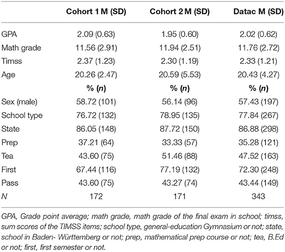
Table 1. Descriptive data for cohort 1, cohort 2 and the combined data set dataC.
Definition of Non-completion and Bounds for Prediction Accuracies
In this study, we use a very simple definition/indicator of dropouts in the Analysis 1 lecture, namely non-completion. Students fail to complete if they fail the Analysis 1 lecture. The participants complete the Analysis 1 lecture if they qualify to take part in the final exam and pass the test. If they don't pass the final exam, they have one more chance in a makeup exam, which is similar to the original test. Thus, there are several ways for non-completion. First, the students can choose to voluntary quit during the semester. Secondly, they might not obtain the admission for the final exam, or thirdly, they don't pass both the final exam and the repeat exam. In this study, we do not differentiate between the different ways of non-completion. We only consider the dichotomous variable pass or not pass.
To gain a better sense of prediction accuracies we discuss some bounds. As a lower bound of the expected prediction accuracy we use a baseline model which predicts a dropout for every example. Due to the “pass” percentage of 43.44% in dataC this will result in an accuracy of 0.57 or 56.56%. Therefore, we can achieve an accuracy of 56.56% with a model that uses no information of the training data and thus builds the lower bound for the accuracies of our models.
The upper bound cannot be specified exactly but we discuss some ideas. As features we only use attributes of the students before they came to university. Therefore, this approach uses no information on the behavior of the students during the semester. But the active participation in lectures and tutorials as well as the general effort of the students is seen to be crucial for the success in math. Therefore, the expected accuracies of our models are far <100%. Even with a sufficient amount of data, including data referring to the behavior during the semester, we would not expect to come close to 100%, because the final exam itself implies uncertainty of success. In conclusion, we expect the accuracies to be better than 57% in order to have a valid predictor, but we do not expect the accuracies to exceed 80% (as an educated guess), due to the uncertainty of the behavior during the semester and in the test situation.
General Analysis
In this part, we discuss general methods and procedures which occur in all the following models and algorithms. More details for the specific algorithms are discussed in the following section. In order to report realistic measures for the prediction quality we divide the data set in a test set and a training set by randomly assigning 20% of the data to the test set. This procedure is performed with cohort 1 and cohort 2. Then the training sets and test sets are combined, respectively, to receive the training set and test set for dataC. The test set remains untouched and unseen until the evaluation of the specific algorithm. This process results in Ntrain = 275 (Ntrain,cohort1 = 138 and Ntrain, cohort 2 = 137) and Ntest = 68 (Ntest, cohort 1 = 34 and Ntest, cohort 2 = 34).
Differences in the Prerequisites for Teacher Candidates
We compare the variable means and frequencies of the B.Ed. students with those of the B.Sc. students. Differences are tested by means of t- and χ2-tests.
Procedure for the Prediction Models
In the prediction models, we train classifiers to predict the target3 “pass.” These are binary classifiers with the positive class referring to passing the Analysis 1 lecture. The general procedure for the predictor models is as follows: We train the model using the training set. If hyperparameters need to be tuned we use cross-validation within the training set. For the model selection, we use different prediction measures using the training set. We report the accuracy on the training set, the leave-one-out cross-classification/validation (loo.cv), and the precision, recall and F1-score values. For model evaluation, we report the same measures, except for the loo.cv, on the separated test set. Note that due to the relatively small size of the test set, we also consider the loo.cv as measure for the generalization error or accuracy. This error is known to be an unbiased estimator for the generalization performance of a classifier trained on m-1 examples (e.g., Rakotomamonjy, 2003; Evgeniou et al., 2004). In addition to the accuracy measures we report Cohen's Kappa as measure for the inter-rater agreement of the predictions and the true outcomes (Cohen, 1960). For the interpretation of Cohen's Kappa, we use the suggestion of Landis and Koch (1977). They define the strength of agreement for kappa values of 0.00–0.20 as slight, 0.21–0.40 as fair, 0.41–0.60 as moderate 0.61–0.80 as substantial and 0.81–1.00 as almost perfect.
For feature selection, we train the biggest model using all available attributes as features, evaluate the prediction measures and check if the evaluation—the quality of the prediction—decreases for smaller models. The detailed feature selection procedures are discussed in the Supplementary Material.
Analysis for the Different Methods
In this part, we give an overview of the methods for the different algorithms and models. We use (i) the basic logistic regression, (ii) logistic regression with elastic-net regularization, (iii) the Support Vector Machine and (iv) tree-based methods for feature selection and prediction. Note that group differences and effects of features are also considered in the prediction models by the independent variables.
Within the methods, specific procedures have to be applied for model and feature selection. We provide further details of the methods (hyperparameter tuning and feature selection) in the Appendix.
Logistic Regression (and Elastic Net Regularization)
Following standard procedures in prediction algorithms, we not only use logistic regression, but also the logistic regression with elastic net regularization (Hastie et al., 2009; Friedman et al., 2010). Introducing regularization advances the algorithm in two ways. First, the (partly) inclusion of L1/lasso-regularization (determined by the tradeoff parameter α) performs a kind of continuous subset or feature selection. Second, by regularization we can reduce the complexity of the algorithm yielding better generalization results on unseen data by reducing overfitting.
Support Vector Machine (SVM)
We use a SVM with linear kernel and the more flexible SVM with radial basis function kernel (RBF kernel). For the analysis we use the R package e1071 (R Core Team, 2015; Meyer et al., 2017). Different feature selection algorithms have to be performed for those algorithms. In the linear case we implement the recursive feature elimination algorithm SVM-RFE. To use SVM-RFE in the non-linear case, the approach can be generalized following (Guyon et al., 2002).
In the linear and non-linear case only the cost parameter C or the cost parameter C and shape parameter γ have to be tuned respectively (following Meyer et al., 2017). Thus, those parameters are reported in the results. Further details are provided in Appendix B. General details on SVMs can be found in Hastie et al. (2009), for example.
Tree-Based Models
We apply tree based models and refer to Hastie et al. (2009) for a detailed general introduction and to Hothorn et al. (2006a,b) for an introduction of the here used conditional inference trees and random forest based on them (Strobl et al., 2007, 2008), implemented in the R package party (Hothorn et al., 2006b; R Core Team, 2015).
In the forest setting we tuned the hyperparameter responsible for the number of features randomly selected in each split (mtry) and report it in the results. Standard values are used for other hyperparameters (Hothorn et al., 2006a; Strobl et al., 2007, 2008).
Feature or variable selection is either included in the general concept (single decision tree) or we use the conditional importance (Strobl et al., 2009).
Further details about the algorithms and the feature selection procedures are given in Appendix C.
Comparison of the Predictors and Risk Groups
In the last step of the analysis we select the best predictors of each method, summarize their results and use them combined as ensemble predictor. For that purpose, we use the predictions of the single predictors and combine them via a majority vote for the class assignment.
We use this ensemble predictor for the identification of risk groups. With the predictions, the data is separated naturally into three groups. The first group consists of the true positive predictions. At last, the third group refers to students with feature vectors that were predicted falsely. Depending on the application, either group two or both group two and three can be defined as the risk group. In this study, we define group two—the true negative prediction—as the risk group. Reasons for this choice are given by the general design of the prediction task. We avoid important information about students' behavior and situation during the semester, but only use information prior to university, thus wrong predictions can be partly associated with the information not included in this study. Therefore, group three—the wrong predictions—refer to the uncertainty during the semester. In that context and at this point we can define the risk group as those students that are, by the prediction model, predicted to fail the lectures with high certainty.
We summarize descriptive measures for the three groups in the results. In order to correctly interpret the results, it is important to define characteristics of the risk group. This can be done by partitioning the feature space and identifying the partitions, which can then be assigned to the risk group. Since this is exactly what the decision tree method does, we apply the already introduced conditional inference tree. For that purpose, we only include features that have been selected as most predictive by the different methods.
Results
In this part, we first report results of the group comparison, especially between B.Ed. and B.Sc. students (R1); secondly, we report the specific and general feature selection results, together with prediction accuracies and compare the different methods we apply (R2); and thirdly, we discuss and describe the identified risk groups (R3).
Differences of Groups of Students at the Beginning of University (R1)
Differences in prerequisites of teachers are shown in Table 2. The non-significant differences in the GPA confirm the results of Klusmann et al. (2009), but we see differences in the selected TIMSS items and the math grade. Those results don't necessarily contradict the results of Klusmann et al. (2009), since our results solely concern the students of mathematics. There are also significant differences in prep and first. Forty-nine percentage of the B.Sc. students attended a mathematical prep course compared to only 20% of the teacher candidates, while at the same time significantly more B.Sc. students are in their first mathematical semester.
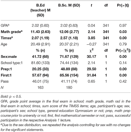
Table 2. Group differences between B.Ed. students (teachers) and B.Sc. students.
Feature Selection Results and Prediction Accuracy (R2)
Features Selection
For the logistic regression with selected features, we first analyzed the complete model and use the significant features—GPA, math grade, timss and first—and the features school type and tea, as their respective p-values (0.07 and 0.05) are close to being significant. The analysis of deviance shows no significant difference between the complete model and the model with the feature selection, meaning we can use the sparse model. In Table 3 the results of the logistic regression for the selected features is presented. Note that the GPA is coded from 1 to 6 with 1 being the best grade. This means that a better GPA by one grade results in 63% better odds for the success in the lecture.
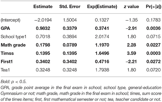
Table 3. Logistic regression with dataC and selected features (dataC select).
For the logistic regression with elastic net regularization we analyze one model with pure lasso/L1 (α = 1) regularization, two mixed models with α = 0.6 and α = 0.3 and one model with pure ridge/L2 (α = 0) regularization. The best results are found for the model with α = 0.3 thus we proceed with this model.
Table 4 shows the resulting feature ranking and the selected subset for both SVM methods, obtained by and their respective algorithms. Note that the ranking only marks the feature that is removed for the next subset. This evaluation is done within each subset. Rankings within the selected subsets are meaningless, except for the last ranked feature, which is chosen to be removed in the next step. This means in the best selected subsets the feature “school type” is marked as the least important feature. There is no ranking within this subset for the remaining features. In addition to the “school type,” the best subset consists of the “math grade,” “GPA,” “timss,” “tea,” and “first.” As a comparison, the loo.cv for the complete model (which has not been selected) is reported as well. The selected subsets for both methods are identical.
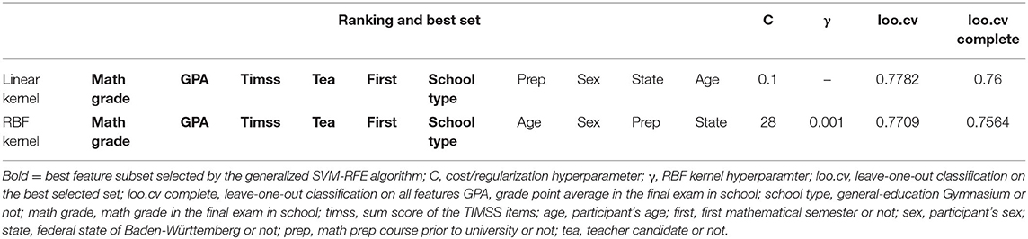
Table 4. Linear and generalized SVM-RFE for linear and RBF kernel: ranking and selected subsets for dataC.
The conditional inference tree uses the often selected features “math grade,” “GPA,” “timss,” and “tea” to do the splits. The specific splits are shown in Figure 1. Note that even though node 7 executes a further split, when used as a predictor the decision tree predicts a failure for all participants in the two terminal nodes 8 and 9, because of pass frequencies lower than 0.5.
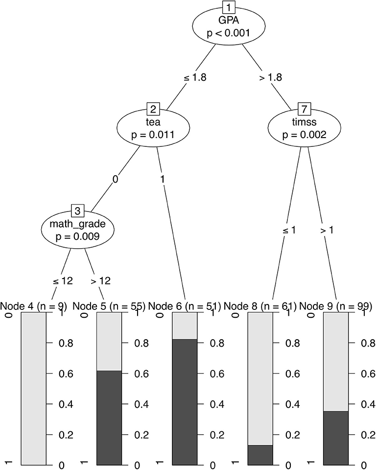
Figure 1. Conditional inference tree with the selected features and splits. The figure shows the split-points within the features used for splits. In the terminal nodes 4–6, 8, 9 the frequencies of the target variable “pass” is shown. GPA, grade point average in the final exam in school; tea, teacher candidate or not; timss, sum score of the TIMSS items; math_grade, math grade in the final exam in school.
For the conditional forest, the value of the number of features randomly selected in each split (mtry) is set via cross-validation to mtry= 2 (default value is mtry= 5). Feature selection depends on variable importance. Here we can see a slight dependence on the random seed. Those dependencies only occur within the second and third to last ranked features “state” and “prep.” Conditional variable importance is calculated three times with different random seeds. In Table 5 the sorted, absolute values of the means are reported. Even though there is no clear cut in feature importance, consistent to the other methods, we select the ranked features “school type” to “math grade” and compare the model with these features to the complete model. We choose this cut to compare the results with the SVM, where the same subset has been selected.
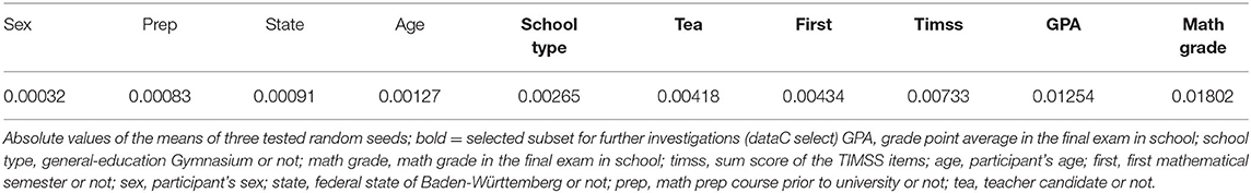
Table 5. Sorted list of the conditional variable importance for the conditional forest and the feature selection used in further analysis.
The best feature subsets for the methods are summarized in Table 6. Except for the single conditional inference tree, all of the most successful algorithms selected the same feature subset. This is remarkable, because the feature selection is done for each algorithm separately and with algorithm specific, appropriate methods. In addition to the performance measures (“GPA,” “math grade,” and “timss”), the school type (“school type”), first mathematical semester or not (“first”) and the major (“tea”) is selected. For the predictions, the major (“tea”) is selected as feature, even though this is the only selected variable that shows no significant result in the coefficients of the logistic regressions.
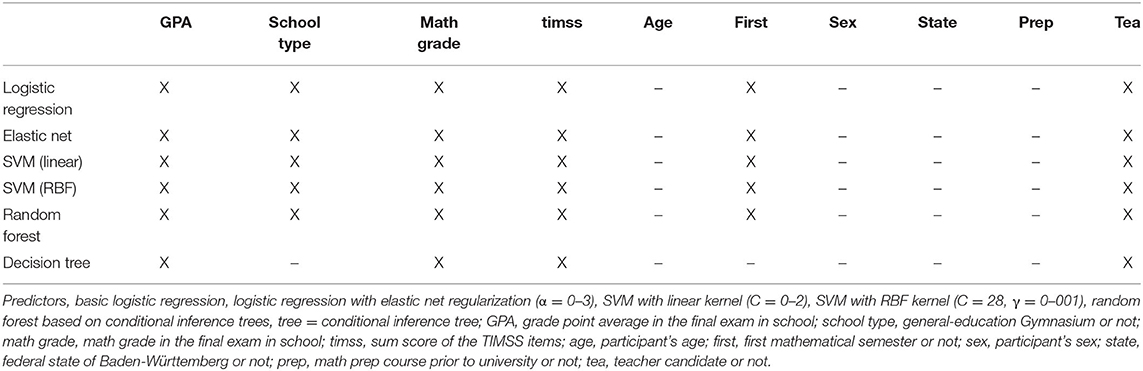
Table 6. Selected features for the different methods.
Prediction Comparison and Ensemble of the Predictors
In this section, we summarize the above-mentioned models. With all the selected models, we predict the target “pass.” To compare the predicted outcomes of the different models we calculate the inter-rater agreement between the models. Tables for those κ-values are presented in Table 7 for Cohen's Kappa on the training set and on the test set.
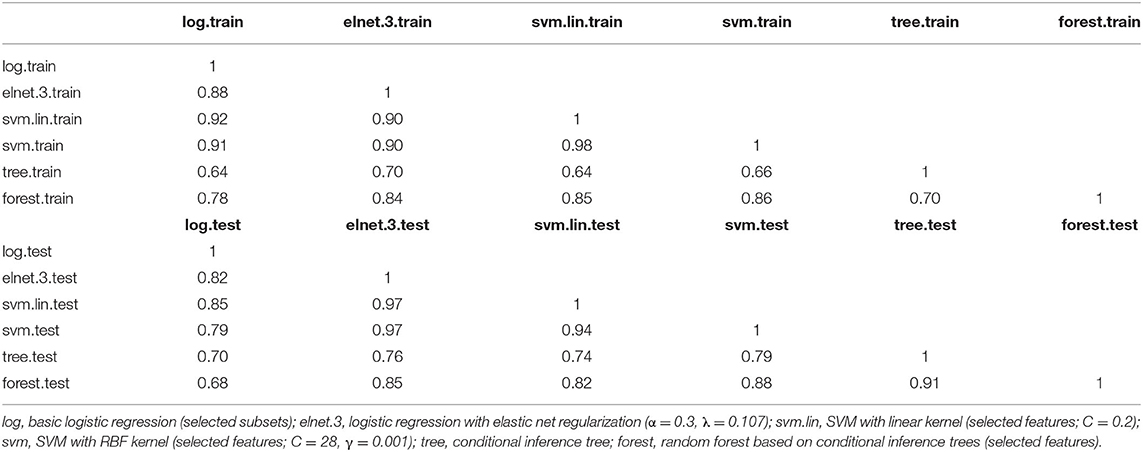
Table 7. Table of inter-rater agreement (κ) for the different best predictors on the training set and on the test set.
On both the training set and the test set, the different algorithms show at least substantial and often almost perfect inter-rater agreement.
We use all the predictors to build an ensemble predictor. In the ensemble, a majority vote is used to gain the overall prediction. In Table 8 the prediction measures for this ensemble and the single predictors are reported.
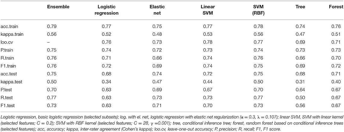
Table 8. Summary of the prediction measures of the best predictors.
For the two logistic regression approaches we can see better generalization results for the method with elastic net regularization. The high variance (overfitting) problem of the basic logistic regression can also be seen in the κ-values, which drop from moderate agreement on the training set (0.52) to fair agreement (0.34) on the test set. The SVM models show moderate inter-rater agreement on the test set. The models show slightly more overfitting than the logistic regression with elastic net regularization but result in the comparable test accuracy of 0.75 for the RBF kernel. As expected, the SVM with the RBF kernel outperforms the linear SVM. The single conditional inference tree shows overfitting, resulting in a total test accuracy of 0.68 and only fair inter-rater agreement (κ = 0.31). Both SVM algorithms, the logistic regression with elastic net regularization and the random forest achieve test accuracies higher than 0.70 and moderate inter-rater agreement. The two outstanding algorithms are the logistic regression with elastic net regularization (α = 0.3) and the SVM with RBF kernel. Both achieve the highest test accuracy (0.74 and 0.75, respectively) as well as the highest inter-rater agreement kappa test (0.47 and 0.50, respectively). The ensemble predictor does not outperform the best single predictors. This is no surprise, due to the high inter-rater agreements shown in Table 7. It more or less adopts the prediction measures of the SVM with RBF kernel and the logistic regression with elastic net regularization (α = 0.3).
Identification and Description of the Risk Group (R3)
For the identification of the different prediction groups (true positive predictions, true negative predictions and wrong predictions), we use the ensemble predictor to gain predictions for the complete dataset. This dataset contains the training set and the test set, which results in accuracy measures (Table 9) different to those reported in Table 8 (closer to the training measures due to the distribution in the train-test split).
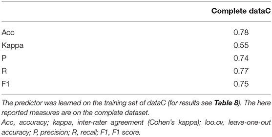
Table 9. Prediction measures of the ensemble predictor.
In Table 10 descriptive measures of the three groups are given. The performance measures from school—GPA and math grade—, as well as the test performance on the TIMSS items show the relation of performance and success. With regard to the ranges of the performance measures, we can see that for students with a GPA worse than 2.4 and a math grade worse than 9 points the success is not once correctly predicted. For students with a GPA better than 1.3 no correct failure prediction occurs. The ranges of the wrong predictions are rather wide. This could stress the importance of the behavior during the semester, as fortunate prerequisites don't necessarily lead to success and unfortunate prerequisites don't necessarily lead to failure. The descriptive measures in Table 10 only give general information on the groups but no indication on the structure or interaction of the features, which lead to different group assignments.
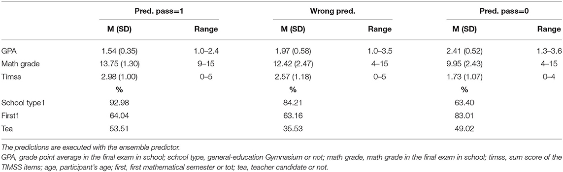
Table 10. Descriptive measures of the groups with correct positive prediction, correct negative prediction and wrong predictions on the complete dataset dataC.
For different applications, we partition the feature space using a conditional inference tree and assign terminal nodes to the risk group. Results of the decision tree are shown in Figure 2.

Figure 2. Conditional inference tree for the group membership of correct positive predictions, correct negative predictions and wrong predictions. The figure shows the split-points within the features used for splits. In the terminal nodes 4, 5, 7, 8, 11, 12, 14, and 15 the frequencies of the group membership are shown, with group 0 being the true negative predictions, group 1 the true positive predictions and group 2 the wrong predictions. The risk group is defined as the true negative predictions. The terminal nodes 4, 5, 8, and 14 are assigned to this group. Predicted outcomes of the ensemble predictor for the complete dataset dataC are used. GPA, grade point average in the final exam in school; school type, general-education Gymnasium or not; timss, sum score of the TIMSS items; math_grade, math grade in the final exam in school; first, first mathematical semester or not.
Figure 2 shows eight terminal nodes. We assign nodes 4, 5, 8, and 14 to the risk groups, because in those nodes the frequency of true negative predictions is outstandingly high compared to the rest. The first split is done at a math grade under and above of 12 points. In the following we describe some of the paths.
The ensemble predictor is especially confident about the failure of the students in node 4 and node 5. Those nodes contain students in their first mathematical semester, with a math grade in the final exam in school below or equal to 12 points. For students that are not in their first mathematical semester, a further split is executed at a GPA of 2.1, with GPAs worse than 2.1 leading to terminal node 8, which also is assigned to the risk group.
Students with math grades better than 12 points, are also allocated by their GPA. For students with a GPA worse than 1.6 the math performance is re-assessed with the TIMSS items. Students with 2 correct answers or less are assigned to terminal node 14 and thus to the risk group. Another interesting result shown in Figure 2 is the relevance of the school type. According to the results, the success in the Analysis 1 lecture for students with good school grades (more than 12 points in the final math exam and a GPA better than 1.6) highly depends on the school type. If the grades are achieved at a general-education Gymnasium, the prediction of success is very confident. For other school types the frequency of positive predictions is still the highest, but by far not as confident. This shows that in this analysis the value of school grades highly depends on the school type.
In summary, there are three paths leading to the risk group, which suggest three especially unfortunate prerequisite constellations. We will summarize these constellations in three risk levels, with the highest risk in risk level one. Students assigned to risk level one have 12 points or below in the final math exam and a GPA higher than 2.1. Risk level two is defined by math grades of 12 points or below and a GPA better than 2.1. Those students might have problems completing the Analysis 1 lectures in the first semester. The risk level three contains students with good math grades (above 12 points) but GPAs not better than 1.6. As already mentioned, the math performance is re-assessed with TIMSS items for this group−2 or less correctly answered items lead to as risk. The risk levels are summarized in Table 11.
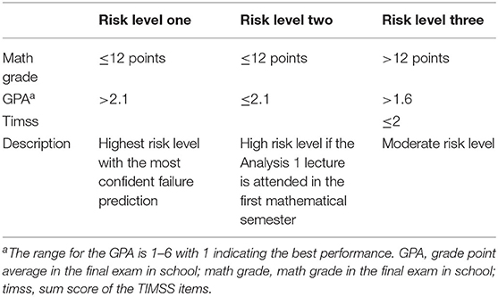
Table 11. Description of three risk levels with especially unfortunate prerequisites.
Discussion
With regard to the three research questions, the discussion is structured as follows. First, we review the results of students' different prerequisites prior to university (R1). We primarily focus on the teacher candidates and their possible differences with other mathematics students. Secondly, we discuss the most predictive features found by the different methods together with the achieved accuracies (R2) and thirdly, we discuss the described risk groups (R3).
Differences in Prerequisites of Teacher Candidates (R1)
We compared the prerequisites of B.Ed. students with those of B.Sc. students4. For the GPA, we can reproduce the result of Klusmann et al. (2009), showing no differences for the two groups. Thus, a negative selection concerning the general performance in school is not existent in the data. Other than their results, there are differences in the math specific performance measures “math grade” and “timss,” where the B.Sc. students performed better. This might be due to the different sample used in this study and in Klusmann et al. (2009). We compare teacher candidates in math with B.Sc. students in math and physics, whereas Klusmann et al. (2009) uses the TOSCA data set (Köller et al., 2004), where B.Sc. students with scientific subjects, also outside of the math and physics field are included as well. This means that the different results might occur because of a substantial positive selection in our B.Sc. group. The group differences regarding participation in a mathematical prep course prior to university, with only 20% of the B.Ed. students compared to 50% of the B.Sc. students, need further investigation. The University of Tübingen offers mathematical prep courses for physics and computer science, but no course specifically designed for math students. Even though those courses are open to math students as well, they might be more present in the physics study recommendations, thus the physics students within the B.Sc. group might cause the above-mentioned difference. In the framework of this study, the difference of the variable “first” needs to be discussed. Only 58% of the B.Ed. students were in their first mathematical semester, compared to 86% of the B.Sc. students. The data doesn't contain the information if the students, who are not in their first mathematical semester, already participated in an Analysis 1 lecture before, or if, for example, they attended lectures in linear algebra first. Due to the study design, we can eliminate partly successful participations in former Analysis 1 lectures. It is a possible scenario for B.Ed. students not to start with the analysis and linear algebra lectures simultaneously, which would be the common way especially for the B.Sc. students. This has an influence on the non-completions in this data as seen in the importance of the feature “first” in the predictions and feature selections. This might be due to general experience gained at university, even though the lecture itself is attended for the first time. For that reason, it was important to include the feature “first” to capture this effect when evaluating the group of teacher candidates.
Identification of the Most Predictive Features and Prediction Accuracies (R2)
For the identification of the most predictive features, method specific algorithms are used. All of the best predictors (excluding the single decision tree) use the same feature subset, including grade point average of the final exam in school (“GPA”), the information if the school type where the final exam is done was a general-education Gymnasium (“school type”), the math grade in the final exam in school (“math grade”), the sum score of the TIMSS items (“timss”), the information if the students were in their first mathematical semester (“first”) and if the students are in the B.Ed. (teacher candidates) or in the B.Sc. study program (“tea”).
As expected, the math specific performance measures and the general school performance measure show positive effects on the success in the Analysis 1 lecture (see e.g., Bean, 2005). As mentioned earlier, there is a positive effect concerning students' number of mathematical semester. Students which are not in their first mathematical semester show higher success probabilities than students in their first semester. This effect was expected, because even though the students might not have participated in a former Analysis 1 lecture, they don't have to deal with general problems at the beginning of university and might be more experienced in handling the requirements of a math lecture. Even though in the basic logistic regression being a teacher candidate shows no significant coefficient for the dependent variable indicating the success in Analysis 1, in prediction, all methods selected “tea” as a predictive feature. Over all, we see slight indication of a positive effect of “tea” on the success. For example, the single decision tree selects “tea” as one of the splitting features with a positive effect. This might be due to the high frequency of students not in their first semester within the teacher candidates. Since the feature “first” is not selected by the tree, its positive effect might occur within the feature “tea.”
Students who graduated at a general-education Gymnasium are more likely to pass the Analysis 1 lecture. This influence of the school type can only be discussed speculatively, because the data doesn't reveal further information. In some of the alternative school types, the students attend a lower level school first and then transfer to a school were the admission to a university can be achieved. Those differences, for example in the math knowledge, might not be seen in the restricted framework of the final exams in school, but seems to have an influence on success probabilities at the university.
Except for the basic logistic regression and the single conditional inference tree, the best predictors of the respective methods all achieve accuracies on the test set above 70%. The F1-scores are in a good range between 0.6 and 0.73 for all predictors (except for the single tree) and show no substantial tradeoff between recall and precision, indicating, as expected, no serious effect of the slightly skewed data.
As a result, we summarize that with appropriate methods the success in the Analysis 1 lecture can be correctly predicted for 75% of the students (with inter-rater agreement in the moderate range), only with the knowledge of their GPA, their math grade in the final exam in school, the test result of the TIMSS items, the school type and their number of semesters and study program. Note that this is the accuracy on the test set meaning after possible generalization errors.
Risk Groups
The results of this study can help universities to identify risk groups in math study programs. Here we see that unfortunate performance measures from school lead to the expected risk of a failure in Analysis 1. The results underline the results of previous studies (see e.g., Bean, 2005), but furthermore give thresholds for the math grade of 12 points and a school GPA of 2.1. We also see that a good mathematical performance in school (>12 points) needs to be confirmed by additional mathematical performance tests, like the TIMSS items (at least as long as the GPA is not in the excellent range, here >1.6). Note, that even though we need six variables for accurate predictions, the risk level identification can be done by using at most three variables. Investigations that lead to resilient risk group classifications lead to different easy-to-use recommendations. First, if necessary, an admission restriction can be applied for students with risk level one (math grade worse or equal to 12 points and GPA worse than 2.1). Secondly, interventions like mathematics pre-courses can be offered before the semester begins, in particular for students in the risk levels. And thirdly, interventions during the semester, such as mentoring programs or support lectures, can be planned and offered for the target group of students with high risk levels.
Conclusion
We conclude that teacher candidates start with adverse prerequisites concerning math specific performance measures. However, there are no significant differences to B.Sc. students in terms of success in the Analysis 1 lecture. Success in the Analysis 1 depends on the number of the mathematical semesters with a positive effect of not being in the first semester. The distribution of this variable within the teacher candidates might contribute to a slight overall positive effect of being a teacher candidate. The analysis of the risk groups also indicates the disagreement with the public opinion of teacher candidates being the worse students, described in Blömeke (2005). The study program itself does not occur as indicator for a risk group. But one should mention that a threshold for the math grade in school can be set at 12 points (see previous section). The B.Ed. students however show significantly worse math grades compared to their B.Sc. colleagues (11.43 and 12.06, respectively) with the mean lying slightly below the threshold. An assumable negative effect on the success however did not occur in our analysis and although the teacher candidates show worse prerequisites in math performance the school grades are still in the good range. In conclusion, we say that, at least in our dataset, the teacher candidates show no substantially disadvantageous prerequisites for the success in the Analysis 1 lecture and thus do not represent a risk group per se [(R1) and (R3)].
With regard to the variable clusters of Bean (2005) and Burrus et al. (2013), the analysis did not show effects in the field of students' demographic characteristics, age and sex, but in the high relevance of the academic preparation and success factors. The indication of risk groups highly depends on performance measures from school or at least on their underlying concepts of knowledge. We saw that the school grades in some cases have to be confirmed by additional tests or the knowledge about the school types where the grades were achieved. Due to the limitations of the study, clear recommendations for interventions have to be made carefully. In general, this procedure can lead to the resilient identification of risk group indicators and the classification of the risk levels, which can be extremely helpful for universities when discussing admission restrictions. Table 11 shows the highest risk for students with school grades below average (math grades of ≤ 12 points and GPAs higher than 2.1). Especially the math grade seems to be a good indicator for students in risk groups. With meaningful risk group classifications, other applications apart from admission restrictions can be the development of interventions and general support courses for specific target groups. Even though the results might not give suggestions for specific variables which could be improved by interventions, it helps to identify risk groups for which interventions or support courses should be developed. For this task Figure 2 can be used.
This analysis relies on results of the ensemble predictor, which shows a test accuracy of 75%. This accuracy is only achieved using a small set of features, consisting of information prior to the lecture (R2). Considering that no information about students' behavior during the semester is included, this is a rather high value. Note that the accuracy refers to predictions on the test set, consisting of students the algorithm has never seen bevor. The remaining 25% of the students show wide ranges of variable values. Again, this stresses the importance of the behavior during the semester. On the one hand, even students with very unfortunate prerequisites can succeed in the lecture and, on the other hand, very fortunate prerequisites don't guarantee the success. With the high accuracy of 75%, a general structure seems to be found, resulting, for example, in the identification of risk groups.
The methods were applied in the German setting of teacher education. Due to differences for example to the U.S. system, results and conclusions might not directly be applicable. But the general procedure can be adopted and suggests the use of data science methods to improve teacher education. For example, in the U.S. the SAT-/ACT-scores might be included.
Limitation and Outlook
In this study, data of two consecutive Analysis 1 lectures at the University of Tübingen was used. Even though, instead of sampling, all students of the lecture were included (with a return rate around 92%), the data might only be representative for this university. Especially concerning the federal state, where 87% of the participants graduated at a school in the state of Baden-Württemberg, the data might not be representative for Germany. With the combination of two lectures we tried to address the possible dependence on lecturers and specific schedules. For further improvement the inclusion of more lectures, in particular lectures at different universities, would be appropriate. Concerning the used variables, one should consider aspects concerning students' personality and motivation.
Due to sample size and the limitation implied by only considering one university, specific results have to be interpreted very carefully. Even though the course used is thought to be representative for the initial phase of mathematics study programs, different educational systems might influence the success enormously. Thus, specific results, like variable selection and thresholds in risk classification, might not generalize well in other contexts. Nevertheless, the applied methods and the general procedure can be generalized and provide valuable information when applied by educational institutions.
As mentioned before this study serves as an example of the usefulness of data science methods in teacher education, especially when the focus is on applicability where algorithms have to deal with sparse feature spaces.
As next steps, the inclusion of behavioral information during the semester is planned, including a wider range of students' characteristics. For a better generalization, more universities in Baden Württemberg will be included.
Although, this study is a very specific perspective on student drop out, given the German education system, we feel that the general procedure has its merits in terms of risk identification and potential for interventions.
Data Availability Statement
The datasets generated for this study will not be made publicly available. The informed written consent permits the use of the data and the publication of results but not the publication of datasets.
Ethics Statement
Ethical review and approval was not required for the study on human participants in accordance with the local legislation and institutional requirements. The patients/participants provided their written informed consent to participate in this study.
Author Contributions
The main research was undertaken by PK with consultation by FL regarding mathematical topics and AK regarding statistical topics. The manuscript was written by PK with editing help of FL and AK. All authors contributed to the article and approved the submitted version.
Funding
This project is part of the Qualitäts offensive Lehrerbildung, a joint initiative of the Federal Government and the Länder which aims to improve the quality of teacher training. The programme was funded by the Federal Ministry of Education and Research. The authors are responsible for the content of this publication. This work was funded by the Deutsche Forschungsgemeinschaft (DFG, German Research Foundation) under Germany's Excellence Strategy - EXC number 2064/1 - Project number 390727645.
Conflict of Interest
The authors declare that the research was conducted in the absence of any commercial or financial relationships that could be construed as a potential conflict of interest.
Acknowledgments
The main findings of this manuscript arise from the doctoral thesis (Kilian, 2018).
Supplementary Material
The Supplementary Material for this article can be found online at: https://www.frontiersin.org/articles/10.3389/feduc.2020.502698/full#supplementary-material
Footnotes
1. ^K4, K5, K6, L5, L6 of TIMSS/III, Rasch scaled.
2. ^Comparable with the U.S. cumulative/overall High School GPA.
3. ^In machine learning literature the dependent variable is often referred to as target (variable).
4. ^The analysis for the performance measures “GPA,” “math grade,” and “timss” was repeated and con- trolled for sex. The results did not change and thus are not reported.
References
Adams, R. J., Wu, M. L., and Macaskill, G. (1997). Scaling methodology and procedures for the mathematics and science scales. TIMSS Tech. Rep. 2, 111–145.
Alyahyan, E., and Düştegör, D. (2020). Predicting academic success in higher education: literature review and best practices. Int. J. Educ. Technol. Higher Educ. 17. doi: 10.1186/s41239-020-0177-7
Baumert, J., Bos, W., Klieme, E., Lehmann, R., Lehrke, M., Hosenfeld, I. (eds.). (1999). Testaufgaben zu TIMSS/III: Mathematisch-naturwissenschaftliche Grundbildung und voruniversitäre Mathematik und Physik der Abschlussklassen der Sekundarstufe II (Population 3), Vol. 62. Berlin: Max-Planck-Institut für Bildungsforschung.
Bean, J. P. (1980). Dropouts and turnover: The synthesis and test of a causal model of student attrition. Res. Higher Educ. 12, 155–187. doi: 10.1007/BF00976194
Bean, J. P. (1983). The application of a model of turnover in work organizations to the student attrition process. Rev. Higher Educ. 6, 129–148. doi: 10.1353/rhe.1983.0026
Bean, J. P. (2005). “Nine themes of college student retention,” in College Student Retention: Formula for Student Success, ed A. Seidman (New York, NY: Rowman and Littlefield), 215–244.
Berens, J., Schneider, K., Gortz, S., Oster, S., and Burghoff, J. (2019). Early detection of students at risk - predicting student dropouts using administrative student data from German Universities and Machine Learning Methods. J. Educ. Data Mining 11, 1–41. doi: 10.5281/zenodo.3594771
Burrus, J., Elliott, D., Brenneman, M., Markle, R., Carney, L., Moore, G., et al. (2013). Putting and Keeping Students on Track: Toward a Comprehensive Model of College Persistence and Goal Attainment. ETS Research Report Series. Wiley. doi: 10.1002/j.2333-8504.2013.tb02321.x
Chen, X. (2013). STEM Attrition: College students' paths into and out of STEM fields (NCES 2014-001). Washington, DC: National Center for Education Statistics, Institute of Education Sciences, U.S. Department of Education.
Cohen, J. (1960). A coefficient of agreement for nominal scales. Educ. Psychol. Meas. 20, 37–46. doi: 10.1177/001316446002000104
Eilerts, K. (2009). Kompetenzorientierung in der Mathematik-Lehrerausbildung: empirische Untersuchung zu ihrer Implementierung, Vol. 14. Münster: LIT Verlag.
Evgeniou, T., Pontil, M., and Elisseeff, A. (2004). Leave one out error, stability, and generalization of voting combinations of classifiers. Mach Learn. 55, 71–97. doi: 10.1023/B:MACH.0000019805.88351.60
Feldman, M. J. (1993). Factors associated with one-year retention in a community college. Res. Higher Educ. 34, 503–512. doi: 10.1007/BF00991857
Friedman, J., Hastie, T., and Tibshirani, R. (2010). Regularization paths for generalized linear models via coordinate descent. J. Stat. Softw. 33, 1–22. doi: 10.18637/jss.v033.i01
Grünwald, N., Kossow, A., Sauerbier, G., and Klymchuk, S. (2004). Der Übergang von der Schul- zur Hochschulmathematik: Erfahrungen aus internationaler und deutscher Sicht. Global J. Eng. Educ. 8, 283–293.
Gueudet, G. (2008). Investigating the secondary–tertiary transition. Educ. Stud. Math. 67, 237–254. doi: 10.1007/s10649-007-9100-6
Guyon, I., Weston, J., Barnhill, S., and Vapnik, V. (2002). Gene selection for cancer classification using support vector machines. Mach. Learn. 46, 389–422. doi: 10.1023/A:1012487302797
Hagedorn, L. S., Maxwell, W., and Hampton, P. (2001). Correlates of retention for african-american males in community colleges. J. Coll. Stud. Retent. Res. Theory Pract. 3, 243–263. doi: 10.2190/MJ6A-TFAC-MRPG-XDKL
Hastie, T., Tibshirani, R., and Friedman, J. (2009). The Elements of Statistical Learning: Data Mining, Inference, and Prediction, 2nd Edn. New York, NY: Springer.
Heublein, U. (2014). Student dropout from german higher education institutions. Eur. J. Educ. 49, 497–513. doi: 10.1111/ejed.12097
Heublein, U., Hutzsch, C., Schreiber, J., Sommer, D., and Besuch, G. (2009). Ursachen des Studienabbruchs in Bachelor- und in herkömmlichen Studiengängen: Ergebnisse einer bundesweiten Befragung von Exmatrikulierten des Studienjahres 2007/08. Hannover: HIS Hochschul-Informations-System.
Holland, J. L. (1997). Making Vocational Choices: A Theory of Vocational Personalities and Work Environments, 3rd Edn. Odessa, FL: Psychological Assessment Resources.
Hothorn, T., Buehlmann, P., Dudoit, S., Molinaro, A., and Van Der Laan, M. (2006a). Survival ensembles. Biostatistics 7, 355–373. doi: 10.1093/biostatistics/kxj011
Hothorn, T., Hornik, K., and Zeileis, A. (2006b). Unbiased recursive partitioning: a conditional inference framework. J. Comput. Graph. Stat. 15, 651–674. doi: 10.1198/106186006X133933
Kilian, P. (2018). On Ck, PCK and Student Dropout in the Early Phase of Math (Teacher) Education at University (Doctorial thesis). University of Tübingen, Germany.
Klusmann, U., Trautwein, U., Lüdtke, O., Kunter, M., and Baumert, J. (2009). Eingangsvoraussetzungen beim Studienbeginn: Werden die Lehramtskandidaten unterschätzt? Zeitschrift Pädagogische Psychol. 23, 265–278. doi: 10.1024/1010-0652.23.34.265
Köller, O., Watermann, R., Trautwein, U., and Lüdtke, O. (eds.). (2004). Wege zur Hochschulreife in Baden Württemberg. TOSCA – Eine Untersuchung an Allgemeinallgemein und Beruflichen Gymnasien. Opladen: Leske + Budrich.
Kunter, M., Baumert, J., Blum, W., Klusmann, U., Krauss, S., and Neubrand, M. (eds.). (2011). Professionelle Kompetenz von Lehrkräften: Ergebnisse des Forschungsprogramms COACTIV. Waxman Gmbh.
Landis, J. R., and Koch, G. G. (1977). The measurement of observer agreement for categorical data. Biometrics 33, 159–174. doi: 10.2307/2529310
Leppel, K. (2002). Similarities and differences in the college persistence of men and women. Rev. Higher Educ. 25, 433–450. doi: 10.1353/rhe.2002.0021
Meyer, D., Dimitriadou, E., Hornik, K., Weingessel, A., and Leisch, F. (2017). e1071: Misc Functions of the Department of Statistics, Probability Theory Group (Formerly: E1071), TU Wien [Computer Software Manual]. (R package version 1.6–8) Wien: TU Wien.
Mullis, I. V., Martin, M. O., Ruddock, G. J., O'Sullivan, C. Y., Arora, A., and Erberber, E. (2007). TIMSS 2007 Assessment Frameworks. Boston, MA: Lynch School of Education, Boston College, TIMSS and PIRLS International Study Center.
Nagy, G. (2007). Berufliche Interessen, kognitive und fachgebundene Kompetenzen: Ihre Bedeutung für die Studienfachwahl und die Bewährung im Studium (Ph.D. thesis). Freie Universität, Berlin. Retrieved from: https://www.fachportal-paedagogik.de/literatur/vollanzeige.html?FId=847822#vollanzeige (accessed November 10, 2020).
Pérez, B., Castellanos, C., and Correal, D. (2018). Predicting Student Drop-Out Rates Using Data Mining Techniques: A Case Study. Cham: Springer, 111–125.
R Core Team (2015). R: A Language and Environment for Statistical Computing [Computer software manual]. Vienna: R Core Team.
Rakotomamonjy, A. (2003). Variable selection using svm based criteria. J. Mach. Learn. Res. 3, 1357–1370.
Schiefele, U., Streblow, L., and Brinkmann, J. (2007). Aussteigen oder Durchhalten. Was unterscheidet Studienabbrecher von anderen Studierenden? Zeitschrift Entwicklungspsychol Pädagogische Psychol. 39, 127–140. doi: 10.1026/0049-8637.39.3.127
Strobl, C., Boulesteix, A.-L., Kneib, T., Augustin, T., and Zeileis, A. (2008). Conditional variable importance for random forests. BMC Bioinform. 9:307. doi: 10.1186/1471-2105-9-307
Strobl, C., Boulesteix, A.-L., Zeileis, A., and Hothorn, T. (2007). Bias in random forest variable importance measures: Illustrations, sources and a solution. BMC Bioinform. 8:25. doi: 10.1186/1471-2105-8-25
Terenzini, P. T., and Pascarella, E. T. (1980). Toward the validation of tinto's model of college student attrition: a review of recent studies. Res. Higher Educ. 12, 271–282. doi: 10.1007/BF00976097
Tinto, V. (1975). Dropout from higher education: a theoretical synthesis of recent research. Rev. Educ. Res. 45, 89–125. doi: 10.3102/00346543045001089
Tinto, V. (1987). Leaving College: Rethinking the Causes and Cures of Student Attrition. Chicago, IL: University of Chicago Press.
Keywords: student retention, mathematics, math teacher training, higher education, machine learning, dropout prediction
Citation: Kilian P, Loose F and Kelava A (2020) Predicting Math Student Success in the Initial Phase of College With Sparse Information Using Approaches From Statistical Learning. Front. Educ. 5:502698. doi: 10.3389/feduc.2020.502698
Received: 04 October 2019; Accepted: 04 November 2020;
Published: 22 December 2020.
Edited by:
Ida Ah Chee Mok, The University of Hong Kong, Hong KongReviewed by:
Wang Ruilin, Capital Normal University, ChinaKerstin Schneider, University of Wuppertal, Germany
Copyright © 2020 Kilian, Loose and Kelava. This is an open-access article distributed under the terms of the Creative Commons Attribution License (CC BY). The use, distribution or reproduction in other forums is permitted, provided the original author(s) and the copyright owner(s) are credited and that the original publication in this journal is cited, in accordance with accepted academic practice. No use, distribution or reproduction is permitted which does not comply with these terms.
*Correspondence: Pascal Kilian, cGFzY2FsLmtpbGlhbkB1bmktdHVlYmluZ2VuLmRl