Grid-Aware Layout of Photovoltaic Panels in Sustainable Building Energy Systems

Introduction

Today, it is widely accepted that climate change is a threat to both human and natural ecosystems, and that the increasing greenhouse gas emissions from anthropogenic activities are at the root of the warming of the climate (Pachauri et al., 2014).

Among all human-related activity sectors, buildings accounted for 36% of the global final energy use and 39% of the greenhouse gas emissions in 2018 (Global Alliance for Buildings and Construction, International Energy Agency and the United Nations Environment Programme, 2019). Among the latter, residential buildings globally accounted for 61% of the final energy use and 41% of the emissions. Furthermore, over 50% of the global final energy use in residential buildings is related to space and water heating (Lucon et al., 2014; Global Alliance for Buildings and Construction, International Energy Agency and the United Nations Environment Programme, 2019).

To decrease carbon emissions, several solutions have been suggested to increase carbon efficiency while fulfilling heating requirements for residential buildings. Whereas several researchers have focused on reducing the demand, another solution is to move away from high-carbon fossil fuels, thereby switching from natural gas and oil to low carbon fuels such as green electricity. In particular, switching to electrical HVAC systems allows a higher conversion efficiency and improves the integration of locally generated renewable energy, such as by installing photovoltaic (PV) panels on rooftops (Lucon et al., 2014; Pachauri et al., 2014). However, volatile power generation caused by the fluctuation of solar irradiation challenges the capacity of the electrical power grid. Therefore, in addition to maximizing the energy generated from the Sun, it is important to reduce the interaction of the building energy system (BES) with the electrical power grid by maximizing self-consumption while decreasing the grid’s energy demand.

Multi-Objective Optimization Framework of Building Energy Systems

The vast number of alternative solutions availible to reduce the carbon footprint of BES makes the choice of the appropriate system a complex decision. For this reason, several studies dealing with energy system optimization have focused on it. In particular, when renewable energy generation is involved, the target is to identify economical and environmental friendly solutions for BESs that cover thermal and electricity demand while protecting the grid and therewith secure the supply.

Consequently, many similar BES optimization problems exist and are generally characterized by having multiple, competing objectives. The most common include capital expenses (CAPEX), operational expenses (OPEX), and global warming potential (GWP). This forces researchers to adopt a multi-objective optimization (MOO) approach. The MOO of BES has been the focus of extensive research over the past years (Jennings et al., 2014; Stadler et al., 2014; Rager, 2015; Morvaj et al., 2016; Wu et al., 2017; Jing et al., 2018; Ma et al., 2018; Stadler et al., 2018; Stadler, 2019).

Within the framework of BES optimization, many models have included PV panels as one alternative for distributed energy generation. In most cases, the electricity generated by PV panels has been modeled by an efficiency converting solar radiation to electricity. Because of the need to reduce model complexity, these models are generally relatively simple. It is common to use the total irradiation, often referred to as global irradiation, to model the incoming solar radiation, which corresponds to assuming horizontal panels (Duffie and Beckman, 2013).

In general, studies focusing on the energy system have not accounted for varied panel orientation, and only the most detailed PV models have included the influence of different ambient conditions (such as external temperature) on the efficiency of the conversion (Ashouri, 2014; Jing et al., 2018; Ma et al., 2018) or on panel degradation (Fan and Xia, 2017).

A detailed literature review has revealed no prior investigation on the role of the incident angle of solar irradiation on PV panels, with the exception of thermal solar panels, where the roof orientation was set as the orientation of the thermal solar panel (Rager, 2015).

Simulation and Optimization of Solar Based Energy Systems

The increasing penetration of solar energy in the electricity network has confronted the grid operators with new challenges. The demand during solar noon hours is decreasing, whereas the demand after sunset is increasing, causing a sharp ramp in evening hours. Within this context, adapting the supply to match demand has become a compelling task (Lazar, 2016).

Research in the field of solar-based energy systems, however, has shown that panel/roof orientation and tilt have a substantial influence on the energy generation potential of PV panels, and that altering these variables can help to provide a better match between the demand and the energy availability from the PV modules. Thereby, researchers have focused on the optimal sizing of PV panels and batteries, maximizing objectives like the internal rate of return (Hartner and et, 2017) or minimizing costs (Holweger et al., 2019a).

van der Stelt et al. (2018) proposed a MILP framework to analyze PV–Battery system in techno-economical terms based on real demand and PV profiles with different orientations taken from smart meter measurements of 39 residential buildings in The The Netherlands. The authors demonstrated that although the increased self–consumption was the main contributor to annual saving, centralized and decentralized storage systems are economically infeasible. Unsurprisingly, high feed-in tariffs result in a larger optimal size for PV panels. Similarly, Holweger et al. (2019a) demonstrated the impact of different price signals on the optimal unit size and grid impact. Their optimization framework included storage and curtailment options but the orientation of the PV was fixed. Hartner etal. (2017) have not included storage or curtailment options and used a simulation tool to assess the electricity profiles generated by PV panels.

Varying the orientation of the PV modules allows for a better match between the demand and energy availability from the PV modules, thus resulting in higher self–consumption and, hence, higher revenues, without the need for batteries. The economic advantage of self–consuming the energy produced by the PV modules instead of selling it to the grid operator largely depends on country–specific attributes, such as price profiles and the amount of generated electricity (Mondol et al., 2007; Lahnaoui et al., 2017; Litjens et al., 2017). However, given the challenges of grid stability arising from a more widespread adoption of distributed electricity generation, most countries are reducing the compensation for feeding in energy to the grid to promote self-consumption and, hence, reduce strong demand variations.

Litjens et al. (2017) showed that self–consumption is highest at 212° azimuth and 26° tilt for residential buildings in The Netherlands. Similar results were obtained in the United Kingdom by Mondol et al. (2007) and by Lahnaoui et al. (2017), who concluded that west–oriented PV systems have a higher share of directly consumed electricity than east–oriented systems for residential demand patterns in Germany. On the other hand, the maximum electricity generation was achieved for south–oriented systems (approximately 180° azimuth) and with a tilt angle approximately 30°. Although these values can change based on the system location (latitude and weather patterns), similar results have been found by researchers in Austria (Hartner and et, 2017), The The Netherlands and the United Kingdom (Mondol et al., 2007; Litjens et al., 2017). A maximum variation of the optimal orientation of about 7° toward the west and higher tilt angles were identified due to weather influence (Litjens et al., 2017).

Not all researchers, however, have agreed with the result that slightly west-oriented panels are the most optimal configuration. A recent study by Laveyne et al. (2020) investigated the impact of the orientation of PV modules on the grid, including the effects on grid losses and PV curtailment. Their results identified that the optimal orientation is the one that maximizes the annual generated electricity (south, 35° tilt in Belgium). Although this high generation also causes the highest curtailment and grid losses, changing the orientation did not lead to more useful energy. The authors also found, however, that changing the tilt angle had a higher impact on the grid than on the generation and thus suggested to lower tilt angles for more constrained grids (Laveyne et al., 2020).

Other researchers have confirmed that, although it might not be the most economically convenient choice, it is possible to contribute to preserving grid stability by changing the orientation. Sadineni et al. (2012), referring to a case study in the United States, showed that the combination orientating the PV modules to the west and load scheduling of the cooling demand can reduce the peak by more than 60%, although the most economical orientation at flat price profiles remains south. These results were confirmed by Rhodes et al. (2014), who evaluated the optimal placement of PV panels at a national level in the United States. They found that orientating the PV panels toward the south led to the maximum energy generated. Differently from Sadineni et al. (2012), however, they also showed that shifting the orientation 20°–50°westwards increased the economic value of the generated PV electricity by 1–7%. A further increase in the tilt and in the westward orientation was also identified as the optimal “peak placement,” as the system produced 24% more energy during peak demand hours (Rhodes et al., 2014).

However, as the optimal integration of PV and battery systems is the was the focus in the aforementioned studies, historical measurements of the electric demand have been commonly applied or the remaining technologies and the renovation state of the building is fixed a priori, leading to predefined demand profiles from the buildings.

Modeling of Photovoltaic Panel Orientation and Directed Irradiation

As highlighted in the previous section, the positioning of the PV modules (orientation and tilt angle) can significantly impact the model design of how such systems perform once included in the BES. This highlights the need for including models accounting for these effects on the energy generation profile of a solar panel.

Accessing the orientation of solar irradiation is important for urban planners to find the best building concepts and designs and to evaluate the solar potential of surfaces. An overview of detailed models for determining solar incident values was provided by Hafez et al. (2017), who focused on the optimal tilt angle and on how it varies with the location and season. Starting from the assumption that orientation is considered as optimal when the received irradiation is maximal, Hafez et al. (2017) presented optimal tilt angles from case studies from all over the world.

Irradiation models are generally classified into two categories. Isotropic models assume a uniform intensity of diffuse radiation over the skydome, whereas anisotropic sky models do not. Different models have been proposed by Badescu (2008); Hafez et al. (2017); Duffie and Beckman (2013). It is unfortunately controversial whether isotropic or anistropic models are more accurate, and literature in the field shows conflicting results. In general, anisotropic models are more detailed and computationally intensive, but have been found more accurate by the majority of case studies (e.g., Khoo et al. (2014) and Chwieduk (2009)). However, others, such as (Shukla et al., 2015), concluded that isotropic models provide a higher degree of accuracy.

Focusing on solar orientation modeling in an urban context, Freitas et al. (2015) provided an overview of empirical and computational solar radiation models and concluded that numerical radiation algorithms connected with geographic information systems (GIS) tools represent the most appropriate trade-off between accuracy and computational time. The application of a GIS based approach to evaluate solar potential including topographic impact was demonstrated by Bremer et al. (2016) for a city in Austria, by Ko et al. (2015) for Taiwan and by Verso et al. (2015) for a city in Spain. However, Verso et al. (2015) did not model shading, as only the best roofs were considered for PV installation. Vulkan et al. (2018) developed an open source package in R to model shading effects on building surfaces in Israel and concluded that south oriented facades could contribute significantly to annual electricity generation. The handling of shading on rooftops has been identified to be one of the main distinction of different assessments of solar potential in Switzerland (Walch et al., 2019). Assouline et al. (2017) proposed an approach using machine learning to extrapolate missing data using a combination of support vector machines and GIS to access the annual potential of Switzerland. Their method to assess monthly mean values in a high spatial resolution is included in the Swiss national project to determine the solar potential and to provide guidelines to building owners (Klauser, 2016). Although these studies have the focus on different orientation of single roofs, the aspect of the connected energy system remains a minor focus.

Gaps and Contributions

Based on the aforementioned literature review, there exists a gap in the state-of-the-art at the intersection between 1) studies focusing on BES, which only include a very simplified representation of the energy generated by PV panels, and 2) studies focusing on the optimal placement of PV panels, which never include how this affects, and is affected by, the integration with other parts of the BES. This work therefore aims to investigate the following research questions:

What is an optimal placement of PV panels (orientation and tilt) from the perspective of the individual building and of the grid? How does it depend on problem parameters such as the load profile and the characteristics of the building?

What are the principles that should be adopted when choosing the placement of increasing quantities of PV panels on the roof of the building?

What is the magnitude of the error induced by the assumption of only horizontally installed PV panels in energy system planning models?

How are different policies for subsidizing the installation of PV panels impacting the “optimal” orientation?

Materials and Methods

In the following study, an optimization approach is adopted, where the types and sizes of the different components of the BES, and the size, azimuth and tilt of the PV modules, are considered as optimization variables.

To this end, a robust and flexible modeling framework able to take into account the BES, solar based energy systems, and the impact of solar irradiation in an urban context is required. The modeling framework applied in this paper is based on the BES modeling by Stadler (2019). Instead of integrating PV modules solely based on global irradiation, oriented irradiation is included using the cumulative sky approach (Robinson and Stone, 2004) in combination with its integration into urban context (Schüler, 2018). The optimization of BES requires a time horizon of several years and therefore is a computationally intense task. To overcome this issue, it is necessary to reduce the amount of input data and select typical operation periods using machine learning techniques (Fazlollahi et al., 2014).

The modeling framework and its components are described in Energy System Modeling Framework, and the optimization approach is presented in Problem Formulation. The specific focus of the oriented irradiation and shading effects between oriented modules is explained in Irradiation and Photovoltaic Panel Modeling. Input Data and Its Clustering provides additional details about the clustering of input data.

Energy System Modeling Framework

The BES modeling framework is illustrated in Figure 1.

FIGURE 1

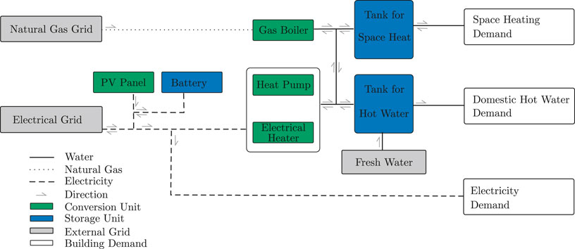
FIGURE 1. Building energy system structure (BES).

Three types of energy demands are considered: space heating (SH), domestic hot water (DHW), and electricity. The electricity demand is derived from measurements and further disaggregated using the method proposed by Holweger et al. (2019b); these uncontrollable load profiles are used as direct input to the model. The DHW demand is required to have a fixed supply temperature of at least 60°C. The average demand is estimated to 40 L per day and person, in case of residential buildings (SIA, 2015).

The space heating demand is impacted by factors such as the conductive heat losses through the building envelope, the heat capacity of the building, and the heat gains from occupants, electric appliances, and solar irradiation. Furthermore, space heating demand is characterized by the desired comfort temperature of the rooms and the nominal temperature of the heat distribution system (Girardin, 2012). This type of modeling of the energy demand allows, among others, for including the building temperature as a decision variable within a predefined comfort range, and hence use the building mass as a thermal energy storage. The building is considered to have access to two types of energy supply networks: the natural gas grid, and the electricity grid.

The BES modeling framework includes multiple unit technologies that can contribute to satisfy the different energy demands. Both the SH and DHW demands can be fulfilled by a gas boiler, converting natural gas into thermal energy, or by heat pumps and electrical heaters, both converting electricity to thermal energy. PV panels are also considered as energy conversion units, converting incoming solar irradiation to electricity. The system also includes storage technologies. Two different tanks are considered, one for SH and one for DHW, as thermal energy storage systems. Electric energy storage is also considered in the form of lithium ion batteries.

Problem Formulation

The challenge in solving the BES modeling framework relies within identifying both the design of each conversion and storage unit and the associated yearly load scheduling with sufficient precision in a reasonable computing time. In addition, the problem formulation should allow accounting for the existence of competing objectives, such as capital expenses (CAPEX), operational expenses (OPEX), and global warming potential (GWP).

For these reasons, the optimal integration of the building energy technologies in this paper is formulated as a multi-objective optimization problem using mixed-integer linear programming (MILP). Unit sizes and installation decisions are used as the main optimization variables of interest, while CAPEX and OPEX are set as the objectives to minimize.

The baseline of the modeling framework and optimization approaches employed in this paper are derived from (Stadler, 2019), to which the reader is referred for additional details. In the following sections, the approach is summarized, focusing on the modifications to the original model that were introduced in this work. Similarly to the work by Stadler (2019) and to clearly differentiate the decision variables from input parameters, bold typeset is used to represent all decision variables. Additional parameter values can be found in the Supplementary Material. The main characterizing sets are the set of possible conversion and storage units U, different days of the year are represented by periods in the set p, to which hourly timesteps are allocated contained in set T.

Objectives

The optimization of costs involves the combination of two separate contributions: operating and capital expenses. As these two objectives are generally competing (solutions with high CAPEX have low OPEX, and vice versa), the problem must be approached using a MOO approach. The MOO problem is implemented using the ϵ-constraint method, thus considering the OPEX as the main problem objective and solving different optimization problems where the CAPEX is constrained at incrementally increasing values. The same principle is then repeated after inverting the roles of the two objectives.

The annual OPEX consist of the different energy exchanges with electricity (E) and gas grids (H) at the associated tariffs ($c^p$). Equation 1 expresses the latter where the supply of each grid and the feed–in is denoted by (+/−) respectively (Stadler, 2019). Annual values are integrated over each typical period and accounted with their frequency.

${\mathit{C}}^{op}=c^{el,+}\cdot {\mathit{E}}^{\mathit{gr},+}-c^{el,-}\cdot {\mathit{E}}^{\mathit{gr},-}+c^{ng,+}\cdot {\mathit{H}}^{\mathit{gr},+}(1)$

The annual CAPEX include the investment and replacement costs of the unit technologies with different expected lifetimes. The costs are annualized over the project time horizon n using the project interest rate i (Turton, 2012, Ch. 10).

${\mathit{C}}^{cap}=\frac{i\left(1+i\right)}{{\left(1+i\right)}^n-1}\left({\mathit{C}}^{inv}+{\mathit{C}}^{rep}\right)(2)$

The parameters $i^{c1}$ and $i^{c2}$ represent the linear version of the unit cost function with bare module $b^u$ (Stadler, 2019). The binary variable ${\mathit{y}}^{\mathit{u}}$ represents the decision to purchase a unit, whereas the continuous variable ${\mathit{f}}^{\mathit{u}}$ represents the unit size.

${\mathit{C}}^{inv}=\underset{u=1}{{\displaystyle \sum }^U}{b}^u\cdot \left(i^{c1,u}\cdot {\mathit{y}}^{\mathit{u}}+i^{c2,u}\cdot {\mathit{f}}^{\mathit{u}}\right)(3)$

If the project horizon exceeds the lifetime of a unit ($l^u$), the unit must be replaced and purchased again (Eq. 4). For units with a lifetime greater than or equal to the project time horizon, the total number of replacements (R) is zero (Stadler, 2019).

${\mathit{C}}^{rep}=\underset{u=1}{{\displaystyle \sum }^U}\underset{r=1}{{\displaystyle \sum }^R}\frac{1}{{\left(1+i\right)}^{r\cdot l_u}}\cdot \left(i^{c1,u}\cdot {\mathit{y}}^{\mathit{u}}+i^{c2,u}\cdot {\mathit{f}}^{\mathit{u}}\right)(4)$

For single objective optimization, the annualized total expenses (TOTEX) is expressed as combination of CAPEX and OPEX (Eq. 5).

${\mathit{C}}^{tot}={\mathit{C}}^{cap}+{\mathit{C}}^{op}(5)$

The grid multiple (GM) limits the peak power of the grid to the average demand of a period (Stadler et al., 2018). It constrains the height of the peak demand relative to the average usage during the time. GM = 2 resembles a peak twice as high as average grid supply (+) or feed-in (−). Equation 6 defines the grid multiple, where $p_d$ is the total period duration.

${\mathit{ϵ}}_{GM}^{\pm }\ge \frac{{\dot{\mathit{E}}}_{\mathit{p},\mathit{t}}^{\mathit{gr},\pm }}{\frac{1}{p_d}{{\displaystyle \sum }}_t\left({\dot{\mathit{E}}}_{\mathit{p},\mathit{t}}^{\mathit{gr},\pm }\right)}\forall p\in \mathbf{P}\forall t\in \mathbf{T}(6)$

Key Performance Indicators

In addition to the problem objectives, additional key performance indicator (KPI)s are defined to provide additional information regarding the performance of the system.

Self-consumption (SC) represents the share of the generated electricity from PV panels ${\mathit{E}}^{\mathit{pv},+}$ which is consumed onsite (Eq. 7) (Luthander et al., 2015).

$SC=\frac{{\mathit{E}}^{\mathit{pv},+}-{\mathit{E}}^{\mathit{gr},-}}{{\mathit{E}}^{\mathit{pv},+}}(7)$

self-sufficiency (SS) represents the ratio of the onsite generated electricity consumption to the total electricity demand. (Eq. 8) (Luthander et al., 2015).

$SS=\frac{{\mathit{E}}^{\mathit{pv},+}-{\mathit{E}}^{\mathit{gr},-}}{{\mathit{E}}^{\mathit{pv},+}-{\mathit{E}}^{\mathit{gr},-}+{\mathit{E}}^{\mathit{gr},+}}(8)$

photovoltaic penetration (PVP) measures how much of the total electricity demand could be covered by generated electricity from photovoltaic panels (Eq. 9). Unlike the SS and SC, PVP does not evaluate the share of generated electricity consumed on site.

$PVP=\frac{{\mathit{E}}^{\mathit{pv},+}}{{\mathit{E}}^{\mathit{pv},+}-{\mathit{E}}^{\mathit{gr},-}+{\mathit{E}}^{\mathit{gr},+}}(9)$

The Intergovernmental Panel on Climate Change (IPCC) refers to emissions by their CO₂ equivalence (Lucon et al., 2014). Commonly, when investigating the ecological footprint, the greenhouse gas emissions per unit of final energy are considered (Wu et al., 2017). In latter approach, the footprint of batteries and thermal storage cannot be considered. Additionally, the impact factors are based on different efficiencies and amortization cannot be compared to the unit choices. To overcome these issues, the GWP is divided into the share coming from the operation $G^{op}$ and the construction of the building energy system $G^{bes}$ to derive the annual global warming potential $G^{lca}$, as shown in Eq. 10 below.

${\mathit{G}}^{lca}={\mathit{G}}^{bes}+{\mathit{G}}^{op}(10)$

Equation 11 details the GWP from the system’s operations in CO2, eq., where the period and time-dependent parameters $g_{p,t}$ are account for the GWP per kWh consumed electricity E or natural gas H. The parameter $d_t$ accounts for the duration of each timestep within a period and $d_p$ for the duration or frequency of each period within one year.

${\mathit{G}}^{op}=\underset{p=1}{{\displaystyle \sum }^P}\underset{t=1}{{\displaystyle \sum }^T}\left(g_{p,t}^{el}\cdot {\dot{\mathit{E}}}_{p,t}^{gr,+}-g_{p,t}^{el}\cdot {\dot{\mathit{E}}}_{p,t}^{gr,-}+g_{p,t}^{ng}\cdot {\dot{\mathit{H}}}_{p,t}^{gr,+}\right)\cdot d_p\cdot d_t(11)$

The database ecoinvent documents the environmental impact of energy processes and materials and provides life cycle assessments of the different technologies (Wernet et al., 2016). To assess the GWP of different unit technologies, the indicator “GWP 100a” of the method “IPCC 2013” documented in the online version 3.6 of ecoinvent is adopted. This indicator considers greenhouse gas emissions based on the GWP published by the IPCC for a time horizon of 100 years. The GWP of different unit technologies ${\mathit{G}}^{bes}$ is expressed in Eq. 12.

${\mathit{G}}^{bes}=\underset{u=1}{{\displaystyle \sum }^U}\frac{1}{l^u}\cdot \left(i^{g1,u}\cdot {\mathit{y}}^{\mathit{u}}+i^{g2,u}\cdot {\mathit{f}}^{\mathit{u}}\right)(12)$

Problem Constraints

The constraints of an optimization problem are used to ensure that physical laws and operational bounds are respected. More specifically, the constraints ensure the energy balance at all time steps, allow accounting for conversion efficiencies of energy conversion units, enforce that each energy demand is fulfilled at all times, and ensure that each component can only be used if it is purchased and installed, and that it is only used below its maximum load. In the case of energy storage units, cyclical constraints are used to ensure that the initial and final level of the storage are the same.

This work is based on the optimization approach described by Kantor et al. (2020), and more specifically on the work by Stadler (2019), to which the reader is directed for a more thorough description of the MILP approach to BES optimization.

As the inclusion of different orientations of the PV panels in the MILP framework of BES constitutes the main contribution of this study, this is discussed in more detail. More specifically, the equations related to PV-module modeling are reported below, whereas all details concerning the modeling of the incident solar irradiation and of the PV modules that allow the derivation of the term $ir{r}^{pv,c}$ are provided in Photovoltaic Panel Modeling.

The unit model of the PV panel is stated in Equations 13–17. The energy system model additionally consists of the set “Surface” for describing the building’s envelope and “Configuration” for describing the possible combination of azimuth and tilt orientations of the panel. In the case of non-flat roofs, the PV modules are assumed to share the same azimuth and tilt with the surface that they are installed on, and thus there is only one possible configuration for each roof. In the case of flat roofs, on the other hand, the orientation and the tilt of each panel are included as optimization variables. In this case, one of the possible configurations characterizing orientations associated with the roof is selected during optimization.

${\mathit{f}}^{pv}={\eta }_{ref}^{pv}\cdot h^{pv}\cdot w^{pv}\cdot {\displaystyle \sum }_{s\mathit{ϵ}S}{\displaystyle \sum }_{c\mathit{ϵ}C}{\mathit{n}}^{pv,s,c}(13)$

$occ\cdot A^s>={\displaystyle \sum }_{c\mathit{ϵ}C}{A}^{pv}\left({\gamma }^{pv}\right)\cdot {\mathit{n}}^{pv,s,c}\forall s\in \mathbf{S}(14)$

$\begin{array}{c}{\dot{\mathit{E}}}_{p,t}^{pv,+}=h^{pv}\cdot w^{pv}\cdot {\displaystyle \sum }_{s\mathit{ϵ}S}{\displaystyle \sum }_{c\mathit{ϵ}C}{\mathit{n}}^{pv,s,c}\cdot {\eta }_{p,t}^{pv,c}\cdot ir{r}_{p,t}^{pv,c}\\ \forall \{c=({\alpha }^{pv},{\gamma }^{pv})\in \mathbf{C}|{\alpha }^{pv}\in \mathbf{A},\forall {\gamma }^{pv}\in \mathbf{T}\},\forall p\in \mathbf{P},\forall t\in \mathbf{T}\end{array}(15)$

The sizing value ${\mathit{f}}^{pv}$ represents the total size of PV panels in kWp given by the total number of installed modules ${\mathit{n}}^{pv}$, the size of the modules $h^{pv}\cdot w^{pv}$, and the reference efficiency in standard conditions ${\eta }_{ref}^{pv}$ (Eq. 13). The installation of panels is limited by the available surface area (Eq. 14).

Each the surface area $A^s$ is assumed to be occupied by PV panels up to a maximum occ = 70%, which is the identified average in Switzerland (Portmann et al., 2019). The final total generated electricity (${\dot{E}}^{pv,+}$) results from the sum over the electricity from each panel on every surface s (Eq. 15). Thereby, Eqs. 16, 17 describe the efficiency of the PV panel ${\eta }_{p,t}^{pv,c}$ as a function of the temperature of the panel.

${\eta }_{p,t}^{pv,c}={\eta }^{inv}\cdot [{\eta }^{ref,pv}-{\delta }^{pv}\cdot \left(T_{p,t}^{pv,c}-T^{ref,pv}\right)](16)$

$\begin{array}{l}{T}_{p,t}^{pv,c}=\frac{U^{pv}\cdot T_{p,t}^{ext}}{U^{pv}-{\delta }^{pv}\cdot ir{r}_{p,t}^{pv,c}}+\frac{ir{r}_{p,t}^{pv,c}\cdot \left({\nu }^{pv}-{\eta }^{ref,pv}-{\delta }^{pv}\cdot T^{ref,pv}\right)}{U^{pv}-{\delta }^{pv}\cdot ir{r}_{p,t}^{pv,c}}\\ \forall \{{\alpha }^{pv}\in \mathbf{A},\forall {\gamma }^{pv}\in \mathbf{T}|({\alpha }^{pv},{\gamma }^{pv})\in \mathbf{C}\},\forall p\in \mathbf{P},\forall t\in \mathbf{T}\end{array}(17)$

The PV module temperature is expressed as a function of the external temperature $T^{ext}$ and the oriented irradiation density on the panel $ir{r}^{pv,c}$ (Ashouri, 2014; Stadler, 2019). The module heat transfer coefficient U, the absorption coefficient ν, and the temperature coefficient ${\delta }_{var}$ are parameters specific to each PV panel. The performance in standard test conditions is given by the reference efficiency ${\eta }_{ref}$ and the reference temperature $T_{ref}$ equal to 298 K. All employed parameter values can be found in the Supplementary Material.

Irradiation and Photovoltaic Panel Modeling

The main contribution of this study lies in the inclusion of different orientations of the PV panels in the MILP framework of the BES. The PV model is therefore discussed in further detail in this section.

Irradiation Modeling

The modeling of the incident solar irradiation is achieved through the discretization of the skydome into 145 patches, each containing information about the irradiation density in a given time horizon (Robinson and Stone, 2004). This approach is based on the anisotropic irradiation model, developed by Perez et al. (1993), which accounts for direct and anisotropic diffuse irradiation from clear to partly clouded skies. Figure 2 visualizes the cumulative sky approach for one typical year in Geneva, Switzerland.

FIGURE 2

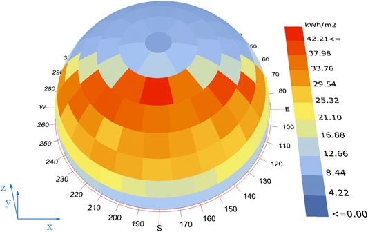
FIGURE 2. Annual total irradiation, visualized for skydome of Geneva, Switzerland. Typical weather data from DOE (2020).

Equation 18 expresses the irradiation coming from one patch $ir{r}^{pt}$ in the coordinates of the skydome $x^{sd},y^{sd},z^{sd}$, where α represents the azimuth angle of the sky-direction and ϵ is the elevation angle of one patch $pt$. Thereby, $x^{sd}$ points to the east, $y^{sd}$ to the north and $z^{sd}$ to the zenith, and the azimuth angle increases clockwise starting from the north, where $\alpha =0$. The elevation angle increases counterclockwise from $\mathit{ϵ}=0$ for patches with no elevation in the sky (compare with Figure 2).

${\overrightarrow{irr}}^{pt}=ir{r}^{pt}\cdot \left(\begin{array}{c}-\sin {\alpha }^{pt}\cdot \cos {\mathit{ϵ}}^{pt}\\ -\cos {\alpha }^{pt}\cdot \cos {\mathit{ϵ}}^{pt}\\ -\sin {\mathit{ϵ}}^{pt}\\ \end{array}\right)\forall \left\{({\alpha }^{pt};{\mathit{ϵ}}^{pt})\right|pt\in \mathbf{P}\}(18)$

Orientation of PV Panel

If $x^{pv},y^{pv},z^{pv}$ define the coordinate system of the PV panel, then $z^{pv}$ is perpendicular to the panel and represents the direction where the irradiation is of relevance for the photoelectric effect, and $x^{pv},y^{pv}$ set up the plane of the PV module itself. Orienting the PV panel in the $x^{sd},y^{sd},z^{sd}$ coordinate system of the skydome means to rotate the PV panel twice. The rotation axis of the azimuth orientation is always the $z^{sd}$ axis of the skydome. In contrast, the tilt rotation is always around the $x^{pv}$ of the panel. If the azimuth rotation is carried out first, the second rotation is around the new ${\tilde{x}}^{pv}$ of the PV panel. If the tilt rotation is carried out first, the $z^{sd}$ axis has to be expressed in dependence of the first rotation around $x^{pv}$. Whereas the azimuth rotation is clockwise (negative), tilt rotation is counterclockwise (positive). This leads to the rotation matrix $\text{Γ}$ shown in Eq. 19.

$\begin{array}{l}{\text{Γ}}_{{\tilde{x}}^{pv}}\cdot {\text{Γ}}_{z^{sd}}={\text{Γ}}_{z^{sd}}{\text{Γ}}_{x^{pv}}=\left[\begin{array}{ccc}\cos {\alpha }^{pv}& -\sin {\alpha }^{pv}& 0\\ \sin {\alpha }^{pv}\cdot \text{cos}{\gamma }^{pv}& \cos {\alpha }^{pv}\cdot \cos {\gamma }^{pv}& -\sin {\gamma }^{pv}\\ \sin {\alpha }^{pv}\cdot \sin {\gamma }^{pv}& \cos {\alpha }^{pv}\cdot \sin {\gamma }^{pv}& \cos {\gamma }^{pv}\end{array}\right]\\ \forall {\alpha }^{pv}\in \mathbf{A},\forall {\gamma }^{pv}\in \mathbf{T}\end{array}(19)$

The combination of Eq. 18 and the rotation matrix $\text{Γ}$ leads to Expression 20 for the incident irradiation density $irr$ along the negative $z^{pv}$ axis of the PV module. Therefore, the pair (${\alpha }^{pt},{\mathit{ϵ}}^{pt}$) uniquely defines the position of one patch $pt$ within the skydome and (${\alpha }^{pv},{\gamma }^{pv}$) the orientation of the PV panel. Taking only positive values allows filtering out the contribution of irradiation coming from behind the panel. The irradiation thus calculated is integrated over the whole skydome.

$\begin{array}{l}ir{r}^{pv}\left({\alpha }^{pv},{\gamma }^{pv}\right)=\left(-1\right)\cdot \underset{pt=1}{{\displaystyle \sum }^P}ir{r}^{pt}\left({\alpha }^{pv},{\gamma }^{pv}\right)\\ =\underset{pt=1}{{\displaystyle \sum }^P}ir{r}^{pt}\cdot \text{max}[(\sin {\alpha }^{pv}\cdot \sin {\gamma }^{pv}\cdot \sin {\alpha }^{pt}\cdot \cos {\mathit{ϵ}}^{pt}+\cos {\alpha }^{pv}\cdot \sin {\gamma }^{pv}\cdot \cos {\alpha }^{pt}\cdot \cos {\mathit{ϵ}}^{pt}+\cos {\gamma }^{pv}\cdot \sin {\mathit{ϵ}}^{pt}),0]\\ \forall {\alpha }^{pv}\in \mathbf{A},\forall {\gamma }^{pv}\in \mathbf{T}\end{array}(20)$

Figure 3 shows the irradiation received by the PV modules, whereas Figure 2 shows a visualization of the irradiation coming from the skydome. For a flat, horizontal panel, the incoming irradiation is independent of the azimuth angle. For azimuth angles, where the Sun is never positioned over the year, annual irradiation density is strictly increasing with lowering the tilt angle and maximal for tilt angle ${\gamma }^{pv}=0$ (horizontal panels). The situation changes for PV orientation between east (azimuth: 90°) and west (azimuth: 270°). Starting from a vertical panel, decreasing the tilt leads to an increase in the irradiation density. The annual irradiation is maximized at a tilt angle of 35°for azimuth 182°, which is around 10% larger than at horizontal irradiation. Between 35° and 0°tilt the irradiation is decreases again until horizontal irradiation.

FIGURE 3

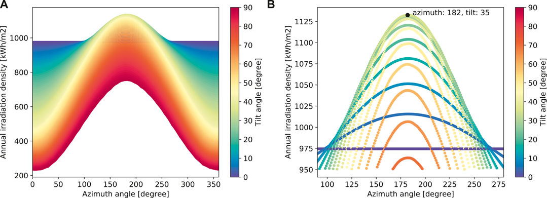
FIGURE 3. (A) Annual irradiation on oriented PV modules in the climate zone of Geneva. (B) Annual irradiation on PV modules oriented between azimuth 80°–280°and greater than 950 kWh/m2, visualization of tilt in 5°steps, azimuth in 1°steps.

Flat Roofs and Shading

On tilted roofs, the panel is considered to occupy only the size of the module itself. Unlike when using tilted roofs, the proposed approach takes into account the actual area $A^{PV}$ occupied by the module on flat roofs. This is calculated as a function of the width of one module $w^{pv}$, the required minimum distance $d^{\beta }$ between PV modules to prevent shading, and the relative tilt angle to the surface ${\gamma }^{pv}$. The distance between two rows of oriented modules is given by Eq. 21. Thereby, $h^{pv}$ is the module height and β is the design limiting angle that avoids shading. The design limiting angle corresponds to the lowest Sun evaluation during solar noon that occurs within a year. Figure 4 illustrates this geometric correlation.

$A^{pv}\left({\gamma }^{pv}\right)=w^{pv}\cdot d=w^{pv}\cdot h^{pv}\cdot \frac{\text{sin}\left({\gamma }^{pv}+\beta \right)}{\text{sin}\left(\beta \right)}\forall {\gamma }^{pv}\in \mathbf{T}(21)$

FIGURE 4

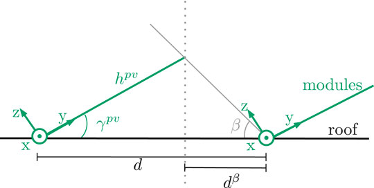
FIGURE 4. Distance d between two modules (green) for a given module height $h^{pv}$, tilt angle ${\gamma }^{pv}$ and sun elevation/liming angle β.

The design limiting angle is not only used for placing the modules on the roof but also for simplification during the determination of incident irradiation. A common assumption is that there is no shading between modules if the placing of the modules respects the design limiting angle (Martinez-Rubio et al., 2015). Simulations confirmed the hypothesis that the irradiation loss from direct irradiation is small, if the limiting angle is respected during placement. However, the diffuse component has a significant share on the losses and leads to a reduction for the tilt with maximum annual yield (e.g., −8°in Geneva) (Mermoud, 2012).

This simplification is not needed when modeling the irradiation with the cumulative sky approach, as described in the previous section. The total irradiation from the partly shaded skydome is reduced by the patches that are not visible from the perspective of the PV module, i.e. that are below the limiting angle. The relative limiting angle is different for each skypatch, since the relative azimuth direction between patch and panel (${\alpha }^{pt}-{\alpha }^{pv}$) varies and therewith the relative distance between the rows $d^{\beta ,\alpha }$. Figure 5 visualizes this geometric relation and Eq. 22 expresses the relative distance between the modules along the relative orientation of the patch.

$\begin{array}{l}{d}^{\beta ,\alpha }=\frac{d^{\beta }}{\text{cos}\left({\alpha }^{pt}-{\alpha }^{pv}\right)}\stackrel{\left(21\right)}{=}\frac{\text{sin}\left({\gamma }^{pv}\right)\cdot h^{pv}}{\text{cos}\left({\alpha }^{pt}-{\alpha }^{pv}\right)\cdot \text{tan}\left(\beta \right)}\\ \forall \beta \ne 0,\forall \{pt\in \mathbf{P}|{\alpha }^{pt}-{\alpha }^{pv}\ne \pm {90}^{\circ }\}\end{array}(22)$

FIGURE 5

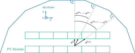
FIGURE 5. Distance d between the modules for determing the inter-modular shading depending on the relative azimuth orientation ${\alpha }^{pt}-{\alpha }^{pv}$.

Distance $d^{\beta ,\alpha }$ yields to the limiting angle ${\beta }^{\alpha }$ along the relative azimuth direction (Eq. 23). The limiting angle ${\beta }^{\alpha }$ is greatest and equal to the design limiting angle β for the patch straight in front of the panel (${\alpha }^{pt}={\alpha }^{pv}$) and then decreases toward the boundaries of the light capture zone.

$\begin{array}{l}\text{tan}\left({\beta }^{\alpha }\right)=\frac{\text{sin}\left({\gamma }^{pv}\right)\cdot h^{pv}}{d^{\beta ,\alpha }}=\text{cos}\left({\alpha }^{pt}-{\alpha }^{pv}\right)\cdot \text{tan}\left(\beta \right)\\ \forall {\alpha }^{pv}\in \mathbf{A},\forall {\gamma }^{pv}\in \mathbf{T},\forall \left\{{\alpha }^{pt}\right|pt\in \mathbf{P}\}\end{array}(23)$

To determine the shaded irradiation, the irradiation from the one patch is piecewise linearized over the evaluation angle of the patch, which varies 12°, with ${\mathit{ϵ}}^{pt}$ marking the central point (Eq. 24). The shading factor of one patch $s^{pt}\in [0;1]$ is equal to zero for completely shaded patches and 1 for completely unshaded patches.

$s^{pt}\left(\beta \right)=\{\begin{array}{ll}0\hfill & {\mathit{ϵ}}^{pt}\le {\beta }^{\alpha }-6\hfill \\ \frac{{\mathit{ϵ}}^{pt}+6-{\beta }^{\alpha }}{12}\hfill & {\beta }^{\alpha }-6<{\mathit{ϵ}}^{pt}<{\beta }^{\alpha }+6\hfill \\ 1\hfill & {\mathit{ϵ}}^{pt}\ge {\beta }^{\alpha }+6\hfill \end{array}\forall \left\{({\alpha }^{pt},{\mathit{ϵ}}^{pt})\right|pt\in \mathbf{P}\}(24)$

Equation 25 gives the partly shaded irradiation in dependence of the chosen design limiting angle β.

$\begin{array}{l}ir{r}^{pv}\left({\alpha }^{pv},{\gamma }^{pv},\beta \right)=\left(-1\right)\cdot \underset{pt=1}{{\displaystyle \sum }^P}{s}^{pt}\left(\beta \right)\cdot ir{r}^{pt}\left({\alpha }^{pv},{\gamma }^{pv}\right)\\ \forall {\alpha }^{pv}\in \mathbf{A},\forall {\gamma }^{pv}\in \mathbf{T}\end{array}(25)$

Figure 6 is presents a visualization of the relative irradiation loss for different design limiting angles. Thereby, the unobscured skydome and the panel in the same orientation give the reference irradiation.

FIGURE 6

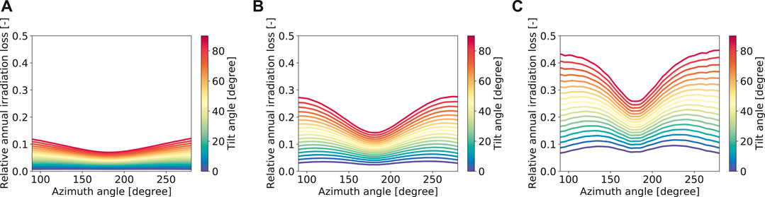
FIGURE 6. Irradiation loss of PV panel shadowing for different design limiting angles β. (A) β = 10 degree, (B) β = 20 degree, (C) β = 30 degree.

The design limiting angle has a significant impact on the received irradiation on the panel. Low angles lead to much lower losses (max around 10% for β = 10°) than do high angles (max around 45% for β = 30°) but also require more surface area of the roof. The losses are less for south oriented panels, since the direct irradiation of the Sun from this direction comes from higher elevation angles.

The proposed approach to model the irradiation losses includes both direct and anisotropic diffuse irradiation, with two simplifications: 1) all rows are considered to be partly shaded, even the front row, and 2) below ${\beta }^{\alpha }$, the whole panel is receives no irradiation, although this is only true for the foot of the panel. The latter simplification implies irradiation losses even for very low tilt angles. As studies show that the electricity generated drastically drops off for partly shaded panels (Mermoud, 2012), this is considered a reasonable assumption.

Input Data and Its Clustering

The large number of annual data points are clustered to typical periods, which represent typical days, and consist of 24 time steps for each hour of the day. Reducing the size of the data representing the energy demand of the building and the climatic conditions of the site is needed in order to make the problem computationally manageable but still represent the operation of a full year. The K- medoids clustering algorithm is therefore used, as this has been commonly used for combined heat and power generation systems (Domínguez-Muñoz et al., 2011). Typical days are identified based on three variables: global irradiation, ambient temperature, and day of the week, of which the latter is important for the electric load profiles of the buildings, since residential buildings show a different trend on weekends than on weekdays. Typical weather data is available from the EnergyPlus open source database (DOE, 2020). Figure 7 shows the quality of the preformed data clustering on global irradiation and ambient temperature for Geneva, Switzerland, with different number of clusters. The share of weekdays per year are represented in every number of clusters.

FIGURE 7

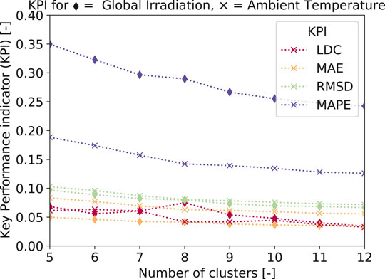
FIGURE 7. KPI for different number of k-medoid clusters: load duration curve (LDC), mean average error (MAE), root mean square deviation (RMSD) and mean average percentage error (MAPE). Selected number of clusters is 10 additional to two extreme periods. Typical weather data for Geneva Switzerland (DOE, 2020).

Based on the information presented in Figure 7, yearly operation was based on 10 typical days, since this appears as a good compromise between the key performance indicators and the expected computational requirements.

Results

MOO Results

The proposed method is applied to a case study in Switzerland. The first study presents a typical residential building with a heated area of 250 m² and a large available roof area consisting of four tilted and one flat surfaces (see Table 1). For determination of the oriented shading losses between PV modules, the design limiting angle β is set to 20°, which represents the lowest Sun evaluation during solar noon for Geneva in Switzerland, occurring on the 21st of December (Hoffmann, 2020). This was chosen as an acceptable trade–off between space requirements and shading losses. Shading losses are below 10% for tilt angles between the horizontal position and those leading to maximum electricity generation (see Figure 6B). The results of the MOO optimization for the reference building are shown in Figures 8, 9.

TABLE 1

TABLE 1. Building parameters for a typical single–family house with large available roof surface.

FIGURE 8

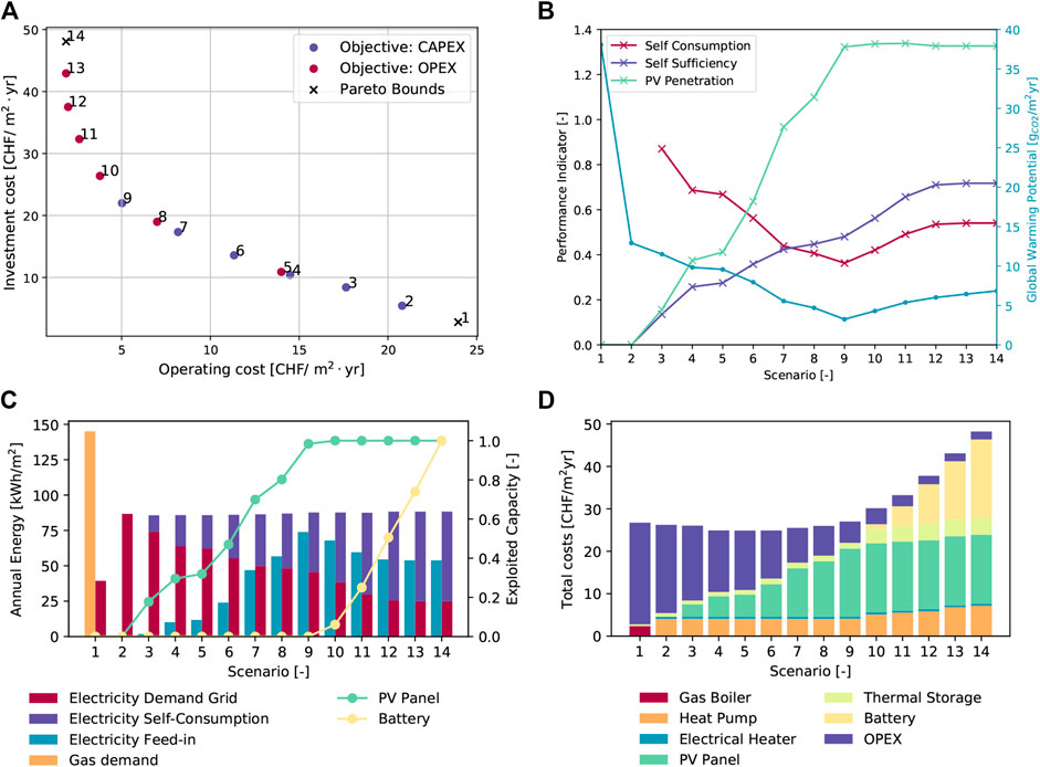
FIGURE 8. Results of MOO of one residential building: (A) definition of Scenarios on pareto curve for investment and operation costs, (B) performance indicator for each scenario, (C) usage of resources, and (D) distribution of total annual cost in identified energy system configurations.

FIGURE 9

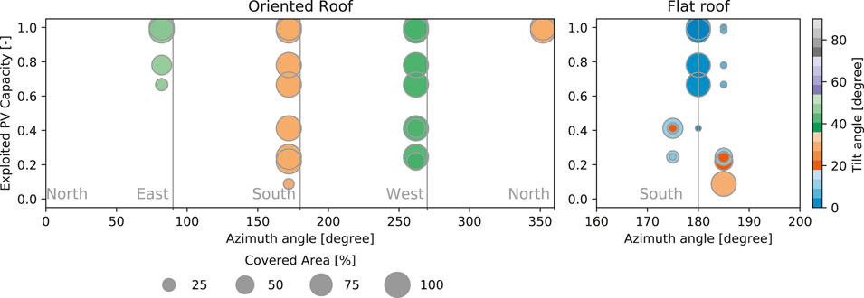
FIGURE 9. Optimal distribution of PV installation for different roofs.

The CAPEX and OPEX for each non-dominated solution on the Pareto front are shown in Figure 8A and are divided by the heated surface of the building to ease comparison. The CAPEX ranged from a minimum of 2.8 CHF/m²yr (Scenario 1) to 48 CHF/m²yr (Scenario 14), whereas the OPEX ranged from 1.9 to 24 CHF/m²yr. The scenario numbers (1–14) are defined as the points on the Pareto curve, ordered from the lowest to the highest CAPEX.

Although all scenarios are optimal from a Pareto perspective when looking at CAPEX and OPEX separately, the analysis of TOTEX tells a different story. As shown in Figure 8D, the resulting TOTEX are similar in Scenarios 1 through 9 at around 27 CHF/m²yr (minimum TOTEX for Scenario 4–6 at 25 CHF/m²yr), whereas they increased rapidly in Scenarios 10–14, reaching a maximum of approximately 50 CHF/m²yr.

The increase in TOTEX in Scenarios 9–14 is due to the fast increase in CAPEX in these scenarios, mostly due to the decision to install batteries (first appearing in Scenario 10), which is not compensated by a commensurate reduction in OPEX. The reason for this trend can be seen in Figure 8C: in Scenarios 3–8, the OPEX are reduced by installing PV panels, hence reducing the electricity demand from the grid, while gradually increasing the electricity feed-in. As the PV capacity saturates, OPEX can be further reduced by increasing the self consumption, because of the price difference between buying electricity from the grid and selling it to the grid. This can be achieved by installing batteries, which allows for a better match between demand and supply. From Scenario 9 to 14, both the electricity demand from the grid and feed-in decrease, meaning that the total amount of energy generated locally remains approximately constant, but it is used for fulfilling the demand rather than sold to the grid.

This can be also observed from the evolution of SS and SC (Figure 8B). The SS gradually increases when the PV panels are installed, and continues increasing even as the PV penetration flattens, because of the use of batteries. On the other hand, the SC first decreases with increasing PV penetration (until Scenario 9), and then begins increasing again as a result of the use of batteries.

Figure 8B also shows the performance of the Pareto-optimal solutions in terms of GWP. The main contribution to reduce the environmental impact of the system comes from the use of heat pumps instead of gas boilers for heating, which reduces the GWP from approximately 37 to 13 g Co₂ eq/m²yr. The addition of PV panels provides a significant contribution to reducing CO₂ emissions, which reaches a minimum of 3.2 g Co₂ eq/m²yr in Scenario 9. From then onward, the use of batteries has the opposite effect, because of the losses in the charge/discharge cycle and of the large GHG emissions connected to the battery production process.

Concerning other technologies installed, thermal energy storage is used in most scenarios. A relatively small thermal storage is installed in Scenarios 2–9; whereas in Scenarios 10–14 larger systems are installed, following the same principle as for the batteries.

Additional information related to the installation of PV panels is provided in Figure 9. These results start providing insights related to the main topic of this paper. For low installed PV capacity, panels are equipped on the flat and on the south-oriented roof. On the flat roof, the panels are positioned with a south orientation and with a 30°tilt, according to common practice. However, at even a small increase in the total installed PV capacity, the west-oriented roof is used over the east-oriented roof, and the azimuth and tilt of the panels installed on the flat roof changes. This is likely because west-oriented panels provide a better match between supply and demand than do east-oriented panels. Finally, in Scenario 14, the east facing and the north facing roofs are also covered with PV panels, whereas the panels placed on the flat roof are installed with 0°tilt angle to minimize shading effects between panels, hence allowing for the installation of more PV modules on the same roof area.

Optimal Orientation and the Role of Self-Consumption

One additional objective of this study is to determine the effect of the interaction between the hourly variation of the thermal and electrical demand, the energy system, and the choice of the surface where the solar panels are installed.

The results shown in Figure 9 serve as an excellent starting point for this discussion. Although the south-facing rooftops are selected first, west-facing surfaces are chosen over east-facing surfaces. . This was further explored in the case of a building with no tilted roofs: in this case, the optimizer has full freedom of choice in terms of orientation and tilt, rather than being forced to choose among a limited set of options, and can therefore provide more insight.

These results are presented in Figure 10. Figure 10A refers to the reference pricing case of 0.24 CHF/kWh for electricity purchased from the grid and a feed-in tariffs of 0.08 CHF/kWh, whereas Figure 10B refers to the same case but with a 0 CHF/kWh feed-in price. As expected, given its highest yearly energy generation, south-oriented panels are preferred; however, at feed-in tariffs of 0 CHF/kWh, the panels are slightly oriented toward the west and have a higher tilt, especially in the cases with a lower total installed PV capacity.

FIGURE 10

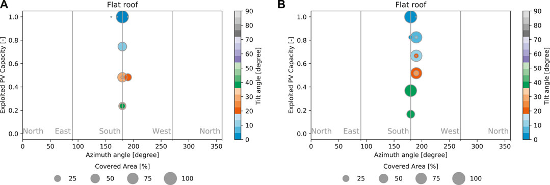
FIGURE 10. Optimal PV orientation for different installed capacities on a flat roof: (A) cost optimal placement for an electricity price of 0.24 CHF/kWh and feed-in tariffs of 0.08 CHF/kWh, and (B) optimal placement for self consumption for an electricity price of 0.24 CHF/kWh and feed-in tariffs of 0 CHF/kWh.

In most residential buildings, the main energy demand is in the evening, when people are at home, and during the heating season in winter, when the Sun is lower in the sky, thus explaining this orientation shift. However, this effect is minor, since the developed model includes optimal scheduling. This leads to the conclusion that, although this effect does not seem to have a substantial influence on the overall performance, the common practice of installing PV panels with the azimuth and tilt that maximizes energy generation may not be the best choice, especially when the objective is to maximize self-consumption. This trend is only seen for scenarios where only parts of the roofs are covered with PV panels: when the whole roof is covered, the optimizer prioritizes the maximization of the yearly generation, thus favoring azimuth and tilt angles that minimize shading among panels.

Comparison With Flat Roof Assumption

This work also aimed to provide an estimation of the error generated by assuming horizontal panels on the entire roof surface when attempting to estimate the PV potential from distributed generation. Although this assumption allows a simpler analysis and can rely on more limited set of information, it also introduces error.

The extent of the deviation between the “simplified” and “detailed” approaches for the 40 buildings with individual roofs and load profiles is shown in Figure 11A. For low exploited PV capacity, the general trend is that the best surfaces are used, and, whenever possible, the tilt angle is selected to maximize the yearly energy generation. As a result, the simplified assumption of panels installed with zero azimuth and tilt causes an underestimation of the generated electricity, and a consequent overestimation of the overall operational expenses. As “worse” roofs are used, the error is reduced, until the error sign reverses; for very high levels of PV penetration, as west-, east- and north-oriented roofs are exploited, the simplified flat panel assumption instead becomes an overestimation of the total capacity. While the error largely depends on the individual case, it generally ranges between −12 and +20% for the generated electricity, and −20% and +20% for the operational expenses.

FIGURE 11

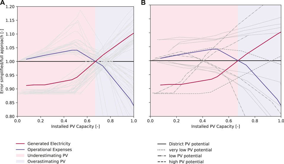
FIGURE 11. Error caused by assuming horizontal PV panels to optimal PV orientation for a district (colored lines) of 40 buildings (gray lines); Buildings with (A) average behavior (B) outlier behavior.

Unlike the estimation of generated electricity, the error seen in the estimated operating expenses does not increase monotonically, but peaks at approximately 50% PV capacity. This can be explained by the difference in feed–in and electricity prices. The error in the estimation of the operational expenses is low in systems with low PV capacity. Here, SC is highest and can be maximized with the optimal scheduling of electrical loads. At some point, these scheduling measures are fully exploited in case of the simplified approach, all additional generated electricity is completely fed into the grid. In contrast, in the full approach “worse” roofs are used, which generate less electricity but lead to a better match of demand and supply profiles. Hence, it leads to further increase of self consumption, causing the peak of overestimating costs at 50% PV capacity. After this point, the limit of self consumption in the full approach is reached and the overproduction of electricity in the simplified approach is so high, that the revenues from the feed-in tariffs decrease the electricity bill drastically.

Whereas Figure 11A shows the behavior of “average” buildings, Figure 11B shows some outliers, i.e. buildings that behave remarkably differently from the rest. In the case of buildings with very high PV potential, the simplified approach tends to always underestimate the potential. Buildings with completely flat roofs are an example of this case: here, in almost all scenarios, the optimal placement involves using panels with a 30° tilt, which generates more energy than the flat case. On the other hand, when the PV potential of the building is very low, the electricity generated in the simplified approach is always overestimated; this can be the case of a house with a pitched roof facing east and west, where all available surfaces have a lower potential compared to a flat roof and, hence, the simplified approach tends to always overestimate the potential.

Impact on the Grid

The main rationale for not following the common practice of installing PV panels with azimuth and tilt that maximize yearly energy generation is related to the benefits that this gives toward maximizing SC. For a system connected to the grid, the maximizing SC helps to balance the grid and thus avoids excessive swings in the use of centralized power generation units. This aspect can become crucial once renewable energy sources (especially uncontrollable ones, such as wind and solar power) take up a significant share of the national energy mix.

Figure 12 allows getting a better understanding of this point, and of how it is connected to the matter of PV panels installation on top of roofs. Here, as demonstrated from the deviation between the energy generated by the optimal system (solid purple line) installed on a real roof and the energy generated by a hypothetical system with all panels oriented south with a 30°angle (dashed purple line), the error, that is generated by not considering the orientation of the PV panels, is apparent. With a ratio of surface area of installed PV panels to the heated surface of just under 50%, the yearly demand of the building can be satisfied locally.

FIGURE 12

FIGURE 12. (A) The need of PV panels of a typical residential building in Switzerland to reach self-sufficiency with re-import. (B) Revenues as a function of installed PV capacity and grid efficiency from the perspective of the grid. The grid buys electricity at a feed-in tariffs of 0.08 CHF/kWh and resells for electricity price 0.24 CHF/kWh.

However, this perspective considers the grid as a perfect energy storage system. As shown by the actual value of the PV electricity that is self-consumed, most of the generated electricity is sold to the grid, and then purchased back when needed. The share of the demand that is satisfied with the energy generated from the PV panels increases with the PV surface installed; however, this share saturates at around 50% of the demand.

From the point of view of each individual prosumer, the grid can be seen as a battery that is able to absorb excess energy from distributed generation and sell it back when the demand exceeds the generation. There are several ways for the grid to fulfill this role: pumped hydroelectric storage is the most commonly used (Akinyele and Rayudu, 2014; Gür, 2018), whereas the use of large battery systems is still limited to few cases, and other technologies (such as compressed air storage or hydrogen) are yet to reach market maturity. Based on this an estimation of the PV system size required for a reference residence to achieve a net zero balance between energy locally generated and consumed for different values of the average efficiency of the storage is shown in Figure 12A. This assumption has a dramatic influence on the surface required for energy balance: for ${\eta }_{\text{grid}-\text{as}-\text{storage}}=0.85$ (which would be the case of lithium-ion batteries), the overall surface required would only slightly increase from the ${\eta }_{\text{grid}-\text{as}-\text{storage}}=1$ assumption. If, however, a much lower efficiency is assumed (${\eta }_{\text{grid}-\text{as}-\text{storage}}=0.40$, which would be in the range of what can be expected when using hydrogen for energy storage), the surface of PV panels installed to reach self-sufficiency is almost doubled.

The effects of the efficiency of the grid as storage for the grid operators can be observed in Figure 12B, based on the assumption of 24/8 ct/kWh for electricity purchased from/sold to the grid. When ${\eta }_{\text{grid}-\text{as}-\text{storage}}$ is high, most of the energy purchased from the prosumers is able to be sold back, and hence the profit is large. With a lower ${\eta }_{\text{grid}-\text{as}-\text{storage}}$, the profits decreases dramatically from the perspective of the grid.

The common interest in efficient grid infrastructure is revealed by Figure 12. From the perspective of the grid operator, profits can be higher as less energy is lost in the charge–discharge cycle, and these profits can be used to reinvest into upgrading the grid itself, generating a positive, cyclic effect. From the perspective of the building energy system, self-sufficiency can be achieved with a lower surface of PV panels installed (and, hence, with lower investment costs) and the supply is more secure, since there is 75% less traffic in the network.

The investigation of a different way to deal with the limitations of the grid is shown in Figure 13. One solution would be to increase the level of self-consumption. The effect of taking into account the effect of the grid-balance constraint on the installation decision of PV panels and on the preferred azimuth and tilt is shown in Figures 13A,B. Here, two alternative means from the perspective of the grid operator implemented to reduce the perturbations generated on the grid by individual prosumers: limiting the amplitude of power variations compared with an average value, or reducing ratio between the feed-in tariffs and electricity cost. Only one solution of the Pareto front is included here, i.e., that which minimizes the TOTEX.

FIGURE 13

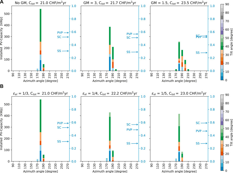
FIGURE 13. Distribution of PV installation and orientation for total cost optimization of 40 buildings with individual load profiles. Assumption of flat roof with unconstrained orientation possibilities. (A) Three different grid constraints. (B) Three different electricity price shares ${\mathit{ϵ}}_{el}$ = feed-in tariff/electricity price.

The results of the first strategy are shown in Figure 13A. When no limitation is applied (left plot), almost all PV panels are installed facing south: with no limitation to the power exchanged with the grid, the optimizer selects the configuration that maximizes energy generation. When a limited restriction is applied (GM = 3, center plot), there is a clear shift toward the west; even though the variation only referred to less then half of the installed PV capacity and for only 10°rotation,a clear trend is visible. This is confirmed when a stricter limitation on grid exchanges is imposed (GM = 1.5, right plot), where less than half of the panels are installed toward south and the average rotation toward the west is even higher. However, this has a relatively small effect on the SC, which only increases from 0.52 to 0.54.

The results of changing the relative price between energy purchased from and sold to the grid is shown in Figure 13B. The effect on the azimuth is less evident, but still present. However, a more distinct effect on the tilt angle is seen, which tends to increase (from 30° to 40°). Also, it appears that the effect on the SC is higher in this case (it increases from 0.52 to 0.59), which may be related to the fact that for electrified heating systems, the electricity demand is highest during winter, where the Sun is lower in the sky. Hence, by increasing the tilt angle, SC can be increased.

The analysis of a district with 40 buildings with individual roof orientation and demand profiles demonstrates that the best economic performance is achieved with around 40% rooftop occupancy, as shown in Figure 14. Even though the optimal orientation is impacted by the orientation of available surfaces, the previous trend of different policies can be confirmed in Figure 14A as well as in Figure 14B.

FIGURE 14

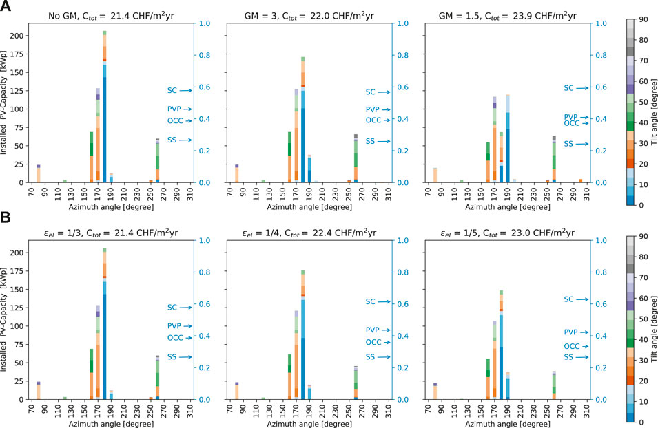
FIGURE 14. Distribution of PV installation and orientation for total cost optimization of 40 buildings with individual load profiles and real roof orientations. occupancy (OCC) (A) Three different Grid constraints. (B) Three different electricity price shares ${\mathit{ϵ}}_{el}$ = feed-in tariff/electricity price.

Conclusion

This work analyzes the influence of the orientation of PV panels on the design and performance of BESs. Existing literature in the field of BES optimization has mainly considered horizontal PV modules and has based the decision of purchasing them on global irradiation without shadowing effects.This work therefore aims to estimate the influence of using different orientations, both from the perspective of the individual building and of the grid, and provide a methodology for selecting which roofs should be covered first. The results confirm the validity of the common assumption of the favorability of south-oriented modules with an approximate tilt of 30°. However, this does not hold true when resources are available for more modules or when the focus shifts to clusters of buildings. To optimize (SC), the optimal orientation is further west and with higher tilt than the standard solution. To maximize the PV capacity on the roof, the use of horizontal panels maximizes the usable roof area.

The most interesting results, however, are related to the interaction with the grid. For higher levels of PV penetration, the role of the grid becomes crucial. Grid operators have the power to influence the quantity as well as the quality of grid exchange by acting in different directions:

Grid efficiency: High grid efficiency is a common interest for both the building owner and the grid operator. With an 85% grid efficiency, a residential building would need around half of its heated surface in area of PV modules to be self sufficient. The point of SS also marks the maximum grid revenue at almost 7 CHF/m²yr. A lower round–trip efficiency requires more PV panels to achieve SS, generates a greater stress on the grid, and reduces annual grid revenues.

Feed-in: The pricing of the electricity exchange with the grid is influences the feed-in to the grid. For lower feed–in prices (or higher demand prices), the most economic solution is to increase tilt angles and slightly lower the PV penetration. This increases SC for a constant level of SS (Figure 13B).

Peak power: Constraining the peak power of the grid exchange leads to a variation in azimuth angles. By moving panels 20°westward and optimally scheduling the operation, the peak can be reduced by 50% while total costs increase by 8.3%.

Even though the optimal orientation strategy is impacted by the orientation of available surfaces, the trend of different grid policies is confirmed by analyzing a 40-building district with individual roof orientation and demand profiles. Comparing the resulting optimally oriented and horizontally oriented panels indicates that the latter generated high error in the estimation of the PV performance. Assuming horizontal panels, causes an overestimation in operating costs by approximately 5 and a 10% underestimation in generated electricity for low PV surfaces. For greater PV surfaces installed, the trend is reversed, and the relative error can increase to up to 20%.

Data Availability Statement

The raw data supporting the conclusions of this article will be made available by the authors, without undue reservation.

Author Contributions

LM Main author, conception and design of the work. Data collection, analysis and interpretation. Developer of applied methods and generating/plotting results. Drafting the article. FB Author, developer of methods, Drafting the article, Critical revision of the article. PS Expert on the part of building energy systems, developer of the building model, critical revision of the article. FM Supervising Professor, conception and design of the work, critical revision of the article.

Funding

This project is carried out within the frame of the Swiss Centre for Competence in Energy Research on the Future Swiss Electrical Infrastructure (SCCER-FURIES) with the financial support of the Swiss Innovation Agency (Innosuisse—SCCER program).

Conflict of Interest

The authors declare that the research was conducted in the absence of any commercial or financial relationships that could be construed as a potential conflict of interest.

Supplementary Material

The Supplementary Material for this article can be found online at: https://www.frontiersin.org/articles/10.3389/fenrg.2020.573290/full#supplementary-material.

Abbreviations

BES building energy system; CAPEX capital expenses; DHW domestic hot water; GIS geographic information systems; GM grid multiple; GWP global warming potential; IPCC Intergovernmental Panel on Climate Change; KPI key performance indicator; LDC load duration curve; MAE mean average error; MAPE mean average percentage error; MILP mixed-integer linear programming; MOO multi-objective optimization; OCC occupancy; OPEX operational expenses; PV photovoltaic; PVP photovoltaic penetration; RMSD root mean square deviation; SC self-consumption; SH space heating; SS self-sufficiency; TOTEX total expenses.

NOMENCLATURE

Parameter

α Azimuth angle °

β Design limiting angle °

δ Temperature coefficient K⁻¹

ε Elevation angle °

${\mathit{\epsilon }}_{\mathit{G}\mathit{M}}$ Upper bound grid multiple -

η Efficiency -

γ Tilt angle °

ν Absorption coefficient -

A Area m²

b Baremodule ‐

c Energy tariff CHF/kWh

d Distance m

${\mathit{d}}_{\mathit{p}}$ Frequency of periods per year d/yr

${\mathit{d}}_{\mathit{t}}$ Frequency of timesteps per period h/d

g Global warming potential streams kg_CO2,eq/kWh

h Height m

i Interest rate ‐

${\mathit{i}}^{\mathit{c}1}$ Fixed Investment Cost CHF

${\mathit{i}}^{\mathit{c}2}$ Continuous Investment Cost CHF/ $\diamond$

${\mathit{i}}^{\mathit{g}1}$ Fixed impact factor kg_CO2,eq

$i^{\mathit{g}2}$ Continuous impact factor kg_CO2,_eq/ $\diamond$

$irr$ Irradiation density kWh/m²

l Lifetime yr

n Project horizon yr

$\mathit{o}\mathit{c}\mathit{c}$ Occupancy share ‐

${\mathit{p}}_{\mathit{d}}$ Period duration h

s Shading factor -

T Temperature K

U Heat transfer coefficient kW/m²K

w Width m

$\mathit{x},\mathit{y},\mathit{z}$ Coordinates ‐

Variables

$\mathit{C}$ Cost CHF

$\mathit{E}$ Electricity kW(h)

$\mathit{f}$ Sizing variable $\diamond$

$\mathit{G}$ Global warming potential kg_CO2,_eq

$\mathit{H}$ Natural gas kW

$\mathit{n}$ Number, quantity -

$\mathit{y}$ Decision variable, binary [−]

Sets

A Azimuth α

C Configuration c

P Patch pt

P Period p

R Replacement r

S Surface s

T Tilt γ

T Timestep t

U Utility u

Superscripts

$+$ Supply

$-$ Demand

$bes$ Building energy system

$cap$ Capital

$el$ Electricity

$ext$ External

$gr$ Grid

$inv$ Investment

$lca$ Life cycle assessment

$ng$ Natural Gas

$op$ Operation

$pv$ Photovoltaic Panel

$ref$ Reference

$rep$ Replacement

$sd$ Skydome

Other

$\text{Γ}$ Rotation Matrix.

References

Akinyele, D. O., and Rayudu, R. K. (2014). Review of energy storage technologies for sustainable power networks. Sustain. Energy Technol. Assess 8, 74–91. doi:10.1016/j.seta.2014.07.004

CrossRef Full Text | Google Scholar

Ashouri, A. (2014). Simultaneous design and control of energy systems. PhD thesis, Zürich (Switzerland) ETH Zurich. doi:10.3929/ethz-a-010210627

CrossRef Full Text | Google Scholar

Assouline, D., Mohajeri, N., and Scartezzini, J.-L. (2017). Quantifying rooftop photovoltaic solar energy potential: a machine learning approach. Sol. Energy 141, 278–296. doi:10.1016/j.solener.2016.11.045

CrossRef Full Text | Google Scholar

Badescu, V. (2008). Modeling Solar Radiation at the Earth’s Surface: Recent Advances (Berlin, Germany: Springer).

Bremer, M., Mayr, A., Wichmann, V., Schmidtner, K., and Rutzinger, M. (2016). A new multi-scale 3D-GIS-approach for the assessment and dissemination of solar income of digital city models. Comput. Environ. Urban Syst. 57, 144–154. doi:10.1016/j.compenvurbsys.2016.02.007

CrossRef Full Text | Google Scholar

Chwieduk, D. A. (2009). Recommendation on modelling of solar energy incident on a building envelope. Renew. Energy 34, 736–741. doi:10.1016/j.renene.2008.04.005

CrossRef Full Text | Google Scholar

Doe, (2020). Weather Data | EnergyPlus, U.S. Department of Energy’s (DOE) Building Technologies Office (BTO) and National Renewable Energy Laboratory (NREL). Available at:https://energyplus.net/weather.

Google Scholar

Domínguez-Muñoz, F., Cejudo-López, J. M., Carrillo-Andrés, A., and Gallardo-Salazar, M. (2011). Selection of typical demand days for CHP optimization. Energy Build. 43, 3036–3043. doi:10.1016/j.enbuild.2011.07.024

CrossRef Full Text | Google Scholar

J. A. Duffie, and W. A. Beckman (Editors) (2013). Solar engineering of thermal processes. 4th Edn. Hoboken, NJ: John Wiley.

CrossRef Full Text

Fan, Y., and Xia, X. (2017). A multi-objective optimization model for energy-efficiency building envelope retrofitting plan with rooftop PV system installation and maintenance. Appl. Energy 189, 327–335. doi:10.1016/j.apenergy.2016.12.077

CrossRef Full Text | Google Scholar

Fazlollahi, S., Bungener, S. L., Mandel, P., Becker, G., and Maréchal, F. (2014). Multi-objectives, multi-period optimization of district energy systems: I. Selection of typical operating periods. Comput. Chem. Eng. 65, 54–66. doi:10.1016/j.compchemeng.2014.03.005

CrossRef Full Text | Google Scholar

Freitas, S., Catita, C., Redweik, P., and Brito, M. C. (2015). Modelling solar potential in the urban environment: state-of-the-art review. Renew. Sustain. Energy Rev. 41, 915–931. doi:10.1016/j.rser.2014.08.060

CrossRef Full Text | Google Scholar

Gür, T. M. (2018). Review of electrical energy storage technologies, materials and systems: challenges and prospects for large-scale grid storage. Energy Environ. Sci. 11, 2696–2767. doi:10.1039/C8EE01419A

CrossRef Full Text | Google Scholar

Girardin, L. (2012). A GIS-based methodology for the evaluation of integrated energy systems in urban area. PhD. thesis. Lausanne (Switzerland): EPFL. doi:10.5075/epfl-thesis-5287

CrossRef Full Text | Google Scholar

Global Alliance for Buildings and Construction, International Energy Agency and the United Nations Environment Programme (2019). 2019 global status report for buildings and construction: towards a zero-emission, efficient and resilient buildings and construction sector.

CrossRef Full Text | Google Scholar

Hafez, A. Z., Soliman, A., El-Metwally, K. A., and Ismail, I. M. (2017). Tilt and azimuth angles in solar energy applications–a review. Renew. Sustain. Energy Rev. 77, 147–168. doi:10.1016/j.rser.2017.03.131

CrossRef Full Text | Google Scholar

Hartner, M., Kollmann, A., Haas, R., and Mayr, D. (2017). Optimal sizing of residential PV-systems from a household and social cost perspective. Sol. Energy 141, 49–58. doi:10.1016/j.solener.2016.11.022

CrossRef Full Text | Google Scholar

Hoffmann, T. (2020). SunCalc sun position- und sun phases calculator. Library Catalog. Available at: www.suncalc.org.

Google Scholar

Holweger, J., Bloch, L., Ballif, C., and Wyrsch, N. (2019a). Mitigating the impact of distributed PV in a low-voltage grid using electricity tariffs. arXiv:1910.09807 [cs, eess] ArXiv: 1910.09807. Available at: https://arxiv.org/abs/1910.09807.

Google Scholar

Holweger, J., Dorokhova, M., Bloch, L., Ballif, C., and Wyrsch, N. (2019b). Unsupervised algorithm for disaggregating low-sampling-rate electricity consumption of households. Sustain. Energy, Grids Netw. 19, 100244. doi:10.1016/j.segan.2019.100244

CrossRef Full Text | Google Scholar

Jennings, M., Fisk, D., and Shah, N. (2014). Modelling and optimization of retrofitting residential energy systems at the urban scale. Energy 64, 220–233. doi:10.1016/j.energy.2013.10.076

CrossRef Full Text | Google Scholar

Jing, R., Wang, M., Liang, H., Wang, X., Li, N., Shah, N., et al. (2018). Multi-objective optimization of a neighborhood-level urban energy network: considering Game-theory inspired multi-benefit allocation constraints. Appl. Energy 231, 534–548. doi:10.1016/j.apenergy.2018.09.151

CrossRef Full Text | Google Scholar

Kantor, I., Robineau, J.-L., Bütün, H., and Maréchal, F. (2020). A mixed-integer linear programming formulation for optimizing multi-scale material and energy integration. Front. Energy Res. 8, 49. doi:10.3389/fenrg.2020.00049

CrossRef Full Text | Google Scholar

Khoo, Y. S., Nobre, A., Malhotra, R., Yang, D., Ruther, R., Reindl, T., et al. (2014). Optimal orientation and tilt angle for maximizing in-plane solar irradiation for PV applications in Singapore. IEEE J. Photovoltaics 4, 647–653. doi:10.1109/JPHOTOV.2013.2292743

CrossRef Full Text | Google Scholar

Klauser, D. (2016). Solarpotentialanalyse für Sonnendach.ch Schlussbericht. Bern, Schweiz: Eidgenössisches Departement für Umwelt, Verkehr, Energie und Kommunikation UVEK, Bundesamt für Energie. Available at: https://pubdb.bfe.admin.ch/de/publication/download/8196

Google Scholar

Ko, L., Wang, J.-C., Chen, C.-Y., and Tsai, H.-Y. (2015). Evaluation of the development potential of rooftop solar photovoltaic in Taiwan. Renew. Energy 76, 582–595. doi:10.1016/j.renene.2014.11.077

CrossRef Full Text | Google Scholar

Lahnaoui, A., Stenzel, P., and Linssen, J. (2017). Tilt angle and orientation impact on the techno-economic performance of photovoltaic battery systems. Energy Procedia 105, 4312–4320. doi:10.1016/j.egypro.2017.03.903

CrossRef Full Text | Google Scholar

Laveyne, J. I., Bozalakov, D., Van Eetvelde, G., and Vandevelde, L. (2020). Impact of solar panel orientation on the integration of solar energy in low-voltage distribution grids. Int. J. Photoenergy, 2020, 1–13. doi:10.1155/2020/2412780

CrossRef Full Text | Google Scholar

Lazar, J. (2016). Teaching the “Duck” to Fly. 2nd Edn. Montpelier VT: Regulatory Assistance Project.

Litjens, G. B. M. A., Worrell, E., and van Sark, W. G. J. H. M. (2017). Influence of demand patterns on the optimal orientation of photovoltaic systems. Sol. Energy 155, 1002–1014. doi:10.1016/j.solener.2017.07.006

CrossRef Full Text | Google Scholar

Lucon, O. (2014). “Buildings,” in Climate change 2014: mitigation of climate change. Contribution of working group III to the fifth assessment report of the intergovernmental panel on climate change New York, NY: Cambridge University Press.

Google Scholar

Luthander, R., Widén, J., Nilsson, D., and Palm, J. (2015). Photovoltaic self-consumption in buildings: a review. Appl. Energy 142, 80–94. doi:10.1016/j.apenergy.2014.12.028

CrossRef Full Text | Google Scholar

Ma, T., Wu, J., Hao, L., Lee, W.-J., Yan, H., and Li, D. (2018). The optimal structure planning and energy management strategies of smart multi energy systems. Energy 160, 122–141. doi:10.1016/j.energy.2018.06.198

CrossRef Full Text | Google Scholar

Martinez-Rubio, A., Sanz-Adan, F., and Santamaria, J. (2015). Optimal design of photovoltaic energy collectors with mutual shading for pre-existing building roofs. Renew. Energy 78, 666–678. doi:10.1016/j.renene.2015.01.043

CrossRef Full Text | Google Scholar

Mermoud, A. (2012). "Optimization of row-arrangement in PV systems, shading loss evaluations according to module positioning and connexions,"in Proceedings of the 27th european photovoltaic solar energy conference and exhibition, Frankfurt, Germany, September 2012. doi:10.4229/27THEUPVSEC2012-5AV.1.46

CrossRef Full Text | Google Scholar

Mondol, J. D., Yohanis, Y. G., and Norton, B. (2007). The impact of array inclination and orientation on the performance of a grid-connected photovoltaic system. Renew. Energy 32, 118–140. doi:10.1016/j.renene.2006.05.006

CrossRef Full Text | Google Scholar

Morvaj, B., Evins, R., and Carmeliet, J. (2016). Optimising urban energy systems: simultaneous system sizing, operation and district heating network layout. Energy 116, 619–636. doi:10.1016/j.energy.2016.09.139

CrossRef Full Text | Google Scholar

Pachauri, R. K., Allen, M. R., Barros, V. R., Broome, J., Cramer, W., Christ, R., et al. (2014). Climate Change 2014: Synthesis Report. Contribution of Working Groups I, II and III to the Fifth Assessment Report of the Intergovernmental Panel on Climate Change. Geneva, Switzerland: IPCC.

Perez, R., Seals, R., and Michalsky, J. (1993). All-weather model for sky luminance distribution-Preliminary configuration and validation. Sol. Energy 50, 235–245. doi:10.1016/0038-092X(93)90017-I

CrossRef Full Text | Google Scholar

Portmann, M., Galvagno-Erny, D., Lorenz, P., Schacher, D., and Heinrich, R. (2019). Sonnendach.ch und Sonnenfassade.ch: berechnung von Potenzialen in Gemeinden. Bundesamt für Energie BFE, Bern Techinal report.

Google Scholar

Rager, J. M. F. (2015). Urban energy system design from the heat perspective using mathematical programming including thermal storage. PhD. thesis. Lausanne (Switzerland): EPFL. doi:10.5075/epfl-thesis-6731

CrossRef Full Text | Google Scholar

Rhodes, J. D., Upshaw, C. R., Cole, W. J., Holcomb, C. L., and Webber, M. E. (2014). A multi-objective assessment of the effect of solar PV array orientation and tilt on energy production and system economics. Sol. Energy 108, 28–40. doi:10.1016/j.solener.2014.06.032

CrossRef Full Text | Google Scholar

Robinson, D., and Stone, A. (2004). “Irradiation modelling made simple: the cumulative sky approach and its applications,” in Proceedings of the 21st PLEA conference, Eindhoven, The Netherlands, September 2004

Google Scholar

Sadineni, S. B., Atallah, F., and Boehm, R. F. (2012). Impact of roof integrated PV orientation on the residential electricity peak demand. Appl. Energy 92, 204–210. doi:10.1016/j.apenergy.2011.10.026

CrossRef Full Text | Google Scholar

Sadineni, S. B., Atallah, F., and Boehm, R. F. (2012). Impact of roof integrated PV orientation on the residential electricity peak demand. Appl. Energy 92, 204–210. doi:10.1016/j.apenergy.2011.10.026

CrossRef Full Text | Google Scholar

Schüler, N. C. (2018). Computational methods for multi-criteria decision support in urban planning. PhD. thesis. Lausanne (Switzerland): EPFL. doi:10.5075/epfl-thesis-8877

CrossRef Full Text | Google Scholar

Shukla, K. N., Rangnekar, S., and Sudhakar, K. (2015). Comparative study of isotropic and anisotropic sky models to estimate solar radiation incident on tilted surface: a case study for Bhopal, India. Energy Rep. 1, 96–103. doi:10.1016/j.egyr.2015.03.003

CrossRef Full Text | Google Scholar

Sia, (2015). 2024:2025 Raumnutzungsdaten für die Energie- und Gebäudetechnik. Zürich, Switzerland: Schweizerischer Ingenieur und Aarchitektenverein.

Stadler, M., Groissböck, M., Cardoso, G., and Marnay, C. (2014). Optimizing distributed energy resources and building retrofits with the strategic DER-CAModel. Appl. Energy 132, 557–567. doi:10.1016/j.apenergy.2014.07.041

CrossRef Full Text | Google Scholar

Stadler, P., Girardin, L., Ashouri, A., and Maréchal, F. (2018). Contribution of model predictive control in the integration of renewable energy sources within the built environment. Front. Energy Res. 6, 22. doi:10.3389/fenrg.2018.00022

CrossRef Full Text | Google Scholar

Stadler, P. M. (2019). Model-based sizing of building energy systems with renewable sources. PhD. thesis. Lausanne (Switzerland): EPFL. doi:10.5075/epfl-thesis-9560

CrossRef Full Text | Google Scholar

Turton, R. (2012). Analysis, synthesis, and design of chemical processes. 4th Edn. Upper Saddle River, NJ: Prentice-Hall.

van der Stelt, S., AlSkaif, T., and van Sark, W. (2018). Techno-economic analysis of household and community energy storage for residential prosumers with smart appliances. Appl. Energy 209, 266–276. doi:10.1016/j.apenergy.2017.10.096

CrossRef Full Text | Google Scholar

Verso, A., Martin, A., Amador, J., and Dominguez, J. (2015). GIS-based method to evaluate the photovoltaic potential in the urban environments: the particular case of Miraflores de la Sierra. Sol. Energy 117, 236–245. doi:10.1016/j.solener.2015.04.018

CrossRef Full Text | Google Scholar

Vulkan, A., Kloog, I., Dorman, M., and Erell, E. (2018). Modeling the potential for PV installation in residential buildings in dense urban areas. Energy Build. 169, 97–109. doi:10.1016/j.enbuild.2018.03.052

CrossRef Full Text | Google Scholar

Walch, A., Mohajeri, N., and Scartezzini, J.-L. (2019). A critical comparison of methods to estimate solar rooftop photovoltaic potential in Switzerland. J. Phys.: Conf. Ser. 1343, 012035. doi:10.1088/1742-6596/1343/1/012035

CrossRef Full Text | Google Scholar

Wernet, G., Bauer, C., Steubing, B., Reinhard, J., Moreno-Ruiz, E., and Weidema, B. (2016). The ecoinvent database version 3 (part I): overview and methodology. Int. J. Life Cycle Assess. 21, 1218–1230. doi:10.1007/s11367-016-1087-8

CrossRef Full Text | Google Scholar

Wu, R., Mavromatidis, G., Orehounig, K., and Carmeliet, J. (2017). Multiobjective optimisation of energy systems and building envelope retrofit in a residential community. Appl. Energy 190, 634–649. doi:10.1016/j.apenergy.2016.12.161

CrossRef Full Text | Google Scholar