Deriving Economic Potential and GHG Emissions of Steel Mill Gas for Chemical Industry

Introduction

Greenhouse gas (GHG) emissions such as CO₂ from industry continue to rise worldwide despite efforts to decrease emissions, such as stated in the 2015 Paris agreement, which aims to limit global warming to 2°C and make efforts to limit it to 1.5°C (Jarraud and Steiner, 2014; IEA, 2017; Rogelj et al., 2018). The steel industry is one of the major emitters of CO₂, with the sector being responsible for around 6% of total CO₂ emissions globally, making it also the largest industrial emitter. Additionally, the industry grew by 6.9% annually between 2000 and 2014 (He and Wang, 2017; World Steel Association, 2020) and is expected to reach 2200 Mt of crude steel production in 2050 (Bellevrat and Menanteau, 2009), primarily due to demand in developing countries for infrastructure. Therefore, the industry’s emissions are predicted to increase naturally in the mid-term future. Consequently, to meet the Paris agreement’s emissions requirements, the emissions of steel production must be significantly lowered or completely stopped.

There are many possible process routes for decarbonizing the steel industry (He and Wang, 2017), [(Hasanbeigi et al., 2014), both in the iron-making and steelmaking parts of the process. However, these are yet to see actual implementation and often end up stuck in the development stage. Most of these pathways are not economically feasible without implementing a carbon tax or other subsidy (Fischedick et al., 2014). Investment cycles in the industry are comparably long due to a combination of factors such as the age and conservative nature of the industry, the fact that the steelmaking process has not changed significantly in a long time, and the vast investment costs required to build a steel plant, as well as the lifetime of the plant (Arens et al., 2017). Unfortunately, this makes it challenging to implement process changes that reduce emissions within the Paris agreement’s time scales. Therefore, to meet the goal of sufficient GHG reductions in the steel industry in the short to mid-term future, the CO₂ emissions from steel mills must be captured and either sequestrated or utilized (Gabrielli et al., 2020).

One method of reducing emissions is utilizing emitted steel mill gas for chemical products, requiring industrial symbiosis between the steel and chemical industry (Zimmermann and Kant, 2017). While the chemical industry’s emissions are smaller than those of the steel industry, it is regardless a large emitter being directly responsible for around 2% of global GHG emissions (Leimkühler, 2010). Similar to the steel industry, the chemical industry is thus under political pressure to cut emissions. As most chemical feedstocks consume hydrocarbons, producing chemicals from industrial waste gases instead of fossil fuels could be a viable way to decrease total CO₂ emissions; this is because CO₂ from flue gas, which otherwise would have been emitted, ends up in a chemical product instead (Abanades et al., 2017; Rogelj et al., 2018; Gabrielli et al., 2020). Although this CO₂ will be released into the atmosphere at the end of life of the chemical, flue gas utilization can reduce the chemical’s overall emissions as it reuses carbon and thereby reduces the consumption of additional fossil carbon (Artz et al., 2018). Flue gas utilization (in particular CO₂) is a growing field, and many chemical producers have been investigating industrial waste gases as an alternative feedstock (Bruhn et al., 2016; SAPEA, 2018). In steel mill gas, CO or H₂ are more likely to be the most desirable components for most chemical producers than CO₂. However, the utilization of these also saves CO₂ emissions, as the CO would be combusted to CO₂ and released into the atmosphere if unused, and conventional methods of H₂ production produce relatively high CO₂ emissions (Dufour et al., 2011).

One instance is the Carbon4PUR project, which aims to use the CO and CO₂ in steel mill gas as a feedstock to produce polyurethanes (Carbon4PUR, 2020a). In this process, steel mill gases are used without separation or purification of the desirable components. Although the feedstock is less pure, expensive separation is avoided. An important question for both the chemical and steel producers in Carbon4PUR and similar projects is how much these steel mill gases are worth. Chemical producers must know how much their potential feedstock costs for economic planning purposes; likewise, steel producers need to ensure they receive adequate compensation for the waste gas in order to avoid a loss. Although some papers have assessed the usage of steel mill gas for chemical processes and its calorific value (Joseck et al., 2008; Chen et al., 2011; Lundgren et al., 2013; Uribe-Soto et al., 2017; Frey et al., 2018), literature has not yet evaluated in detail the economic and environmental impact, and most research on processes using steel mill gases as a feedstock either do not account for any direct purchase cost (Ou et al., 2013) or just assume a static standard cost that may not accurately represent the value that steel mill gas provides to the steel mill (Lundgren et al., 2013; Yildirim et al., 2018).

Therefore, developing a framework or model to estimate the value of the waste gas is crucial information for both industries. Ideally, the framework should be replicable and easily alterable for all steel plants and chemical producers, and potentially other sectors both producing and looking to utilize waste gases as well. It should thus be based on parameters that are as generic as possible, for example usage of the waste gases in the steel mill, production capacity of the chemical company, and composition of the waste gas, all of which affect the value of the gas. Essentially, the economic value of the waste gas depends upon what the steel mill uses it for and the financial benefit the plant gains from this usage. Determination of this benefit is key to estimating the cost of the waste gas for other parties and therefore also its synergetic potential. As well as the economic benefit, environmental benefit in terms of greenhouse gas (GHG) emissions avoided is also essential information, as the usual motivation behind flue gas utilization processes is a reduction of emissions. Decision-makers could also base decisions on how much GHG emissions they want to avoid or a combined economic and environmental indicator such as the “cost of CO₂ avoided” (Zimmermann et al., 2020a). For such processes, integrated economic and environmental reporting is necessary for decision-makers to make a fully informed judgment (Zimmermann and Schomäcker, 2017; Wunderlich et al., 2020). In addition to simply knowing the cost of the steel mill gases, in order for it to be properly competitive, it must be economically and/or environmentally favorable when compared to conventional feedstocks.

Background

Steelmaking Process

Steel is predominantly produced using an integrated steel mill, which combines iron production in a blast furnace (BF) and steel production in a basic oxygen furnace (BOF), and is responsible for 74.3% of worldwide steel production (Uribe-Soto et al., 2017). The second most commonly used process route is the electric arc furnace, and in the future other steel-making routes such as direct reduction based on H₂ are expected to be extensively adopted (Mazumdar and Evans, 2009; PwC, 2016; Arens et al., 2017). The European Steel Association classifies technological pathways for CO₂ emissions reduction into two main groups: Smart Carbon Usage, which includes CO₂ and CO utilization and storage with little change to the actual steel-making process, and Carbon Direct Avoidance, which are major changes to the process route, such as the use of H₂, biomass, or electricity as the reduction agent for iron ore, instead of CO from coal as is used presently in the integrated steel mill (Wei et al., 2013; EUROFER, 2019). Forecasts suggest that while new carbon-avoiding process routes will eventually make up a significant fraction of European steel production, it is likely that more than 50% of steel being produced in 2050 will still be produced by the integrated BF-BOF route, largely due to the long investment cycles and lifetime of steel mills, and that flue gas utilization and storage will be required in 2050 (Arens et al., 2017; EUROFER, 2019). Therefore, this work focuses primarily on the integrated steel mill route.

Firstly, coke is produced from heating coal in an oxygen-deprived coke oven. Iron ores, which are iron oxides, are fed into the BF as pellets, lump ores, or sinter. There they are reduced to pig iron with a carbon content of about 4.5% using reducing agents such as CO from the oxidization of coke in hot air. Limestone is also introduced to the BF to reduce impurities like silicon or phosphorus. The pig iron is then turned to steel in the BOF. Oxygen is used to lower the carbon content in the steel to around 0.1%, as well as to remove further impurities such as nickel and chromium (Ho et al., 2013). The integrated steel mill process is shown in Figure 1, along with the three different steel mill gases produced – coke oven gas (COG), blast furnace gas (BFG), and basic oxygen furnace gas (BOFG); the compositions and relative amounts of these gases are shown in Table 1. BFG is by far the largest stream, with a share of around 85 vol% of the produced gas. However, COG and BOFG are also potentially useful gases as a chemical feedstock due to the comparably high H₂ and carbon content, respectively (Joseck et al., 2008).

FIGURE 1

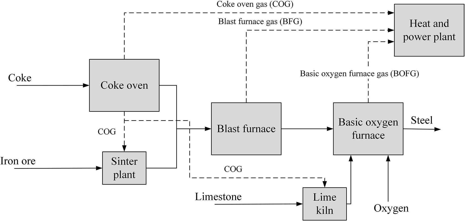
Figure 1. Diagram of an integrated steel mill, showing the main unit operations and where the three steel mill gases are produced. Adapted from Wiley et al. (2011).

TABLE 1

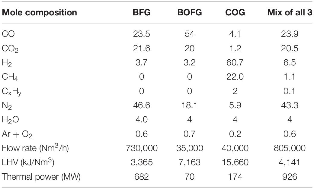
Table 1. Compositions and other key values for each steel mill gas for a modern steel mill producing 6 Mt of steel per year (Uribe-Soto et al., 2017).

Current Usages for Steel Mill Gases

As steel mill gases are only partially combusted, they provide energy for different usages in the plant. These can be clustered as follows, two of which provide useful energy and one for emergencies:

Electricity Generation

The steel mill gases are used to generate electricity or steam while being co-fired with natural gas or coal in a power plant. The electricity can be used on-site or sold to the electricity grid.

Heat Generation

The steel mill gases are burned in burners on-site for heat generation within the plant.

Flaring

In some emergency situations, such as a build-up in gas pressure or failure of equipment, the gas must be flared (Damodara, 2018). The flared gas is not useful in any way to the steel producer.

Most steel mill gases (73.3% when averaged across all three gases) are used for the generation of electricity, with the bulk of the rest being used for heating, although this differs from plant to plant. Often, the usage of the gases can be switched on short notice, particularly if they are being combusted in a combined heat and power plant (CHP). The amount of gas flared varies from around 0.1 vol% to 22 vol% (U.S. Department of Energy [DOE], 2010; Lundgren et al., 2013), with the average European steel plant flaring 2 vol% of their gas. Flare rates above 5 vol% typically only occur in modern plants where there is a failure or maintenance on one of the pipelines or power plant components. All three types of steel mill gas can be used for any of these purposes using a gas management system (U.S. Department of Energy [DOE], 2010; Lundgren et al., 2013; Sadlowski and Van Beek, 2020), although BFG is usually only used for heating in particular uses such as the coke plant or in combination with another fuel due to its lower flame temperature (Hou et al., 2011). The usage of the gas for either heating or electricity generation by the steel mill depends on factors unique to each steel mill, such as the presence of cold rolling or coating lines or the location of the coke oven within the plant (Carbon4PUR, 2020b).

Chemical Uses for Steel Mill Gases

The chemical industry currently depends significantly on fossil fuels for chemical production, leading to high carbon footprints (and fossil depletion) of chemical products. Due to the relatively high CO, CO₂, and H₂ content in steel mill gases, they are a potentially attractive alternative as a feedstock for the chemical industry. Desired molecules could be captured, or products could be produced directly from the gas, leading to an extensive range of possible chemical products (Stießel et al., 2018). Although there have been many studies on producing basic chemicals from pure CO₂ (Aresta, 2010; Quadrelli et al., 2011; Artz et al., 2018; Chauvy et al., 2019), there has been hardly any work focusing on using combinations of CO and CO₂ (as is present in BFG). If steel mill gases could be directly used, it could be economically beneficial as it would avoid expensive separation and purification of the gas. Both the CO and CO₂ present can be reacted with H₂ to produce valuable hydrocarbons. Economic assessments could then be performed to determine if the benefit from a purer feed stream outweighs the cost of separation for a particular process, as is the case in Carbon4PUR.

Many chemical syntheses from pure CO₂ are limited environmentally and economically due to the amount of H₂ required to produce products. For CO₂ utilization to be environmentally advantageous, this H₂ has to be provided by a low-emissions source (such as electrolysis based on renewable electricity), which is still comparatively expensive (6700 €/ton), despite efforts to reduce cost (Saur and Ramsden, 2011; Gielen et al., 2019; IEA, 2019). H₂ from COG could be captured using pressure swing adsorption and used for this purpose (Flores-Granobles and Saeys, 2020). A summary of some possible utilization options from steel mill gases is shown in Figure 2. It is estimated that the entire demand for methanol and ethanol in Europe could be met if 77% of the steel mill gases produced in Europe were used for chemical production (CORESYM, 2017).

FIGURE 2

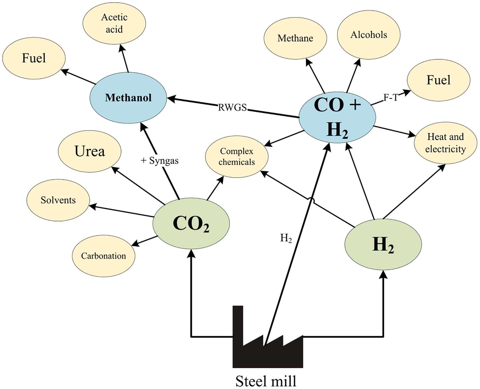
Figure 2. Summary of possible utilization options from steel mill gas adapted from Milani et al. (2015) and Hernández et al. (2017).

The largest barrier facing the utilization of steel mill gases for chemical production at the present is mostly the technological development of processes that are both economically and environmentally competitive with conventional processes. Other problems are logistical in nature, such as finding locations where chemical plants are in close proximity to steel mills, or who would take ownership of the chemical plant if a new one was to be constructed on the site of the steel mill. The Carbon4PUR consortium addresses these problems with specialized work packages (Carbon4PUR, 2020a).

Current Literature on Steel Mill Gas Valuation

Although there have been many techno-economic and life cycle assessments on the use of steel mill gases as a feedstock for chemical processes, most do not take into account any cost or GHG emissions for using steel mill gas as a feedstock, despite the gas providing energetic value to the steel mill. Ou et al. (2013) justify this by assuming that the steel mill gas used for their chemical process is gas that would otherwise have been flared; while this may be a valid assumption in China, where flaring rates are very high, this is not a valid assumption for a continuous process in Western Europe as the amount of flared gas ranges from 0.1 to 22 vol%, averaging around 2 vol% (Lundgren et al., 2013; Carbon4PUR, 2020b). Other studies do not provide any justification for their assumption of zero replacement cost or emissions (CORESYM, 2017; Deng and Adams, 2020). Those studies that do assume a purchase cost for steel mill gases usually assume a constant cost that may not accurately compensate the steel mill for the real value that steel mill gases provide for a given plant. Lundgren et al. (2013) assume a constant cost of 22.4 €/MWh for COG, while BFG and BOFG are assumed to be free. Yildirim et al. (2018) assume that COG will be replaced by natural gas within the plant, and the purchase cost of COG is effectively the cost of natural gas required to replace it. While this is an informed assumption, it neglects the other usages of steel mill gases (electricity generation and flaring) and how that varies dynamically, and again no purchase cost for BFG or BOFG is assumed. Lee et al. (2020) is the only study found to assume a purchase cost for BOFG as well as COG, using a static value for the cost of natural gas required to replace their energetic value. Likewise, the life cycle assessment conducted by Thonemann et al. (2018) assume natural gas replaces all steel mill gases consumed. No studies found have thus far considered replacing the electricity generated at the power plant, nor considered a dynamic model where the cost is based on the real-time steel mill gas usages and the prices of the utilities required to replace them. More accurate estimates for the cost of steel mill gas that fairly reflect the value it provides to the steel mill are beneficial to both the chemical and steel producer to ensure adequate compensation for the steel mill gas and to allow for more precise techno-economic and life cycle assessments on future technologies.

Goal and Scope

The main goal of the study is to investigate the economic cost and environmental implication of using steel mill gases as a chemical feedstock in order to assess its synergetic potential. As a first step, the value of the gases to the steel mill must be derived. The steel producer gains energy in the form of heat and electricity from burning the steel mill gases, which can be used on-site or sold to the grid. Knowing the value this gas generates is crucial in order to derive the cost the chemical producer must pay for the steel mill gases, which they aim to use as a substitute for other feedstocks to produce and sell chemicals. Secondly, to be considered as a potential feedstock by a chemical company, utilization of the steel mill gases has to be more economically and/or environmentally attractive than conventional feedstocks. The benchmarks for the study are discussed in detail in Benchmark Definition. The findings of this study could then be used as an input to further, more specific techno-economic and life-cycle assessments on a particular chemical process. Intermediate gas storage will also be considered and assessed for potential economic and environmental benefits. A storage tank could be implemented to increase the amounts of flare gas used, which would decrease the replacement cost and global warming impact. The scope of the study includes the steel mill gas usages, from the moment the gases are produced to their consumption for heat or power generation, as shown in Figure 3. Any chemical processes or gas processing, transport of the gases, separation, or treatment needed for such processes is not included in the scope of this study. The goal is to determine the value of the “feedstock stream” as shown in Figure 3 which also provides an indication of the purchase cost for the chemical producer, by using an estimate for the cost of replacing the energetic value the steel mill gas provides to the steel mill. The environmental analysis aims to then study the associated GHG emissions of the replacement.

FIGURE 3

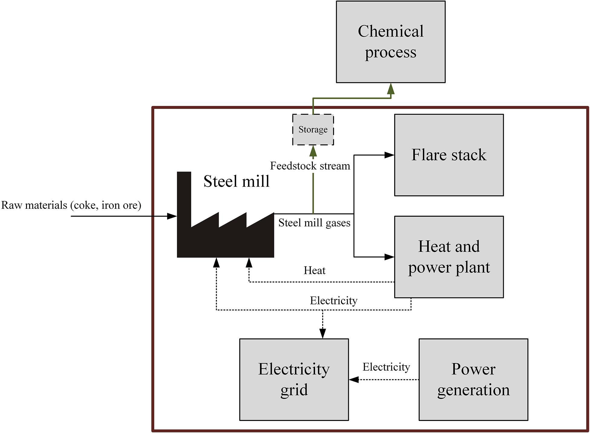
Figure 3. The scope of the study, including the usages of the steel mill gases and their replacements. Optional storage is shown in dashed lines.

Benchmark Definition

For the utilization of steel mill gases as a feedstock to become adopted, it must perform better than conventional feedstocks at whichever economic or environmental metrics are considered important by individual decision-makers. Benchmark feedstocks for steel mill gases are the base chemicals that are the most valuable components in each steel mill gas – CO for BFG and BOFG, and H₂ for COG. Although CO₂ is also a potentially valuable component of BFG and BOFG for CO₂ utilization processes, if it was desired as the only product, it could simply be taken from the waste steel mill gases after combustion in the CHP at a higher concentration. Therefore, it will only be considered as a “secondary” feedstock or benchmark, useful in such processes that are designed to use both CO and CO₂. However, although CO₂ is more likely to be used as an additional feedstock than the main one, if it is used in a process alongside CO, such as the Carbon4PUR process, knowing the replacement cost is valuable information.

The benchmark for CO is defined to be CO produced from fossil fuels through coal gasification, which has production costs of around 440 €/ton (Pei et al., 2016) and a GHG emissions impact of approximately 1.25 kg-CO₂-eq./kg CO (Wernet et al., 2016) for a cradle-to-gate system boundary.

For H₂, two benchmarks are defined: firstly, a steam reforming process, representing conventional, fossil-based H₂ production, and a solar-powered electrolyzer process, representing an alternative non-fossil-based production method. The steam reforming process has production costs of around 2200 €/ton, and the electrolysis method currently around 6700 €/ton (Gielen et al., 2019). Steam reforming has a GHG emissions impact of 4.8 kg-CO₂-eq./kg H₂ (Dufour et al., 2011) and solar-powered electrolysis of around 2.0 kg-CO₂-eq./kg H₂ (Bhandari et al., 2014) when taking into account cradle-to-gate emissions.

As well as a comparison to conventional benchmark feedstocks, from an environmental perspective, usage of steel mill gases should reduce overall emissions from the system, i.e., replacing the heat and electricity to the steel mill should not generate more emissions than the steel mill gases otherwise would have. Therefore, the emissions results from this study are also compared to a “viability point,” above which emissions are no longer saved when steel mill gases are used.

Scenario Definition

The base scenario is defined as a mid-flaring, mid-capacity steel mill in the year 2017 in France using BFG. Variables that are altered and compared are done so from this base scenario. For example, if differing capacities are being compared, they are done so at a mid-flaring level in 2017. In most cases, both countries studied are also compared directly.

Germany and France are selected as the studied countries because they are both large economies with substantial chemical and steel industry (Statista, 2020), as well as containing particular locations where such a symbiosis could take place (Fos sur Mer in France, Ruhrgebiet in Germany). There is a large difference in how electricity is produced for the grid in each country, making both economic and environmental comparisons interesting. France’s electricity grid has one of the lowest GHG emissions intensities in Western Europe, while Germany has one of the highest, making it possible to see results for both “best” and “worst” case scenarios.

The gas feedstock capacities are selected based on appropriate amounts required for example processes, as mentioned in the list below. The maximum capacity for BOFG and COG is around 400 and 250 kt/a, respectively, and therefore that was the upper limit that was simulated for them. The average flare rate in European steel mills is around 2 vol%, and this was consequently chosen as the value for the base scenario. Boundaries as low as 0.5 vol% and as high as 5 vol% were also simulated to ensure the limits of most modern steel mills are covered.

All three types of steel mill gas are considered in this study. For smaller chemical syntheses, solely BOFG or COG could be used for the feedstock, but using BFG is required for larger plant capacities. It is believed that most steel mill flue gas utilization processes will focus on solely using BFG, as it accounts for roughly 85% of the emitted steel mill gases. However, some processes utilizing multiple gas streams are under research, such as the production of syngas by mixing BFG and COG (Lundgren et al., 2013).

The year 2017 is chosen as the base year of the study as initial research was started this year; neither grid prices nor emissions factors have significantly altered since then. As a future scenario, the year 2050 is selected due to the relative abundance of data available for grid emissions predictions for this time; as well as this, many countries and industries have set specific emissions-related goals for 2050. Forecasts predict that the majority of steel produced in 2050 will still be by the integrated steel mill route and that steel mill gas utilization will be required to meet 2050 emissions targets (EUROFER, 2019). This scenario only analyses GHG emissions; utility price predictions 30 years in the future are too uncertain to be used.

In summary, the following possibilities for each variable were thereby derived:

Location:

• France.

• Germany.

Gas capacity:

• Low capacity – 25 kt/a – Very small industrial plant (e.g., specialty chemicals such as rubbers).

• Mid capacity – 100 kt/a – Medium-sized industrial plant (e.g., common polymers, intermediate chemicals such as polyethylene).

• High capacity – the highest feasible scale of gas usage (BFG: 1000 kt/a or BOFG: 400 kt/a or COG: 250 kt/a) – very large industrial plant (e.g., large scale base chemicals such as methanol) (different plant sizes here are due to the three gases having different quantities).

Type of steel mill gas used as feedstock:

• BFG – Used for most flue gas utilization processes studied thus far due to very large capacity.

• BOFG – Useful if gas is desired with slightly higher carbon content than BFG.

• COG – Useful if H₂ or CH₄ is desired.

Mill flaring rates:

• Low flaring – 0.5 vol% – more likely in modern plants.

• Mid flaring – 2 vol% – average flaring rate for European steel mills.

• High flaring – 5 vol% – could happen in circumstances with ongoing maintenance or broken parts in the power plant or heat generation systems.

Year:

• 2017 – Reflecting present time grid emissions intensity.

• 2050 – Reflecting future grid emissions intensity (from ecoinvent 3.6, 450 2050 scenario).

Any of these variables can be changed to create a multitude of possible unique scenarios, one “branch” of which is demonstrated in Figure 4.

FIGURE 4

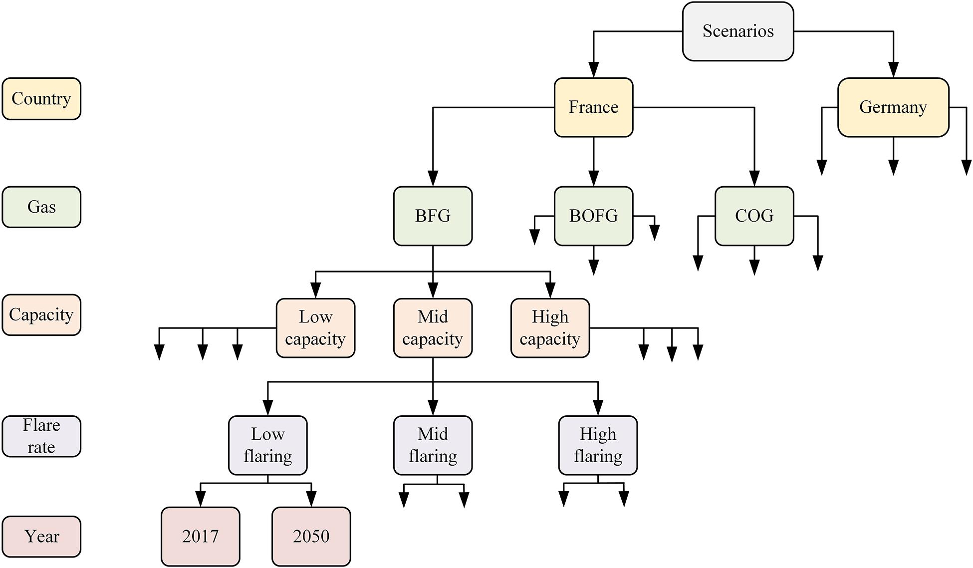
Figure 4. Tree diagram of the different scenarios possible by changing model parameters. Only one “branch” is shown for diagram simplicity.

Data Collection and Manipulation

Data Collection and Assumptions

Data were obtained from a major steel producer from two of their steel mills detailing how much gas is used for electricity generation, heating, or is flared. One of the datasets covers a representative 2-month period on a 10 min basis, while the other has measurements on an hourly basis over a complete year. One of these mills (hereafter referred to as the “non-efficient case”) had a particularly high flaring rate due to technical issues (one of the highest flaring rates in Western Europe), and the other (“efficient case”) had one of the lowest flaring rates in Western Europe.

The spot market prices for both electricity and natural gas in both Germany and France were obtained for the year 2017. It is assumed that these prices have not greatly varied since 2017 and that the random fluctuations present in the price are of the order of magnitude that can also be found in previous or later years.

The greenhouse gas emissions are calculated using LCA data on global warming impact from ecoinvent 3.6 (cut-off system model) [tons-CO₂-eq,/kWh] (Wernet et al., 2016). The share of electricity generated in Germany and France from each source type (coal, wind, etc.) was found for every hour over the year 2017 (Bundesministerium für Umwelt, 2020; ENTSOE, 2020; Fraunhofer, 2020; RTE, 2020; Umweltbundesamt, 2020). For the scenarios set in 2050, data for the predicted carbon intensity of the grid, again in [tons-CO₂-eq,/kWh], was also obtained from ecoinvent 3.6 (Stehfest et al., 2014; Mendoza Beltran et al., 2020).

It is important to note that the power plant and burner efficiency has an impact on the value the gas provides for electricity generation or heating purposes (Worrell et al., 2010). The power plants in steel mills have efficiencies that vary from 0.3 to 0.5 (Kim and Lee, 2018). An efficiency of 0.36 is commonly used in literature (Harvey et al., 1995; Kim and Lee, 2018), and the same value was chosen for this study after discussion with a steel manufacturer. Higher efficiencies mean that more electricity or heat can be generated for a certain amount of steel mill gases in the power plants, resulting in the steel mill gases being more valuable.

Simulation of Steel Mill Flaring Data

From the flaring patterns in the data obtained from the steel mill, a flaring pattern for an average Western European steel mill is simulated. As the “non-efficient case” has a very atypical flaring pattern due to technical issues, the simulation for the study was based on the patterns in the data set from the “efficient case.” It is assumed that the flaring pattern for the average case would look similar to the efficient case but simply scaled up.

A discrete-time Markov chain is implemented to simulate flaring patterns across a range of potential steel plants (Mcbratney and Everitt, 2002; Towers, 2016; Gagniuc, 2017). Three Markov transition matrices are created from the amount of gas being flared every hour, wherein the first bin of the first matrix contains the second Markov transition matrix, and likewise with the second to the third, as illustrated in Figure 5. With this method, both appropriate resolution and probability of flaring events are retained from the original data. Two variables are considered to be critical to the replication of realistic flaring data: the frequency of times when flaring is zero and the overall average volume of gases flared (essentially equal to flaring rate). Realistic ranges for these variables were created using linear regression from the data provided by the steel manufacturer for multiple steel mills. The heat maps of the Markov transition matrices highlight the moderate probability of a given flaring amount maintaining a similar amount into the next hour, as well as the high likelihood of a flaring event going to zero. Flaring events usually last a few hours or days and do not change between non-zero values too erratically.

FIGURE 5

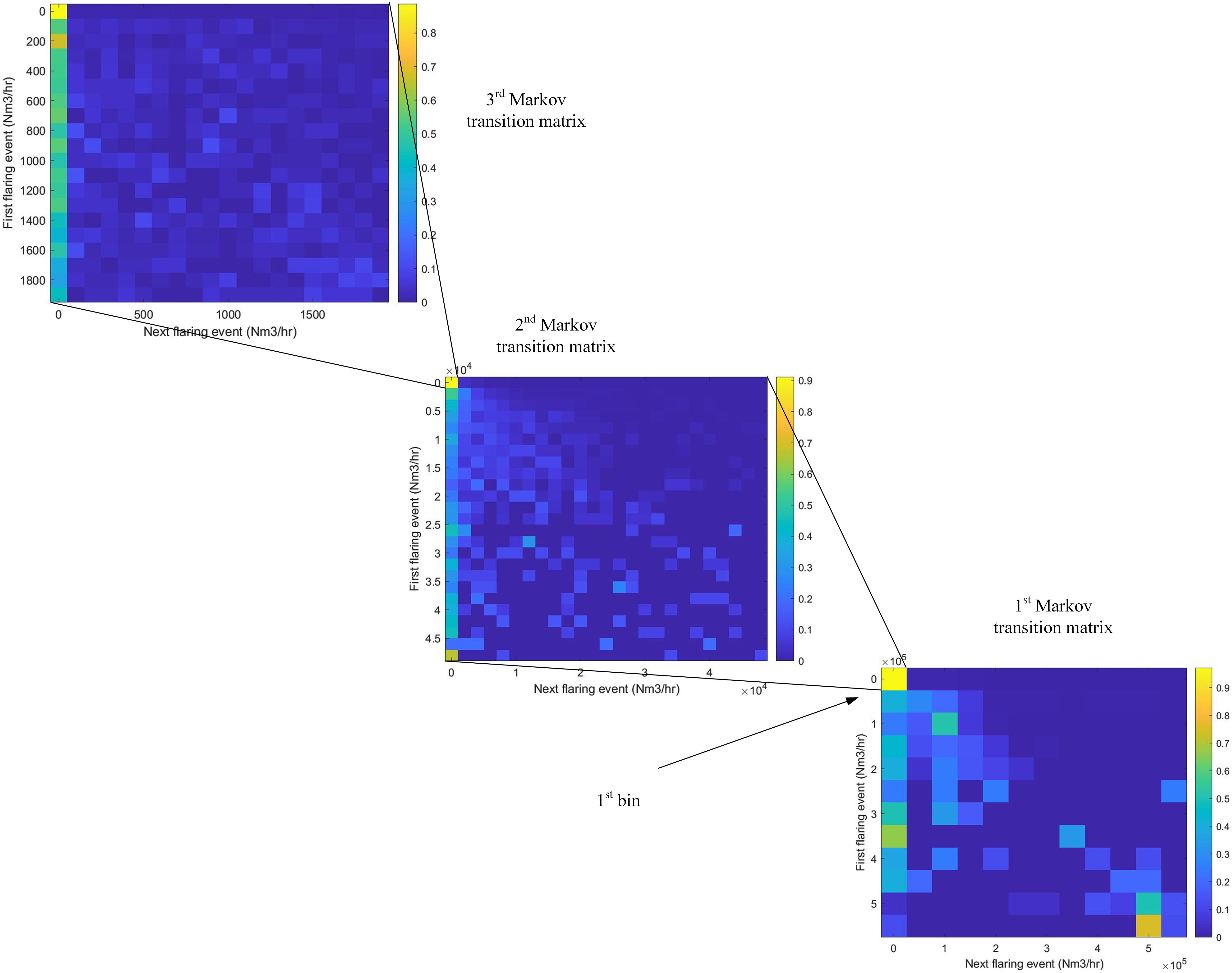
Figure 5. Heat map of the Markov transition matrices, indicating probability of the flaring amount (Nm³) at the next hour given the amount at the current hour. The first bin of the first Markov transition matrix leads to the second transition matrix, and vice versa for the second to third. Data is shown here for a 2% average flare rate steel mill.

Model Description

Modeling the Replacement Cost of Steel Mill Gases

The economic value of the steel mill gases depends directly on the economic value that it supplies to the steel producer. This economic value is entirely based on the energy gained from the combustion of the gas. As mentioned in Current Usages of Steel Mill Gas, the steel mill gases are either combusted for electricity generation, heat, or are flared. Each of these options provides a different economic value. Essentially, the steel mill gases’ economic value can be viewed as the cost to replace these usages by another source. For example, if steel mill gases that would otherwise have been used to generate electricity were instead used as a chemical feedstock, the electricity that would have been generated needs to be replaced by another source. This electricity could either be purchased from the local grid or generated on-site by other means. Likewise, for heating, the heat that would have been generated by steel mill gas that is now used instead as a chemical feedstock could be generated instead by natural gas or other means.

A single-objective cost-minimization model was created in the programming platform MATLAB that follows the following logic tree shown in Figure 6. The model is run according to a logical hierarchy: first, if there is enough gas being flared at a particular moment to supply the feedstock demands for a specific chemical plant, then the gas could be obtained effectively at zero cost by the chemical producer. Second, when there is not enough flare gas to meet demand, the electricity gas is taken next, which is replaced by either buying electricity from the grid or generating that electricity with natural gas directly. Third, when there is not enough electricity gas or flaring gas to meet the demand, heating gas is chosen, and natural gas is burned to replace heat that would otherwise have been generated by the steel mill gases. The model allows for varying the plant capacity (and therefore the amount of steel mill gases used), the input dataset from the steel mill (or another industrial plant), the electricity and natural gas prices, the efficiency of the steel mill, the flaring rate in volume and the frequency of flaring of the steel mill.

FIGURE 6

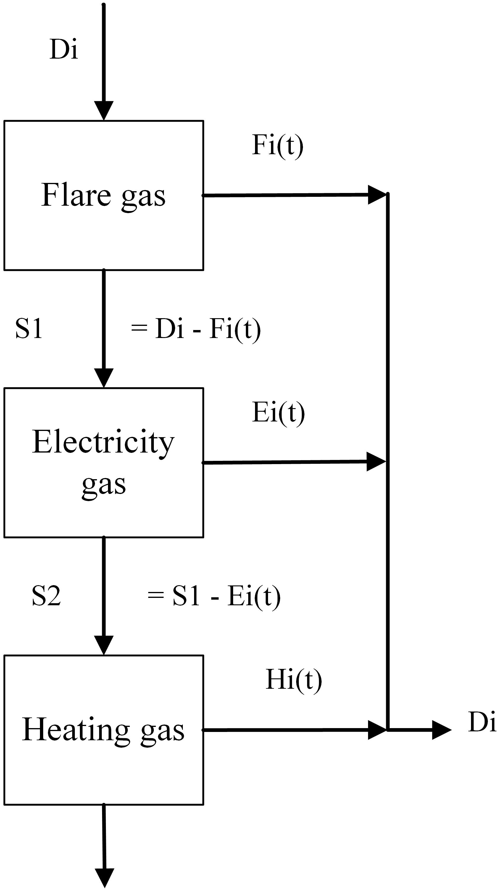
Figure 6. The three different potential usages of steel mill gases and how the amount of each one is decided. F_i(t), E_i(t), and H_i(t) are the amounts of steel mill gas that are taken from flaring, electricity production and heating, respectively. D_i is the total gas demand. S₁ is the amount of gas that cannot be met by flared gas, and S₂ is the amount that cannot be met by flaring or electricity gas.

The most desirable steel mill gases to take for chemical feedstocks are gases that would have otherwise been flared (hereafter referred to as “flare gas”). In flaring, no energy is recovered, so no value can be gained. Regarding costs, most flare stacks are usually required to constantly burn a natural gas ignition flame, meaning that operating costs are not expected to differ noticeably during periods where gas is flared or not (Damodara, 2018). As flaring provides no economic benefit or value to the steel producer, the replacement cost of flaring gas (RC_flare) is zero, independent of time:

$$R{C}_{flare}=0$$

Consequently, for the chemical producer, the gas is essentially free from a material cost basis (capital infrastructure and transport costs are discussed in section “Estimation of Storage Potential”) and is the top priority for feedstock gas.

Feedstock gas that would otherwise be used for electricity generation (hereafter referred to as “electricity gas”) does provide economic value to the steel producer. Another source must replace this electricity (or at least the economic value it provides). In this study, two sources are considered: purchasing electricity from the grid, and producing electricity directly from natural gas. Natural gas is already co-fired with BFG in many power plants due to the comparatively low energetic value of BFG. Therefore, this process does not require any extra process units nor incur higher operating costs outside of the cost of natural gas. Steel mills have a gas management system that allows for the usage of the gas to be altered on short notice. The replacement cost of electricity gas (RC_electricity at a particular time (t) is the cheaper of the two alternatives at that time:

$$R{C}_{electricity}(t)=\text{min}[R{C}_E(t),R{C}_{NG}(t)]$$

It might also be the case that the steel mill would not buy energy directly from the grid if that is the cheapest option, as electricity is usually produced in excess by the steel mill and sold to the grid. The chemical company would simply then reimburse the lost revenue of the steel company, which is essentially the price of that amount of electricity from the grid at that time.

Feedstock gas that would be otherwise used for heating (hereafter referred to as heating gas) can only be easily replaced by natural gas. Burners in a steel mill already have natural gas present to co-fire with steel mill gases when required, so that the mill can maintain production in the case of a lack of steel mill gases due to maintenance or failure in the gas distribution system. Therefore, the replacement cost of heating gas (RC_heating) at a particular time (t) is equal to the natural gas price at that time:

$$R{C}_{heating}(t)=R{C}_{NG}(t)$$

Note that this does not mean that the same volume of natural gas has to be purchased as that of the steel mill gases that were taken for feedstock; only the amount of natural gas that replaces the energetic value that the steel mill gases would have provided.

To calculate the overall replacement cost (RC_T), the amount of steel mill gas taken from each source is multiplied by the cost to replace it for each source. For detailed calculations on how the replacement costs are calculated, refer to the Supplementary Material section “Calculations for the Choice of Steel Mill Gas Source.” It is assumed that the steel mill can change between these options on an hourly basis, based on the fact that they can burn natural gas in the burners currently with little planning (Sadlowski and Van Beek, 2020).

Estimation of the GHG Emissions of Steel Mill Gases Usage

To assess the global warming impact of steel mill gas utilization, the GHG emissions of the dynamic stream determined by the cost-minimization model in Modeling the Replacement Cost of Steel Mill Gases must be calculated. For the year 2017, if electricity from the grid is used to replace the electricity generation of the steel mill gases, the amount of grid electricity that is required at a given hour [E_R(t)] is multiplied by the share of each gas (x_i) and the emissions intensity data for the respective source (EI_i) from ecoinvent, giving a total amount of GHG emissions for that hour from electricity [GHG_E,17(t)] in the unit of [tons-CO₂-eq.]:

$$GH{G}_{ET,17}(t)=E_R(t)\sum _i{x}_i(t)E{I}_i$$

If natural gas is used, either to replace electricity or for heating, the GHG emissions for that hour from natural gas [GHG_NG,17(t)] are determined by multiplying the amount of natural gas required [NG_R(t)] by the emissions factor for natural gas (EI_NG).

$$GH{G}_{NG,17}(t)=N{G}_R(t)E{I}_{NG}$$

The total GHG emissions for a given hour [GHG_T,17(t)] is then the sum of both the GHG emissions from electricity and those from natural gas:

$$GH{G}_{T,17}(t)=GH{G}_{NG,17}(t)+GH{G}_{E,17}(t)$$

For the year 2050, it is assumed that grid electricity would be cheaper to use than natural gas to replace electricity generated by steel mill gases due to carbon taxes and renewable energy development. Therefore, only grid electricity is used to replace electricity generated by the steel mill gases. This amount of electricity required to replace the electricity generation of the used steel mill gases [E_R(t)] is multiplied by the carbon intensity of the grid (EI_G) to give the total GHG emissions for that hour [GHG_T,50(t)] in [tons-CO₂-eq.].

$$\begin{array}{c}\\ GH{G}_{T,50}(t)=E_R(t)E{I}_G\hfill \end{array}$$

It should be noted that in the year 2050 it is unclear if heating in the steel mill will still be conducted by natural gas or if it will be replaced by lower-emission forms of heating. Some of the solutions currently being investigated include using bio-methane or biomass, H₂ that is produced from BFG for specially developed burners, inductive heating from steel strips for coating, or simply capturing and storing the emitted CO₂ from heating with natural gas (Carbon4PUR, 2020b). However, these technologies are at a low technology readiness level and require further development. Due to the very different and unknown costs and emissions associated with each of these, as well as the uncertainty of which technology is the most likely to become widely adopted, these possibilities are not considered in this analysis. Therefore, GHG emissions for the 2050 scenario could be considered as a conservative estimate; emissions from steel mill heating will likely be reduced in some capacity by the year 2050.

It is assumed that the emissions from the rest of the value chain outside of the scope of the study remain constant and do not change between a scenario where steel mill gases are used for chemical production and one where no steel mill gases are used (for example, that the same amount of steel is produced, and the same amount of coal is required). In this case, the emissions determined in this study can be directly compared to the cradle-to-gate emissions of the benchmarks. As the emissions required to produce the steel do not change, the only emissions that can be allocated to steel mill gases as a feedstock are those emissions required to replace the usage of the steel mill gases. The end “gate” of the study is the same point as the benchmarks, which is when a ready feedstock is produced. The steel will be produced with or without steel mill gas utilization, and therefore all other and previous emissions are allocated to the steel production itself, which is the main product of a steel mill.

Estimation of Storage Potential

If gas storage is to be used, it should be optimally sized for the given gas capacity. If the storage is too large or small, the capital investment required might outweigh the savings gained by reducing steel mill gas replacement costs. The storage size was an alterable variable in the model, and if gas was flared, it was taken into the storage until the storage was either full or there was no more flare gas to be used. At this point, electricity gas was taken into storage, and finally heating gas if no more electricity gas was available. This ensures a much higher ratio of flare gas is used and therefore lowers both cost and emissions required to replace the steel mill gases. The cost of the storage tank was determined as follows (Sinnott and Towler, 2009), with a general empirical formula for equipment cost of unit operations.

$$C_e=a+b{S}^{n}in[\frac{\text{C}\text{=}}{a}]$$

Where a = 97,000, b = 2,800, n = 0.65, and S = size in m³ between 100 and 10,000 m³.

The size was then varied to find the optimum storage size for a particular steel mill. This optimum was found at the lowest total cost when the annualized equipment cost for the storage was added to the cost per year of steel mill gas. The investment cost was then annualized (Chiuta et al., 2016):

$$annualizedCapEx=CapEx\frac{i}{1-{\left(1+i\right)}^{-L}}\mathit{\hspace{1em}}in[\frac{\text{C}\text{=}}{a}]$$

Results

Replacement Costs From an Energy Perspective

This section discusses the average replacement costs in 2017 Euros from an energy perspective by former usage options across the year 2017; results are shown in Table 2. Both the type of gas chosen and its usage have drastic impacts on the economic value it provides to the steel mill, and therefore also on its replacement cost. BFG has a relatively low replacement cost for both power generation (15 €/ton in France) and heating (21 €/ton in France). BOFG has a higher calorific value due to its higher CO content, resulting in a replacement cost of 52 €/ton for electricity generation. COG has the highest calorific value as a result of the large H₂ and CH₄ content and therefore has also the highest replacement cost (205 €/ton for electricity generation in France).

TABLE 2

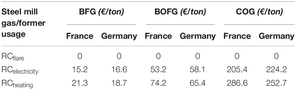
Table 2. Average replacement costs over the year 2017 for the different steel mill gases and respective usages.

Gases used for heating also have about 40% higher replacement costs than gases used for electricity generation on average, due to the higher costs of natural gas. Therefore, it will usually be more beneficial to take feedstock gas from the stream to the power plant than the stream used for heating. Germany has a higher replacement cost for electricity generation (about 5%) in all three gases, and likewise lower for heating (14%), which directly results from the difference in prices for electricity and natural gas between the two countries.

Figure 7 details which gases are most frequently used for which purpose in vol%. BFG is flared the most at 20%, while COG and BOFG are flared at around 5%. Non-flared BFG is almost exclusively used in the power plant, while COG is used only for heating. BOFG is spread more evenly, with a 68% share used in the power plant and 25% used for heating. The higher flared volume in BFG is a positive indication that BFG is likely to perform better economically and have a lower global warming impact than the other gases.

FIGURE 7

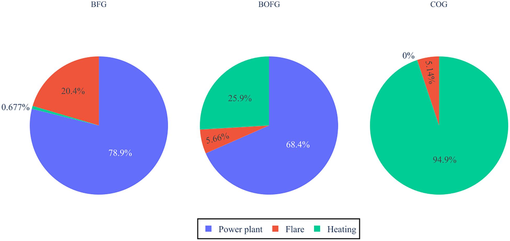
Figure 7. Usages of each steel mill gas for the baseline system if they would have been used in the steel mill conventionally.

Replacement Costs From a Chemical Feedstock Perspective

This section discusses the costs from a feedstock perspective; the analysis assumes that the respective steel mill gases are used as feedstocks in the chemical industry for a CO and CO₂ mix (A), and CO (B), CO₂ (C), and H₂ (D). Results are shown for each capacity scenario in Figure 8. For example, when BOFG serves as a feedstock for CO and CO₂ in France at high capacity, the steel mill has to cover replacement costs of 70 €/ton. COG is not shown in subplots B and C because it contains very minor amounts of CO and CO₂; likewise, BFG and BOFG only contain small amounts of H₂ and are therefore omitted from subplot D.

FIGURE 8

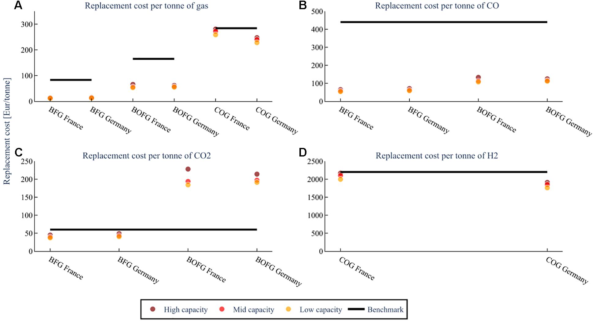
Figure 8. The replacement cost of the steel mill gases when using them as chemical feedstocks for different capacity scenarios; low capacity (25 kt), mid capacity (100 kt), high capacity (1000 kt/a BFG or 400 kt BOFG or 250 kt COG, at a flare rate of 2%. The costs for (A) assume both CO and CO₂ are used. The costs for (B–D) are assuming that feedstock is the only one used. The benchmark is the cost of the feedstock when produced from conventional sources.

Subfigure A assumes that the steel mill gases are used as feedstocks for both CO and CO₂. In this case, both replacement costs for BFG (11–15 €/ton) and BOFG (52–65 €/ton) are considerably lower than their benchmarks (83 and 165 €/ton, respectively). Although BOFG has only a slightly higher CO content than BFG, the fact that it is flared much less (5% compared to 20% by volume) results in a significantly higher gas price. The replacement costs for COG are just slightly lower than the benchmark (284 €/ton) for France (258–280 €/ton) and about 15–20% lower for Germany (227–247 €/ton). These results are a positive indication that BFG and BOFG are economically viable when both CO and CO₂ are utilized.

In subfigure B, it is assumed that the steel mill gases are used as feedstocks for CO only. Compared to the benchmark (440 €/ton), the replacement costs of both BFG (50–70 €/ton) and BOFG (100–130 €/ton) are significantly lower, which is a positive indication that usage of CO from steel mill gases is more economically favorable than conventional CO for all scenarios. Usage of BFG and BOFG for CO is especially interesting for chemical processes that do not require a pure CO stream.

In subfigure C, it is assumed that the steel mill gases are used as feedstocks for CO₂ only. The costs for CO₂ from BFG are 37–48 €/ton, which is lower than the benchmark (60 €/ton). For BOFG, however, the costs are significantly higher (184–228 €/ton). Using CO₂ from BFG is therefore economically viable, even if CO were also not used. It is not recommended to use BOFG to obtain CO₂ as a feedstock.

In subfigure D, it is assumed that COG is used as feedstocks for H₂ only. The replacement costs for H₂ for the base scenario are about 2100 €/ton, varying from 2168 €/ton for 250 kt/a COG to 1877 €/ton for 25 kt/a COG. This is also on par or slightly less than the benchmark’s price, conventionally produced H₂ from steam reforming (2200 €/ton) (Gielen et al., 2019). Therefore, usage of H₂ from COG could be economically feasible for a small or medium-sized chemical process plant. It is important to note that H₂ separation costs should be added if the H₂ is desired pure.

The replacement costs were also calculated with the different flaring scenarios; however, different flare rates have a smaller impact on the replacement cost of the steel mill gases than different capacities [see the Supplementary Material Section “Results for Differing Flare Rate Scenarios”]. The viability compared to benchmarks for the flaring scenarios are similar to that described above for the capacity scenarios. It should be noted that all replacement costs mentioned here do not include separation or purification of the feedstock, transport, or additional costs imposed by the steel producer.

Replacement Greenhouse Gas Emissions From a Chemical Feedstock Perspective in 2017

The amount of GHG emissions (tons-CO₂-eq.) required to replace the steel mill gases used is shown in Figure 9 for the three capacity scenarios for a CO and CO₂ mix (A), and CO (B), CO₂ (C), and H₂ (D). For example, the number of emissions required to replace the electricity and heat that a high capacity BOFG scenario in France is about 0.75 tons-CO₂-eq/ton of BOFG.

FIGURE 9

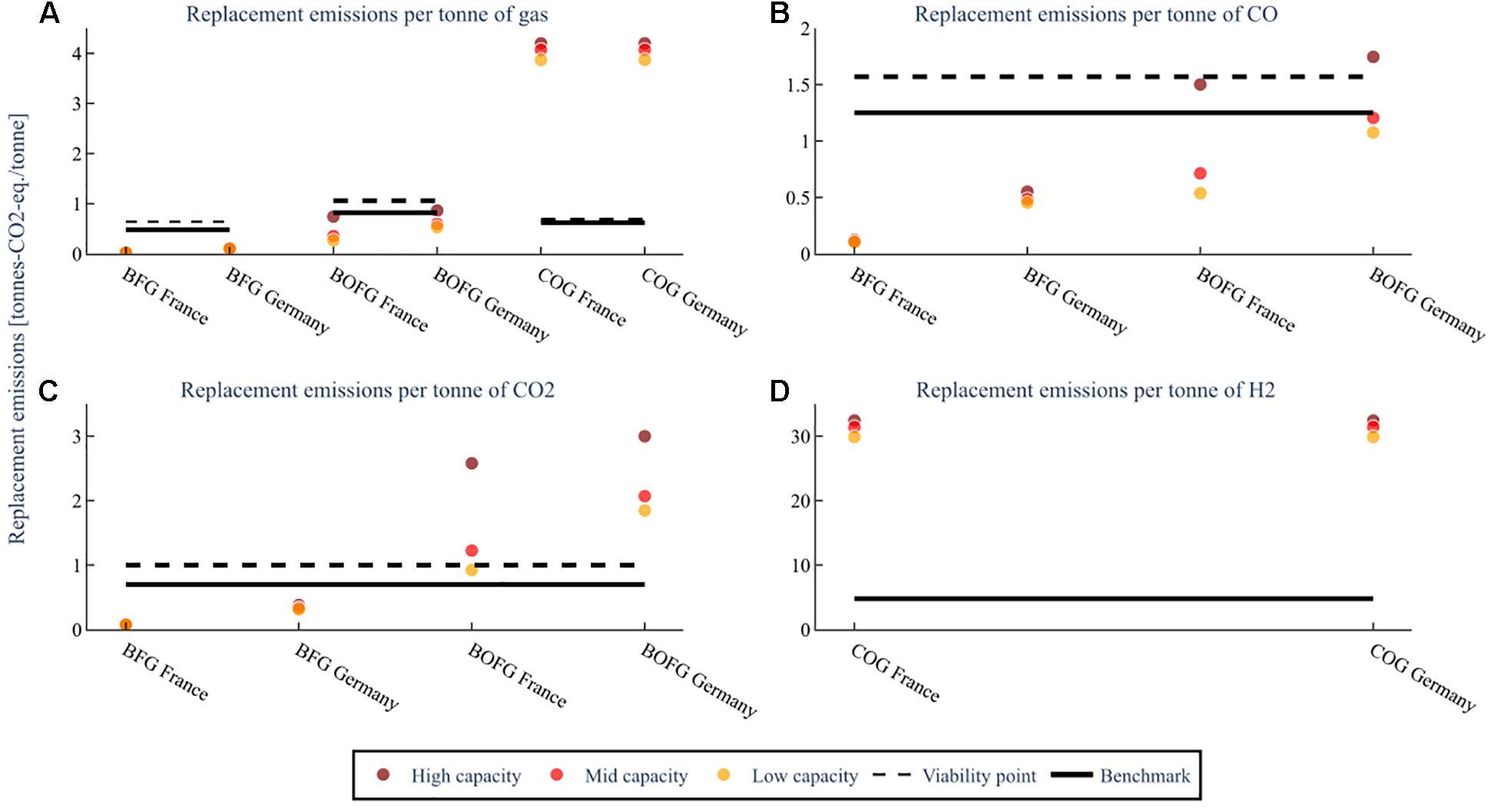
Figure 9. The GHG emissions required to replace the energy provided to the steel mill by the steel mill gases for the three capacity scenarios; low capacity (25 kt), mid capacity (100 kt), high capacity (1000 kt/a BFG or 400 kt BOFG or 250 kt COG), at a flare rate of 2%. The replacement emissions for (A) assume both CO and CO₂ are used. The replacement emissions for (B–D) are assuming that feedstock is the only one used. The benchmark is the global warming impact of the feedstock when produced from conventional sources.

If both CO₂ and CO are used, as is effectively shown in subfigure A, then the viability point for BFG (0.64 tons-CO₂-eq/ton BFG) and BOFG (1.06 tons-CO₂-eq/ton BOFG) are both well above the replacement emissions (0.02–0.11 tons-CO₂-eq/ton BFG and 0.26–0.84 tons-CO₂-eq/ton BOFG) required. Their use is therefore viable from an emissions standpoint. However, in all scenarios, BFG requires fewer emissions than BOFG and France less than Germany. BFG also clearly has much fewer emissions than the benchmark (0.64 tons-CO₂-eq/ton BFG and 0.82 tons-CO₂-eq/ton BOFG). In comparison, BOFG has fewer emissions for all scenarios in France and the lower and mid-capacity scenarios in Germany. COG has much higher emissions (3.9–4.2 tons-CO₂-eq/ton COG) than both the viability point and the benchmark for all capacity scenarios and countries.

For both countries, when using BFG (about 0.1 tons-CO₂-eq./ton CO for France and 0.43–0.55 tons-CO₂-eq./ton CO for Germany), the replacement emissions required per ton of CO (shown for BFG and BOFG in subfigure B) are lower than for the benchmark method of obtaining CO [1.25 tons-CO₂-eq./ton CO (Wernet et al., 2016)]. Also, for the low and mid-capacity scenarios for BOFG when located in France (0.53–0.71 tons-CO₂-eq./ton CO) and Germany (1.07–1.20 tons-CO₂-eq./ton CO), the emissions required to replace the steel mill gases are lower than the benchmark. However, for the high capacity scenario located in France (1.5 tons-CO₂-eq./ton CO) or Germany (1.75 tons-CO₂-eq./ton CO), the emissions required are higher than the benchmark.

For CO₂ (shown for BFG and BOFG in subfigure C), only the usage of BFG is lower than conventional methods [0.75 tons-CO₂-eq./ton CO₂ (Wernet et al., 2016)]. It should be noted that in the event of CO₂-only usage, replacement emissions of more than one ton-CO₂-eq./ton CO₂ means that the use of this CO₂ is not viable from the standpoint of reducing GHG emissions. This shows that while BFG is viable in both Germany and France, BOFG is only viable in France and then only at smaller to medium-sized plants.

The replacement emissions required per ton of H₂ (subfigure D) are extraordinarily high, around 31 tons-CO₂-eq. per ton of H₂ obtained, and the overall usage of H₂ results in emissions of around 27 tons-CO₂-eq. per ton of H₂ even when the emissions saved from avoiding combustion are taken into account. As even H₂ produced from conventional methods has a much lower emissions intensity ranging from 1.6 tons-CO₂-eq. per ton of H₂ for coal gasification (Wernet et al., 2016) to 4.8 tons-CO₂-eq. per ton of H₂ for steam reforming (Dufour et al., 2011), it is not recommended to use COG to obtain H₂ from a GHG emissions perspective.

The simulation for the different flaring scenarios (0.5–5% for BFG and BOFG, and 0.5–2% for COG) instead of capacities is shown in the Supplementary Material section “Results for Differing Flare Rate Scenarios,” Figure 4). As with the replacement cost, changes in the flare rate do not have as large an impact as changes to the plant’s capacity.

Replacement Greenhouse Gas Emissions From a Chemical Feedstock Perspective in 2050

It is important to consider that electricity grid mixes in the future could be vastly different from current grid mixes. Therefore, the same simulations for GHG emissions were completed with the predicted grid emissions intensity for the year 2050 in order to estimate the replacement emissions. The results are shown in Figure 10.

FIGURE 10

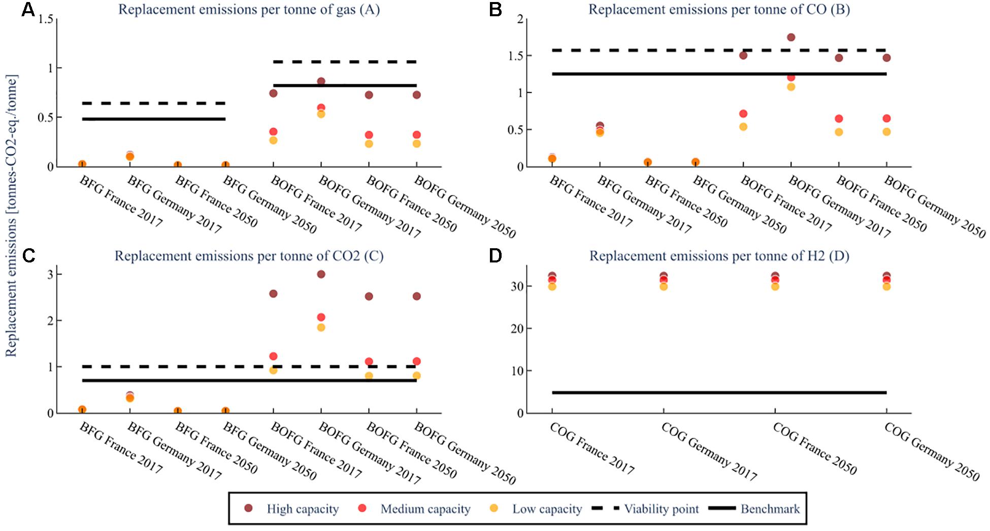
Figure 10. The GHG emissions required to replace the energy provided to the steel mill by the steel mill gases for the three capacity scenarios in 2050; low capacity (25 kt), mid capacity (100 kt), high capacity (1000 kt/a BFG or 400 kt BOFG or 250 kt COG), at a flare rate of 2%. The replacement emissions for (A) assume both CO and CO₂ are used. The replacement emissions for (B–D) are assuming that feedstock is the only one used. The benchmark is the global warming impact of the feedstock when produced from conventional sources.

In the 2050 scenario, a large decrease in the replacement emissions is seen for Germany for all scenarios, but for France, only a very slight decrease is observed due to the already low emissions intensity of the electricity grid in France. Both Germany and France are predicted to have similarly low grid emissions intensities by 2050 (<0.1 tons-CO₂-eq./MWh) (Wernet et al., 2016). The plot for the various flaring scenarios is shown in the Supplementary Material section “Results for Differing Flare Rate Scenarios,” Figure 5).

Replacement Costs and Greenhouse Gas Emissions When Gas Storage Is Used

A time-series plot of the replacement cost over the year 2017 for both Germany and France is shown in Figure 11. The replacement cost fluctuates quite significantly both on longer timescales throughout the year as a result of the electricity and natural gas prices, but also on much shorter timescales (days or hours) due to the steel mill gas usages (particularly the flaring volume, which often drives the replacement cost to zero). It could thus be beneficial to build gas storage, which could be filled when lower-valued flare gas is being drawn from the steel mill, and used up when there is no flaring and higher value electricity or heating gas is being drawn, taking advantage of these short-term fluctuations.

FIGURE 11

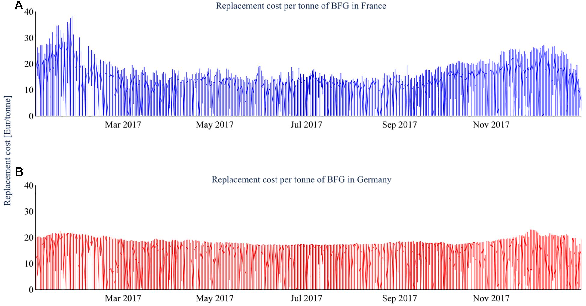
Figure 11. Time-series plot of replacement cost over the year 2017 for the base scenario (flare rate 2%, capacity 100 kt BFG) for both France (A) and Germany (B).

The capital cost of the storage was taken into account using commonly used capital cost estimation equations for a storage tank, based on the capacity of the storage (Sinnott and Towler, 2009). Storage size was plotted against annualized capital cost, yearly feedstock cost of the steel mill gas, and the sum of the two to find the minimum of this sum, which is the optimal storage size from an economic perspective and is shown in Figure 12.

FIGURE 12

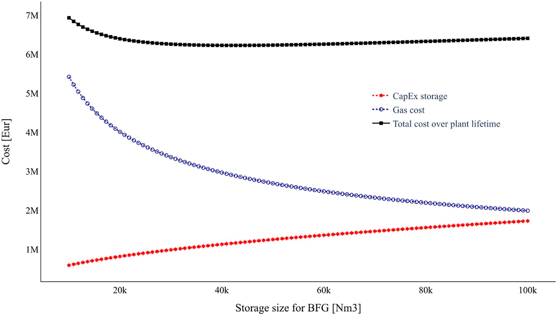
Figure 12. Optimization of storage size for the base scenario (flare rate 2%, capacity 100 kt BFG).

The optimum storage size for the base scenario was compared to the base scenario in Germany without storage. A comparison of the replacement cost is shown in Figure 13. For example, without storage, BFG has a replacement cost of about 13 €/ton. When the optimally sized storage is used, it drops to about 6 €/ton. A similar result can be seen when looking at the GHG emissions for the same scenarios in Figure 14, with even more significantly reduced GHG emissions for BFG and only a slight reduction for BOFG. The results show that optimally sized storage is advantageous for reducing both the replacement cost and GHG emissions impact of BFG by around 50% and is therefore recommended for BFG. On the other hand, negligible cost differences are seen for BOFG and COG, and therefore storage is not recommended for BOFG or COG.

FIGURE 13

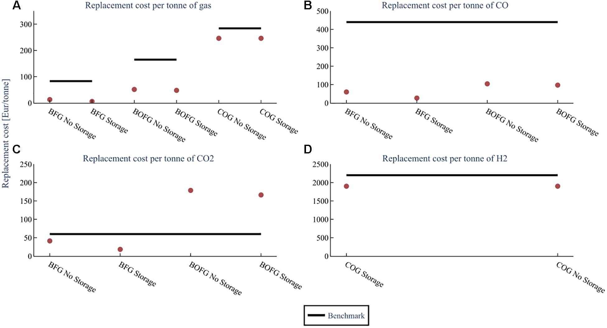
Figure 13. Replacement cost comparison of the three steel mill gases with no storage vs 90 kt storage (optimal) for the base scenario (flare rate 2%, capacity 100 kt BFG). The costs for (A) assume both CO and CO₂ are used. The costs for (B–D) are assuming that feedstock is the only one used. The benchmark is the cost of the feedstock when produced from conventional sources.

FIGURE 14

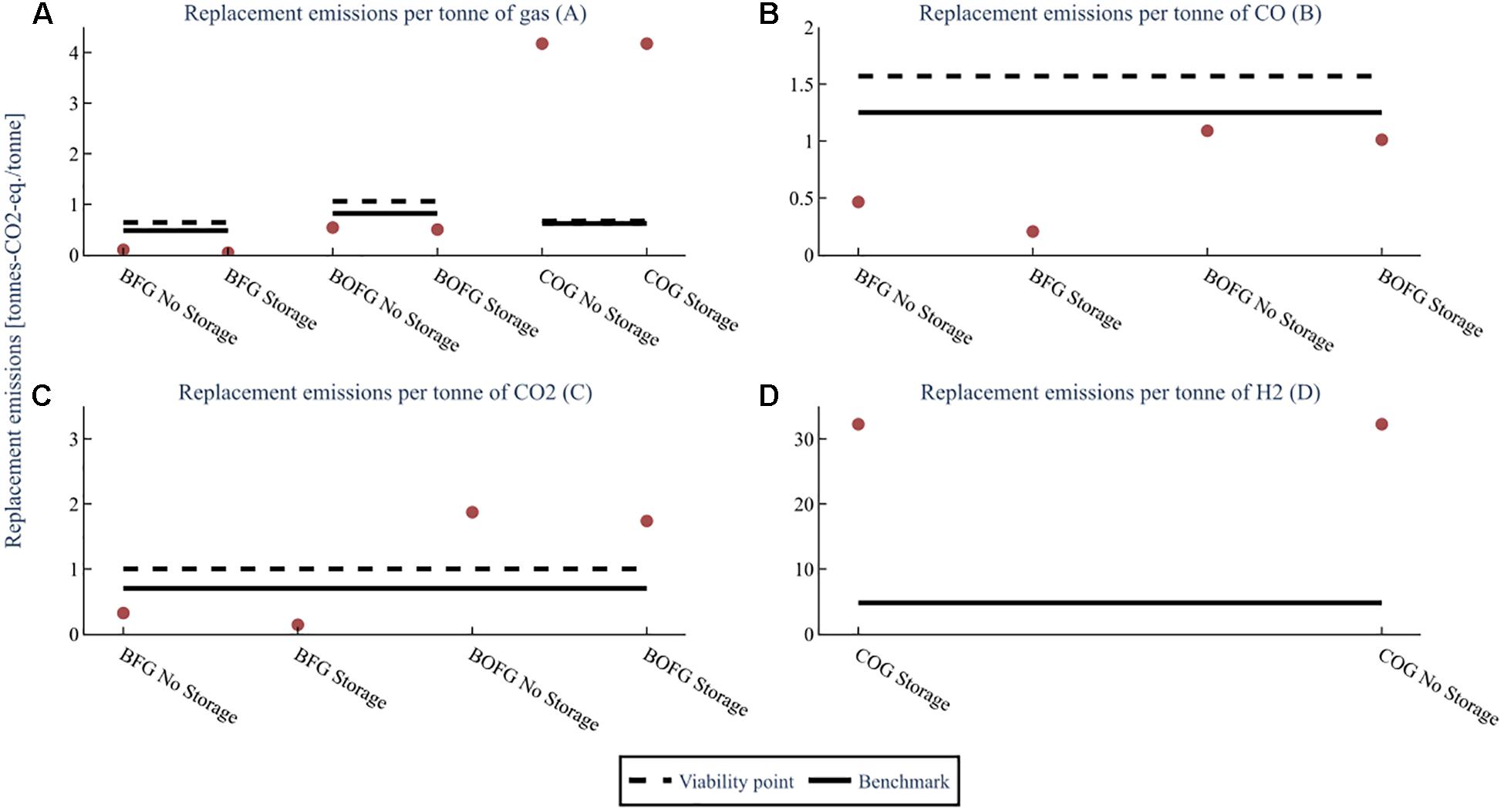
Figure 14. GHG emissions comparison of the three steel mill gases with no storage vs. 90kt storage (optimal) for the base scenario (flare rate 2%, capacity 100 kt BFG). The replacement emissions for (A) assume both CO and CO₂ are used. The replacement emissions for (B–D) are assuming that feedstock is the only one used. The benchmark is the global warming impact of the feedstock when produced from conventional sources.

Discussion

Energy Results

The replacement costs for BFG for both heating and electricity generation are the lowest, followed by BOFG and finally COG, directly correlated to the gases’ calorific value. Heating has a lower replacement cost in Germany than in France, and vice versa for electricity. Electricity taxes and tariffs are significantly higher in Germany than in France, resulting in a more expensive electricity price. However, the price for natural gas in Germany is on average lower than for France. Subsequently, in Germany, only 53.4% of the time grid electricity is used to replace steel mill gases that would otherwise be used in the power plant, compared to 95.4% of the time for France. These values are not expected to vary significantly year on year due to limited changes in the electricity and natural gas price and no significant changes in the average European steel mill. Therefore, the assumption that 2017 data could be used as an effective proxy for steel mill gas replacement costs for other years is reasonable. Naturally, when looking more than 5–10 years into the future, updated electricity and natural gas price data should be used if available.

The different usages of each gas, shown in Figure 7, are less certain to change in other circumstances. The major potential source of uncertainty is the data obtained from the steel producer; although flaring data was obtained from multiple plants and manipulated to try and obtain European average flaring data, it is still inherently based on steel mills from one company, and therefore it is hard to say how accurately they portray flaring patterns for steel mills from other companies. While all steel mills using the conventional route of steel production should be similar, there could be deviations in locations of parts of the plant, making usage of one of the steel mill gases more favorable for heating, for instance. The model used in this study was designed in such a way that enables it to be used for any industrial flue gas stream for which end usage data is available. Therefore, it is recommended to use this model or perform a similar calculation for each steel mill and flue gas utilization scenario desired due to these individual mill differences.

Economic Results

The replacement costs of CO are significantly lower than the benchmark for all scenarios of BFG and BOFG, and the replacement costs for H₂ from COG are slightly lower than the benchmark. Both BFG and BOFG show good economic potential for use as feedstocks for the chemical industry. COG shows good promise as an economically viable H₂ source if it is not required pure; if it is, then the costs of separation would likely put the total cost of H₂ from COG above the benchmark cost. This section discusses and analyses the results based on gas composition, capacity, flare rate, and country.

When used as feedstock for CO, the replacement costs for BFG are about half when compared to the replacement costs for BOFG. When used as feedstock for CO₂, this difference becomes even more pronounced, with BFG’s replacement costs being about four times cheaper per ton of CO₂ obtained. This variance results from the compositional differences of the gases; BOFG has a higher CO composition than BFG and a larger ratio of CO to CO₂ than BFG. BFG has a similar replacement cost per ton of CO or CO₂, whereas obtaining CO from BOFG is about 75% cheaper than obtaining CO₂.

This study finds that larger steel mill gas usage results in a slight increase in replacement cost per unit of feedstock, as shown in Figure 8. As the feedstock requirement increases, there will be fewer times when the flared gas is enough to meet the complete feedstock demand, thus requiring more electricity or heating gas and therefore increasing the value of the gas. For BFG and BOFG, the cost is relatively low and does not vary markedly with respect to capacity. However, this increase in the replacement costs of steel mill gases at increased capacities is low. It should not affect the economic viability of a subsequent chemical production process, especially when taking into account expected decreases in capital costs when building larger plants. COG is comparatively expensive, although it also does not fluctuate too much as capacity changes.

Changes in the flare rate do not have as large an impact on replacement cost as changes in the plant’s capacity (Supplementary Material “Results for Differing Flare Rate Scenarios,” Figure 3). The lack of variation is mainly because steel mill gases are not flared very often, but when they is flared, it is in large amounts, which are more than the required feedstock amount. Although the frequency of flaring increases slightly when the volumetric flare rate increases, this increase is not substantial enough to notice a considerable reduction in gas replacement cost when the flare rate is increased. In general, for both changing flare rates and capacities, the change in the replacement cost of the gas is usually around 10–20% and is not expected to significantly affect a flue gas utilization process’s economic viability. The lack of variation is similar when looking at replacement cost per ton of CO, CO₂, or H₂, where smaller variations are seen with changing flare rate than with changing capacity.

France has lower costs for BFG than Germany and has a broader variation with a similar average cost for BOFG. This wider variation is because BOFG, unlike BFG or COG, is used for electricity generation and heating. Therefore, at lower capacities, BOFG will use mostly electricity gas, which is cheaper in France than in Germany. However, at higher capacities, heating gas must be taken and then natural gas used as a replacement, which is less expensive in Germany. Germany has a lower cost difference between natural gas and electricity, meaning that the cost variation with respect to capacity is smaller.

Costs for the two fossil-fuel-based feedstocks, CO and H₂ from steam reforming, are expected to stay relatively stable as they are established processes. However, with decreasing solar power costs, the production cost of H₂ from electrolysis is expected to drop sharply in the coming decade.

Transportation costs and other capital infrastructure required, such as holding tanks, are not considered in this model. Such costs depend heavily on the distance between the steel mill and the chemical plant, as well as other location-specific logistical factors. Ideally, the chemical plant would be located on or next to the steel mill’s premises, heavily reducing transport costs to almost nothing. In most scenarios, a pipeline would be used to transport the goods. Another source of uncertainty is the profit margin applied by the steel producer, which must be small enough that the cost for the chemical producer is not greater than other feedstocks.

Many previous studies on other chemical processes from steel mill gases do not assume any purchase cost for the gases. This may have a large impact on process economics, particularly for the more valuable COG and BOFG. Even studies that assume zero cost for BFG neglect a cost of multiple million euros per year for mid to large capacity plants. Studies such as Yildirim et al. (2018) that assume COG is to be replaced by natural gas is a more accurate assumption. Taking an average price across 2017 for natural gas in France (31.4 €/MWh) would then result in a replacement cost for COG of 324 €/ton, which is similar to the replacement cost calculated in this study (258 – 280 €/ton), as most COG is used for heating and it has a relatively low flaring rate. It is a slight overestimate due to the share of flare gas that can be used, which does not require a replacement and is not taken into consideration with a static replacement cost assumption. However, if steel mill gas usage data is unavailable, it is a reasonable assumption to make for the replacement cost of COG. Lee et al. (2020) assume that BOFG, as well as COG, will be replaced by natural gas, resulting in a cost for BOFG of 145 €/ton if the study was conducted in France in 2017. This assumption results in a much higher replacement cost than the results presented in this study of 52 – 65 €/ton. This is because only 25% of BOFG is used for heating, while 68% is used for electricity generation; therefore, it would have been more accurate to assume a replacement by grid electricity if a static assumption was desired. As for COG, flaring gas is again neglected, overestimating the replacement cost. The more accurate replacement costs that dynamic cost-minimization models provide could help refine future studies investigating the usage of steel mill gases.

Greenhouse Gas Emissions Results

The GHG emissions required to replace CO from BFG are less than the benchmark and viability point for all three capacity and flaring scenarios, while for BOFG they were only less for the low and mid-capacity scenarios. Therefore, usage of BFG as a feedstock for CO, in particular, is highly recommended from an environmental perspective, reducing the global warming impact of chemical processes. The emissions required to replace H₂ are exceptionally high, about 6 times more than the fossil-fuel-based benchmark. It is not recommended to use COG to obtain H₂ as a feedstock from a global warming impact perspective. In this section, the GHG emissions results will be discussed and analyzed from the standpoint of gas capacity, feedstock, flare rate, and country.

In all scenarios, BFG has low replacement GHG emissions due to its low calorific value; this means less grid electricity or natural gas is required to replace BFG than BOFG or COG. Furthermore, BFG has low replacement GHG emissions due to its comparatively higher share of flare gas, which does not require a replacement. Meanwhile, the replacement emissions when using BOFG as feedstock for CO are about 3–5 times as high as BFG; when using BOFG as a feedstock for CO₂, replacement emissions are 6–10 times as high as BFG. When both are used, the replacement emissions are between 10 and 30 times as high.

As well as for the cost, higher capacities require larger GHG emissions per ton to replace. At low capacities, usage of BOFG for CO can result in a reasonably large emissions savings per ton of CO. Still, the overall capacity is often so low that the total GHG emissions saved are relatively insignificant. As BOFG is the most evenly split between flare gas, electricity gas, and heating gas (see Figure 7), it has the largest range in all scenarios. Smaller capacities use mostly flare gas (which does not require any replacement emissions) and electricity gas, which requires relatively little emissions to replace. Larger capacities use mostly electricity gas and heating gas, which requires moderately high GHG emissions to replace. This is in contrast with BFG, where most of the feedstock comes from either flare gas or electricity gas, resulting in much smaller variations as capacity changes.

As heating gas can only be replaced by natural gas, France has a more extensive range than Germany, due to the considerable average difference in GHG emissions between the electricity grid and natural gas. COG usage results in the same GHG emissions for both Germany and France because no COG is used for electricity generation. Therefore, it is always replaced by natural gas, and the range is due to changes in the amount of flare gas used for different capacities. In the case that COG would also be used for electricity production, perhaps its usage as a feedstock could have a lower global warming potential.

Changes in the flare rate [shown in the Supplementary Material section “Results for Differing Flare Rate Scenarios,” Figure 3)] do not have as large an impact as changes in the plant’s capacity. Again, this is because the frequency of zero flaring does not change drastically, even as the total volumetric flare rate over the year changes significantly.

A source of uncertainty common to industrial symbiosis is which of the two partners should get any credits or certificates for reducing emissions. It may be that due to European regulations, one partner is unable to claim credit for reducing emissions. In all likelihood, any subsidies or avoidance of taxes will likely be passed from one consumer to the other; for instance, the steel mill could claim an emissions reduction and use the money saved to reduce the feedstock costs for the chemical producer.

Previous LCA studies such as Ou et al. (2013) that assume all steel mill gas taken would have otherwise been flared (or give no justification for their assumption of zero replacement emissions) neglect a significant emissions source of 0.26–0.84 tons-CO₂-eq/ton BOFG. COG in particular requires a lot of replacement emissions and would be a large oversight if completely neglected. On the other hand, studies such as Thonemann et al. (2018) that assume natural gas as a replacement for all steel mill gas emissions overestimate the replacement emissions required, particularly for BFG (0.94 tons-CO₂-eq/ton BFG if natural gas was to replace all BFG in France in 2017 compared to 0.02-0.11 tons-CO₂-eq/ton BFG) and BOFG (2.26 tons-CO₂-eq/ton BOFG compared to 0.26–0.84 tons-CO₂-eq/ton BOFG), because most BFG and BOFG are used to generate electricity, and are therefore instead replaced by the electricity grid, which has a lower emissions intensity (particularly in France). As well, the static assumption of natural gas as a replacement does not consider flared gas, which does not need any replacement and therefore lowers the overall replacement emissions. This assumption, however, does not severely overestimate the replacement emissions for COG (5.05 tons-CO₂-eq/ton COG compared to 3.9–4.2 tons-CO₂-eq/ton COG), because COG is mostly used for heating, which is in turn replaced by natural gas. The smaller deviation is due to the amount of flaring gas that can be used, which a dynamic model takes into account. These discrepancies in turn could result in an overestimate for the total emissions estimation for the chemical processes investigated.

It is also important to point out that simply because the replacement emissions required are lower than the emissions that gas would have produced, that does not indicate that every process using this gas as a feedstock will be environmentally favorable. Further processing steps and chemicals needed for a flue gas utilization process will also contain their own emissions footprint, which could make them unviable. The values presented in these plots can simply be used for the replacement emissions required when using steel mill gases as a feedstock in a flue gas utilization process.

2050 Greenhouse Gas Emissions Results

Unlike the economic utility price data, it is expected that the emissions intensity of the electricity grid will change significantly in the future for most countries, particularly for Germany. Although France already has a low emissions-intensity grid, which is not predicted to change greatly until 2050, Germany’s grid has a relatively high emissions intensity, which is expected to decrease drastically by 2050 to levels similar to France. To account for this, the study also analyzed usages for steel mill gases in the 2050 scenarios. If studies into the shorter-term future are desired (such as 2030), the model should be re-run at the expected grid emissions intensities for that year and country. In Figure 10, a strong decrease in the GHG replacement emissions are seen for BFG in Germany between the 2017 (0.43–0.55 tons-CO₂-eq./ton CO) and 2050 (∼0.05–0.06) tons-CO₂-eq./ton CO) scenarios; as most of the BFG is used for electricity generation, changes to the emissions intensity of the grid have a large impact on the replacement emissions required to substitute BFG. The replacement emissions for BOFG in Germany also decrease from 2017 (1.07 – 1.75 tons-CO₂-eq./ton CO) to 2050 (0.47 – 1.47), although not as substantially as for BFG. This is because a smaller fraction of BOFG is used for electricity generation than BFG, so changes to the grid emissions intensity have a smaller effect. Changes in France are not very pronounced for any scenario, due to the small change expected in grid emissions intensity between 2017 and 2050.

Although natural gas was still used in the model for the 2050 scenarios, in reality, it is unlikely to be the most common heating method in 2050. As mentioned in Modeling the Replacement Cost of Steel Mill Gases, a variety of other methods are being investigated that aim to reduce emissions from heating in steel mills. For this reason, the results for the 2050 scenarios are relatively uncertain, with large differences in uncertainty between the three kinds of steel mill gas. The 2050 values for BFG have a higher certainty because very little BFG is used for heating. For BOFG, of which up to 25% used for heating, the uncertainty regarding future heating emissions has a greater effect. COG is even more uncertain, as it is effectively only used for heating. Therefore, the replacement emissions required for BOFG and COG in 2050 could decrease drastically if low-emissions heating technologies are widespread. Likewise, for higher capacity or higher flaring scenarios where more flaring gas is used, the uncertainty decreases, as the fraction of heating gas is lower.

Storage Potential

Use of storage shows substantial reductions in both the replacement costs and emissions for BFG while having a negligible effect for COG and BOFG, because of the larger frequency of flaring for BFG compared to COG and BOFG. As BFG is flared about four times more frequently, the storage tank can be more often replenished with flare gas for BFG than for BOFG and COG. As BFG is not flared in very high frequencies, but large amounts on the occasions when it is flared, utilization of a storage tank allows the possibility to use more flare gas than a scenario without storage.

This result positively highlights the economic and environmental benefits of storage when BFG is used. Although BOFG and COG do not show a substantial decrease in cost or emissions, this could also be different on steel mills that flare these gases more regularly. It is recommended that the idea of storage for BOFG and COG not be discarded, but the model should be run on the data from the particular steel mill that is being considered for a flue gas utilization process.

Data, Scenario, and Model Analysis

As the model directly uses the replacement costs of the steel mill gases to determine the economic value and as an estimate for the cost the chemical producer would pay for the gas, it is robust and versatile and can be used for a range of industrial plants and scenarios beyond what has been investigated in this study. It can be directly used to estimate the economic and environmental feasibility of novel flue gas utilization processes from steel mills, which thus far have not taken into account the economic and environmental cost of utilizing steel mill gases. These processes can be analyzed by using data from published techno-economic or life cycle assessments. Often, this data has to be adapted to fit the novel process. Several parameters are important to note, such as plant capacity, plant location, and the year the study was conducted. As long as the plant’s capacity in the published TEA is also of industrial scale, it is usually possible to directly up-scale the costs according to commonly used factorial methods (Sinnott and Towler, 2009). If much of the process is novel, as is often the case for flue gas utilization processes, it will usually not be possible to conduct a cost estimation based on published literature. In this case, a complete TEA will have to be performed. This TEA can be performed according to standardized guidelines and methods found in literature (Peters et al., 2003; Sinnott and Towler, 2009; Buchner et al., 2018; Zimmermann et al., 2020a,b).

The scenarios chosen for the study were selected to best represent the realistic range of European steel mills, with high, low, and mid flaring rates and gas capacities. Germany and France were selected as they have a large chemical and steel industry, while also having a considerable difference in the electricity grid emissions intensity. Performing the study in different countries could also have a great impact on results, due to the changing grid emissions and utility prices; however, it is likely that Germany and France continue to have substantial chemical and steel industries in the future. The greatest source of uncertainty in the key parameters chosen for the model is the predicted grid emissions intensity for the 2050 scenario; many developments or changes in policy and technology are possible until 2050 that could greatly affect the future grid emission intensity. Therefore, the future grid emissions intensity is quite uncertain. Another potential source of uncertainty is the flaring rate. It is possible that with technological improvements to the integrated steel mill route that flare rates decrease in the future. Decreases in the flare rate would increase the cost of steel mill gases, as less flare gas could be used as feedstock. As well, differences between the flaring rates of individual steel mills could significantly affect the cost of steel mill gases. While the current certainty of flare rates is relatively high, future values are very uncertain. More certain are the gas capacities selected for the study; while process improvements could slightly reduce the amount of steel mill gas required as feedstock for a chemical plant, or slightly larger plants could be built in the future with, respectively, larger feedstocks required, many of these processes are limited stoichiometrically and therefore require at minimum a set amount of a particular component. Therefore, it is expected that the capacities chosen remain relevant for future studies.

A limitation is that the model’s scope does not include any gas separation or purification that may be required for a particular process to use the gas. Many chemical processes may require purer CO or CO₂ or need one or more components removed to avoid interference with desired reactions. However, many chemical processes do not require pure components, such as the Carbon4PUR process, which uses BFG directly (Carbon4PUR, 2020a). An interesting future study would be investigating the costs and emissions involved in the separation and purification of the essential components, such as CO or H₂, as perhaps a more accurate comparison to the benchmarks for processes that require pure component feedstocks.

Conclusion

A promising solution to reduce GHG emissions in the steel industry is industrial symbiosis, using steel mill gases as a feedstock for chemical processes. To correctly estimate such processes’ economic and environmental impact, a model was created to evaluate both the costs and global warming impact of replacing the Current Usages of Steel Mill Gases. The valuable feedstocks from steel mill gases such as CO and H₂ are compared to conventionally produced benchmarks to assess their economic and environmental viability.

The results from this model show that the usage of steel mill gases requires a replacement cost for their current usages in addition to a potential need for separation and purification steps, which lie beyond the scope of this paper. Overall, however, they are a viable source for certain desired feedstocks. BFG in particular is viable as a source of CO and CO₂ from both an economic and environmental perspective with replacement costs between 50 and 70 €/ton CO and GHG emissions between 0.43 and 0.55 tons-CO₂-eq./ton CO, which is both cheaper and less impactful than benchmark feedstocks. BOFG is also recommended as a feedstock in most scenarios, but especially in cases where all the BFG is already being consumed. While it generally performs better than benchmark feedstocks, it performs worse than BFG in most metrics and has a much lower total gas flow than BFG. COG offers the potential for a slight reduction in H₂ cost (1800–2100 €/ton) when compared to conventional production but at the expense of much greater emissions (31 tons-CO₂-eq./ton H₂). BFG can be optimally used in most scenarios with the addition of intermittent storage, allowing for a higher ratio of desirable flare gas to be used.

Potentially interesting future studies could include investigating the economic and GHG emissions cost of gas separation and purification of the feedstocks in order to best compare the results to those of conventional benchmarks. As well, exploring a range of further scenarios such as different future grid emissions intensities, other countries, or additional sources of industrial flue gases.

Data Availability Statement

The raw data supporting the conclusions of this article will be made available by the authors, without undue reservation.

Author Contributions

TS envisaged and developed the methodology and initial model used for economic analysis. BS developed the idea and provided data and guidance for the environmental model. JC performed literature research, data preparation, further advanced the economic model and created the environmental model, and was the main author of all text. AZ and RS provided guidance and structure to the manuscript. All authors read, commented, developed structure, and approved the final manuscript.

Funding

This research was carried out within the project Carbon4PUR, which received funding from the European Union’s Horizon 2020 research and innovation program under grant agreement no. 768919. Furthermore, the research was funded by EIT Climate-KIC, a body of the European Union, project number 180409. The European Commission is neither responsible nor liable for the content of this document.

Conflict of Interest

The authors declare that the research was conducted in the absence of any commercial or financial relationships that could be construed as a potential conflict of interest.

Acknowledgments

The authors would like to thank Natalya Tsoy (Universiteit Leiden) for her help in initializing ideas for the greenhouse gas emissions calculations and finding publicly available data sources for the electricity grid production sources of France. The authors would also like to thank Prof. Sherry Towers for her kind advice.

Supplementary Material

The Supplementary Material for this article can be found online at: https://www.frontiersin.org/articles/10.3389/fenrg.2021.642162/full#supplementary-material

Abbreviations

BFG, blast furnace gas; BOFG, basic oxygen furnace gas; COG, coke oven gas; CHP, combined heat and power plant; GHG, greenhouse gas; LCA, life cycle assessment; TEA, techno-economic assessment.

References

Abanades, J. C., Rubin, E. S., Mazzotti, M., and Herzog, H. J. (2017). On the climate change mitigation potential of CO2 conversion to fuels. Energy Environ. Sci. 10, 2491–2499. doi: 10.1039/c7ee02819a

CrossRef Full Text | Google Scholar

Arens, M., Worrell, E., Eichhammer, W., Hasanbeigi, A., and Zhang, Q. (2017). Pathways to a low-carbon iron and steel industry in the medium-term – the case of Germany. J. Clean. Prod. 163, 84–98. doi: 10.1016/j.jclepro.2015.12.097

CrossRef Full Text | Google Scholar

Aresta, M. (2010). Carbon Dioxide as Chemical Feedstock. Weinheim: WILEY-VCH.

Google Scholar

Artz, J., Müller, T. E., Thenert, K., Kleinekorte, J., Meys, R., Sternberg, A., et al. (2018). Sustainable conversion of carbon dioxide: an integrated review of catalysis and life cycle assessment. Chem. Rev. 118, 434–504. doi: 10.1021/acs.chemrev.7b00435

PubMed Abstract | CrossRef Full Text | Google Scholar

Bellevrat, E., and Menanteau, P. (2009). Introducing carbon constraint in the steel sector: ULCOS scenarios and economic modeling. Rev. Met. Paris 106, 318–324. doi: 10.1051/metal/2009059

CrossRef Full Text | Google Scholar

Bhandari, R., Trudewind, C. A., and Zapp, P. (2014). Life cycle assessment of hydrogen production via electrolysis - a review. J. Clean. Prod. 85, 151–163. doi: 10.1016/j.jclepro.2013.07.048

CrossRef Full Text | Google Scholar

Bruhn, T., Naims, H., and Olfe-Kräutlein, B. (2016). Separating the debate on CO2 utilisation from carbon capture and storage. Environ. Sci. Policy 60, 38–43. doi: 10.1016/j.envsci.2016.03.001

CrossRef Full Text | Google Scholar

Buchner, G. A., Zimmermann, A. W., Hohgr, A. E., äve, and Schomäcker, R. (2018). Techno-economic assessment framework for the chemical industry—based on technology readiness levels. Ind. Eng. Chem. Res. 57, 8502–8517. doi: 10.1021/acs.iecr.8b01248

CrossRef Full Text | Google Scholar

Bundesministerium für Umwelt (2020). Schadstoffregister. Available online at: https://www.bmu.de/themen/bildung-beteiligung/umweltinformation/schadstoffregister/ (accessed on 4 Nov 2020)

Google Scholar

Carbon4PUR (2020a). Carbon4PUR. Available online at: https://www.carbon4pur.eu/ (accessed on: 03 December 2020)

Google Scholar

Carbon4PUR (2020b). Expert communication was conducted in 2020.

Google Scholar

Chauvy, R., Meunier, N., Thomas, D., and De Weireld, G. (2019). Selecting emerging CO2 utilization products for short- to mid-term deployment. Appl. Energy 236, 662–680. doi: 10.1016/j.apenergy.2018.11.096

CrossRef Full Text | Google Scholar

Chen, W. H., Lin, M. R., Leu, T. S., and Du, S. W. (2011). An evaluation of hydrogen production from the perspective of using blast furnace gas and coke oven gas as feedstocks. Int. J. Hydrogen Energy 36, 11727–11737. doi: 10.1016/j.ijhydene.2011.06.049

CrossRef Full Text | Google Scholar

Chiuta, S., Engelbrecht, N., Human, G., and Bessarabov, D. G. (2016). Techno-economic assessment of power-to-methane and power-to-syngas business models for sustainable carbon dioxide utilization in coal-to-liquid facilities. J. CO2 Util. 16, 399–411. doi: 10.1016/j.jcou.2016.10.001

CrossRef Full Text | Google Scholar

CORESYM (2017). CarbOn-Monoxide RE-Use Through Industrial Symbiosis Between Steel and Chemical Industries. Available online at: https://www.metabolic.nl/projects/coresym-industrial-symbiosis/ (accessed November 20, 2021).

Google Scholar

Damodara, V. D. (2018). Numerical modelling of soot emission and flare efficiencies. Int. J. Spray Combust. Dyn. 8, 1–3.

Google Scholar

Deng, L., and Adams, T. A. (2020). Comparison of steel manufacturing off-gas utilization methods via life cycle analysis. J. Clean. Prod. 277:123568. doi: 10.1016/j.jclepro.2020.123568

CrossRef Full Text | Google Scholar

Dufour, J., Serrano, D. P., Gálvez, J. L., Moreno, J., and González, A. (2011). Hydrogen production from fossil fuels: life cycle assessment of technologies with low greenhouse gas emissions. Energy Fuels 25, 2194–2202. doi: 10.1021/ef200124d

CrossRef Full Text | Google Scholar

ENTSOE (2020). Actual Generation Per Production Type. Available online at: https://transparency.entsoe.eu/ (Accessed on 04 Nov 2020).

Google Scholar

EUROFER (2019). Pathways to a CO2-Neutral European Steel Industry. Brussels: EUROFER.

Google Scholar

Fischedick, M., Marzinkowski, J., Winzer, P., and Weigel, M. (2014). Techno-economic evaluation of innovative steel production technologies. J. Clean. Prod. 84, 563–580. doi: 10.1016/j.jclepro.2014.05.063

CrossRef Full Text | Google Scholar

Flores-Granobles, M., and Saeys, M. (2020). Minimizing CO 2 emissions with renewable energy: a comparative study of emerging technologies in the steel industry †. Energy Environ. Sci. 13, 1923–1932. doi: 10.1039/d0ee00787k

CrossRef Full Text | Google Scholar

Fraunhofer (2020). Energy Charts. Munich: Fraunhofer.

Google Scholar

Frey, A., Goeke, V., and Voss, C. (2018). Steel gases as ancient and modern challenging resource; historical review, description of the present, and a daring vision. Chem. Ingen. Tech. 90, 1384–1391. doi: 10.1002/cite.201800046

CrossRef Full Text | Google Scholar

Gabrielli, P., Gazzani, M., and Mazzotti, M. (2020). The role of carbon capture and utilization, carbon capture and storage, and biomass to enable a Net-Zero-CO2 emissions chemical industry. Ind. Eng. Chem. Res. 59, 7033–7045. doi: 10.1021/acs.iecr.9b06579

CrossRef Full Text | Google Scholar

Gagniuc, P. A. (2017). Markov Chains: From Theory to Implementation and Experimentation. Hoboken, NJ: John Wiley & Sons, Inc.

Google Scholar

Gielen, D., Taibi, E., and Miranda, R. (2019). Hydrogen: A Renewable Energy Perspective. Abu Dhabi: International Renewable Energy Agency.

Google Scholar

Harvey, S. P., Knoche, K. F., and Richter, H. J. (1995). Reduction of combustion irreversibility in a gas turbine power plant through off-gas recycling. J. Eng. Gas Turb. Power 117, 24–30. doi: 10.1115/1.2812776

CrossRef Full Text | Google Scholar

Hasanbeigi, A., Arens, M., and Price, L. (2014). Alternative emerging ironmaking technologies for energy-efficiency and carbon dioxide emissions reduction: a technical review. Renew. Sustain. Energy Rev. 33, 645–658. doi: 10.1016/j.rser.2014.02.031

CrossRef Full Text | Google Scholar

He, K., and Wang, L. (2017). A review of energy use and energy-efficient technologies for the iron and steel industry. Renew. Sustain. Energy Rev. 70, 1022–1039. doi: 10.1016/j.rser.2016.12.007

CrossRef Full Text | Google Scholar

Hernández, S., Farkhondehfal, M. A., Sastre, F., Makkee, M., Saracco, G., and Russo, N. (2017). Syngas production from electrochemical reduction of CO2: current status and prospective implementation. Green Chem. 19, 2326–2346. doi: 10.1039/c7gc00398f

CrossRef Full Text | Google Scholar

Ho, M. T., Bustamante, A., and Wiley, D. E. (2013). Comparison of CO2 capture economics for iron and steel mills. Int. J. Greenh. Gas Control 19, 145–159. doi: 10.1016/j.ijggc.2013.08.003

CrossRef Full Text | Google Scholar

Hou, S. S., Chen, C. H., Chang, C. Y., Wu, C. W., Ou, J. J., and Lin, T. H. (2011). Firing blast furnace gas without support fuel in steel mill boilers. Energy Convers. Manag. 52, 2758–2767. doi: 10.1016/j.enconman.2011.02.009

CrossRef Full Text | Google Scholar

IEA (2017). Global Energy and CO2 Status Report. Paris: IEA.

Google Scholar

IEA (2019). The Future of Hydrogen. Paris: IEA.

Google Scholar

Jarraud, M., and Steiner, A. (2014). Climate Change 2014: Synthesis Report. Geneva: IPCC.

Google Scholar

Joseck, F., Wang, M., and Wu, Y. (2008). Potential energy and greenhouse gas emission effects of hydrogen production from coke oven gas in U.S. steel mills. Int. J. Hydrogen Energy 33, 1445–1454. doi: 10.1016/j.ijhydene.2007.10.022

CrossRef Full Text | Google Scholar

Kim, Y. K., and Lee, E. B. (2018). Optimization simulation, using steel plant off-gas for power generation: a life-cycle cost analysis approach. Energies 11, 2884. doi: 10.3390/en11112884

CrossRef Full Text | Google Scholar

Lee, J. K., Shin, S., Kwak, G. J., Lee, M. K., Lee, I. B., and Yoon, Y. S. (2020). Techno-economic evaluation of polygeneration system for olefins and power by using steel-mill off-gases. Energy Convers. Manag. 224:113316. doi: 10.1016/j.enconman.2020.113316

CrossRef Full Text | Google Scholar

Leimkühler, H.-J. (2010). Trends in Energy and CO2 Reduction in the Chemical Process Industry. Weinheim: Wiley-VCH Verlag GmbH & Co.

Google Scholar

Lundgren, J., Ekbom, T., Hulteberg, C., Larsson, M., Grip, C.-E., Nilsson, L., et al. (2013). Methanol production from steel-work off-gases and biomass based synthesis gas. Appl. Energy 112, 431–439. doi: 10.1016/j.apenergy.2013.03.010

CrossRef Full Text | Google Scholar

Mazumdar, D., and Evans, J. W. (2009). Modeling of Steelmaking Processes. Boca Raton, FL: CRC Press.

Google Scholar

Mcbratney, A., and Everitt, B. S. (2002). Geoderma 121, 155–156.

Google Scholar

Mendoza Beltran, A., Cox, B., Chris, M., van Vuuren, D. P., Font Vivanco, D., Deetman, S., et al. (2020). When the background matters: using scenarios from integrated assessment models in prospective life cycle assessment. J. Ind. Ecol. 24, 64–79. doi: 10.1111/jiec.12825

CrossRef Full Text | Google Scholar

Milani, D., Khalilpour, R., Zahedi, G., and Abbas, A. (2015). A model-based analysis of CO2 utilization in methanol synthesis plant. J. CO2 Util. 10, 12–22. doi: 10.1016/j.jcou.2015.02.003

CrossRef Full Text | Google Scholar

Ou, X., Zhang, X., Zhang, Q., and Zhang, X. (2013). Life-cycle analysis of energy use and greenhouse gas emissions of gas-to-liquid fuel pathway from steel mill off-gas in China by the LanzaTech process. Front. Energy 7:263–270. doi: 10.1007/s11708-013-0263-9

CrossRef Full Text | Google Scholar

Pei, P., Korom, S. F., Ling, K., and Nasah, J. (2016). Cost comparison of syngas production from natural gas conversion and underground coal gasification. Mitig. Adapt. Strateg. Glob. Change 21, 629–643. doi: 10.1007/s11027-014-9588-x

CrossRef Full Text | Google Scholar

Peters, M. S., Timmerhaus, K. D., and West, R. E. (2003). Plant Design and Economics for Chemical Engineers, 5th Edn. New York, NY: McGraw-Hill Education.

Google Scholar

PwC (2016). Comparison of Electricity and Gas Prices for Large Industrial Consumers. London: PwC.

Google Scholar

Quadrelli, E. A., Centi, G., Duplan, J.-L. L., and Perathoner, S. (2011). Carbon dioxide recycling: emerging large-scale technologies with industrial potential. ChemSusChem 4, 1194–1215. doi: 10.1002/cssc.201100473

PubMed Abstract | CrossRef Full Text | Google Scholar

Rogelj, J., Shindell, D., Jiang, K., Fifita, S., Forster, P., Ginzburg, V., et al. (2018). “Mitigation pathways compatible with 1.5°C in the context of sustainable development,” in Global Warming of 1.5°C. An IPCC Special Report on the Impacts of Global Warming of 1.5°C Above Pre-Industrial Levels and Related Global Greenhouse Gas Emission Pathways, in the Context of Strengthening the Global Response to the Threat of Climate Change, Sustainable Development, and Efforts to Eradicate Poverty, eds V. Masson-Delmotte, P. Zhai, H. O. Pörtner, D. Roberts, J. Skea, and P. R. Shukla (Geneva: IPCC).

Google Scholar

RTE (2020). Le réseau de Transport de l’électricité. Paris: RTE.

Google Scholar

Sadlowski, M., and Van Beek, M. (2020). Ecologic potential for flexible methanol production from steel mill off-gases. Chem. Ingen. Tech. 92, 1416–1424. doi: 10.1002/cite.202000085

CrossRef Full Text | Google Scholar

SAPEA (2018). Novel Carbon Capture and Utilisation Technologies, no. 2. Berlin: SAPEA.

Google Scholar

Saur, G., and Ramsden, T. (2011). Wind Electrolysis: Hydrogen Cost Optimisation. Washington, DC: Genevieve Saur.

Google Scholar

Sinnott, R., and Towler, G. (2009). Chemical Engineering Design. Amsterdam: Elsevier Ltd.

Google Scholar

Statista. (2020). Steel Industry in Europe - Statistics & Facts 2020. Available online at: https://www.statista.com/topics/6045/steel-industry-in-europe/ (accessed on 18 Nov 2020)

Google Scholar

Stehfest, E., Van Vuuren, D., Kram, T., Bouwman, L., Alkemade, R., Bakkenes, M., et al. (2014). Integrated Assessment of Global Environmental Change with IMAGE 3.0. Model Description and Policy Applications. Nairobi: BESnet.

Google Scholar

Stießel, S., Berger, A., Fernández Sanchis, E. M., and Ziegmann, M. (2018). Methodology for the evaluation of CO2-based syntheses by coupling steel industry with chemical industry. Chem. Ingen. Tech. 90, 1392–1408. doi: 10.1002/cite.201800030

CrossRef Full Text | Google Scholar

Thonemann, N., Maga, D., and Petermann, C. (2018). Handling of multi-functionality in life cycle assessments for steel mill gas based chemical production. Chem. Ingen. Tech. 90, 1576–1586. doi: 10.1002/cite.201800025

CrossRef Full Text | Google Scholar

Towers, S. (2016). Stochastic Compartmental Modelling With Markov Chain Monte Carlo: Part I. Available online at: http://sherrytowers.com/2016/01/02/stochastic-compartmental-modelling-with-markov-chain-monte-carlo/ (accessed July 17, 2020).

Google Scholar

U.S. Department of Energy [DOE] (2010). Final Environmental Assessment for the Blast Furnace Gas Flare Capture Project at the ArcelorMittal USA, Inc. East Chicago: Indiana Harbor Steel Mill.

Google Scholar

Umweltbundesamt (2020). Für Mensch und Umwelt. Available online at: https://www.umweltbundesamt.de/en (Accessed on 04 Nov 2020)

Google Scholar

Uribe-Soto, W., Portha, J. F., Commenge, J. M., and Falk, L. (2017). A review of thermochemical processes and technologies to use steelworks off-gases. Renew. Sustain. Energy Rev. 74, 809–823. doi: 10.1016/j.rser.2017.03.008

CrossRef Full Text | Google Scholar

Wei, W., Mellin, P., Yang, W., Wang, C., Hultgren, A., and Salman, H. (2013). Utilization of Biomass for Blast Furnace in Sweden. Stockholm: KTH Royal Institute of Technology.

Google Scholar

Wernet, G., Bauer, C., Steubing, B., Reinhard, J., Moreno-Ruiz, E., et al. (2016). The ecoinvent database version 3 (part I): overview and methodology. Int. J. Life Cycle Assess. 21, 1218–1230. doi: 10.1007/s11367-016-1087-8

CrossRef Full Text | Google Scholar

Wiley, D. E., Ho, M. T., and Bustamante, A. (2011). Assessment of opportunities for CO2 capture at iron and steel mills: an Australian perspective. Energy Proc. 4, 2654–2661. doi: 10.1016/j.egypro.2011.02.165

CrossRef Full Text | Google Scholar

World Steel Association (2020). World Steel in Figures. Brussels: World Steel Association.

Google Scholar

Worrell, E., Blinde, P., Neelis, M., Blomen, E., and Masanet, E. (2010). Energy Efficiency Improvement and Cost Saving Opportunities in the Fruit and Vegetable Processing Industry - An ENERGY STAR Guide for Energy and Plant Managers. Berkeley, CA: Lawrence Berkeley National Laboratory.

Google Scholar

Wunderlich, J., Armstrong, K., Buchner, G. A., Styring, P., and Schomäcker, R. (2020). Integration of techno-economic and life cycle assessment: defining and applying integration types for chemical technology development. J. Clean. Prod. 287:125021. doi: 10.1016/j.jclepro.2020.125021

CrossRef Full Text | Google Scholar

Yildirim, Ö, Nölker, K., Büker, K., and Kleinschmidt, R. (2018). Chemical conversion of steel mill gases to urea: an analysis of plant capacity. Chem. Ingen. Tech. 90, 1529–1535. doi: 10.1002/cite.201800019

CrossRef Full Text | Google Scholar

Zimmermann, A., and Kant, M. (2017). CO2 Utilisation Today. Available online at: https://www.depositonce.tu-berlin.de/handle/11303/6247 (accessed October 10, 2020).

Google Scholar

Zimmermann, A. W., Jan Müller, L., Marxen, A., Armstrong, K., Buchner, G. A., Wunderlich, J., et al. (2020a). Techno-Economic Assessment & Life Cycle Assessment Guidelines for CO2 Utilization (Version 1.1), 2nd Edn. Ann Arbor, MI: University of Michigan Library.

Google Scholar

Zimmermann, A. W., and Schomäcker, R. (2017). Assessing early-stage CO2 utilization technologies—comparing apples and oranges? Energy Technol. 5, 850–860. doi: 10.1002/ente.201600805

CrossRef Full Text | Google Scholar

Zimmermann, A. W., Wunderlich, J., Müller, L., Buchner, G. A., Marxen, A., Michailos, S., et al. (2020b). Techno-economic assessment guidelines for CO2 utilization. Front. Energy Res. 8:5. doi: 10.3389/fenrg.2020.00005

CrossRef Full Text | Google Scholar