Prediction of the Minimum Film Boiling Temperature of Quenching Vertical Rods in Water Using Random Forest Machine Learning Algorithm

A great amount of research is focused, nowadays, on experimental, theoretical, and numerical analysis of transient pool boiling. Knowing the minimum film boiling temperature (T_min) for rods with different substrate materials that are quenched in distilled water pools at various system pressures is known to be a complex and highly non-linear process. This work aims to develop a new correlation to predict the T_min in the above process: Random forest machine learning technique is applied to predict the T_min. The approach trains a machine learning algorithm using a set of experimental data collected from the literature. Several parameters such as liquid subcooling temperature (T_sub), fluid to the substrate material thermophysical properties (β_f/β_w), and system saturated pressure (P_sat) are collected and used as inputs, whereas T_min is measured and used as the output. Computational results show that the algorithm achieves superior results compared to other correlations reported in the literature.

Introduction

Intensive efforts to understand phase-change processes have increased over the last decade in many industrial sectors. Fusion, solidification, boiling, condensation, and sublimation are several forms of phase-change processes. These processes are widely encountered in energy applications due to their association with latent heat rather than sensible heat. Therefore, they are used in fields such as desalination, metallurgy, electronics cooling, and during thermal generation of electricity and food processing (Collier, 1972).

Recently, a great amount of research has been focused on experimental, theoretical, and numerical analysis of transient pool boiling which is an example of phase-change processes. It is highly favored in various traditional and modern technologies due to its relative simplicity, high heat transfer rate, and low cost. Pool boiling heat transfer occurs when a sufficiently heated surface is submerged in a stagnant pool of a liquid coolant. Initially, the heated surface experiences a film boiling regime where a vapor layer is formed around the heated surface and prevents it from being in direct contact with the liquid coolant (Bonsignore, 1981). Due to the low thermal conductivity of the vapor compared to the liquid, the surface experiences a dramatic decrease in the cooling performance (Hsu, 1972; Jiang and Luxat, 2008). As the temperature of the heated surface decreases, the thickness of the vapor blanket reduces until it collapses at a temperature called Leidenfrost temperature or minimum film boiling temperature (T_min) (Leidenfrost, 1756). At this point, the liquid is able to dramatically cool the heated surface, and the boiling regime transfers from the film to transition boiling. Following that nucleate boiling, natural convection occurs. Since T_min is the boundary between the film and transition boiling, any improvement in its value significantly enhances the heat transfer rate. Thus, investigating the T_min point is essential in areas such as metal heat treating, nuclear engineering industry, in a hypothetical large break loss-of-coolant accident (LOCA), evaporators and compressors in the air conditioning systems, refrigeration systems, chemical processes, and oil systems (Pettersson et al., 2009; Ramesh and Prabhu, 2015). T_min has been widely studied in terms of various parameters such as substrate material (Peterson and Bajorek, 2002), surface conditions and oxidation (Sinha, 2003; Lee et al., 2014), system pressure (Henry, 1974; Sakurai et al., 1984), flow condition (Groeneveld and Stewart, 1982; Carbajo, 1985), initial surface temperature (Kang et al., 2018), rod diameter (Sakurai et al., 1987; Jun-young et al., 2018), liquid subcooling (Adler, 1979; Freud et al., 2009), vapor–liquid contact angle (Ebrahim et al., 2018), surface roughness and microstructure (Peterson and Bajorek, 2002; Carey, 2020), and alternative quenching fluids (Shoji et al., 1990; Lee and Kim, 2017).

In the literature, it was recognized that the complexity and high non-linearity of the film boiling cause difficulty in recognizing the cause–effect relationship, and the prediction of T_min is carried out mostly using correlations developed empirically with many experimental works for certain specific conditions. Recently, Yagov et al. (2021) showed evidence of the existence of the two distinct modes of film boiling during quenching. Steady film boiling of a saturated liquid is one of the most studied boiling regimes, due to the macroscopically impermeable liquid–vapor interface (Aziz et al., 1986; Zvirin et al., 1990). On the other hand, the unsteady film boiling, quenching, of saturated/subcooled water is quantitatively and qualitatively different from the steady one. This study focused on the unsteady film boiling heat transfer for various degrees of liquid subcooling pools, system pressures, and substrate materials. Limited correlations are available in the literature for the estimation of the T_min. Zuber (1958, 1959) utilized Taylor instability analysis to build up a theoretical model to anticipate the minimum heat flux (q_min″). Based on the differences of the gravity-driven density, the continuity of the vapor–liquid interface was demonstrated. The absence of data about the surface properties decreased the accuracy of this correlation since various experimental works noticed that the surface material and the surface roughness significantly affect the T_min (Baumeister et al., 1970; Reed et al., 2013). Berenson (1961) developed a correlation to predict T_min using the Taylor–Helmholtz hydrodynamic instability. He used Zuber’s (1958) correlation for predicting T_min. Since T_min is significantly affected by the wall thermal properties, liquid subcooling, and surface condition, Henry (1974) modified Berenson’s (1961) correlation including different parameters. Baumeister and Simon (1973) explored the impact of different parameters on T_min, for instance, surface conditions, thermal properties of the heated surfaces, the liquid subcooling, and surface conditions. They developed a model to estimate T_min utilizing the combination of an analytical conduction model for isothermal surfaces and experimental data available in the literature for the non-isothermal surfaces (Baumeister et al., 1970), Sakurai et al. (1987) studied tentatively the film boiling heat transfer mechanism on horizontal heated rods quenched in a pool of saturated or subcooled water at different system pressures. The proposed empirical equations were exclusively in terms of the system pressure, which is considered a restriction since T_min is a function of different parameters. Later, Peterson and Bajorek (2002) developed another correlation for T_min which was an extension of Berenson’s (1961) and Henry’s (1974) correlations, taking into account the heat transfer surface properties, liquid subcooling temperature (T_sub), and surface roughness. The mean absolute error (MAE) and the root mean square error (RMSE) were estimated to be 51.38 and 65.47%, respectively. A recent model by Yagov et al. (2018) was developed for copper, nickel, and stainless steel spheres quenched in water at various degrees of liquid subcooling and under atmospheric pressure. The model not only covered a wide range of materials but also the effect of the coolant with an error of ±30%. Ebrahim et al. (2018) developed an empirical correlation that involves the effect of liquid subcooling, surface roughness, and surface substrate material. The correlation was valid between 2 and 15 degrees of liquid subcooling, surface roughness between 0.3 and 0.9 μm, and wall thermal properties from 4.15 × 107 to 8.56 × 107 J-s/m²-K. When accounting for surface roughness, the results showed that the empirical correlation had an MAE of 1.5% and an RMSE of 9.3%. In the absence of the surface roughness value, the correlation predicted T_min with relatively a higher MAE of 10.7% and RSME of 13.3%. Despite that Ebrahim et al. (2018) showed a high dependency for surface roughness on the T_min predictions, surface roughness data are scarce in the literature.

It is worth mentioning that most of the above studies concerning the prediction of T_min have focused on special conditions, which limit their application. In this regard, a more comprehensive forecasting model, with applicability to a wide range of temperature, pressure, and material, needs to be developed.

The present study is focused entirely on predicting the T_min corresponding to the transient film pool boiling. Therefore, the goal of this study is to utilize a robust and reliable kind of machine learning technique called random forest (RF) to predict T_min for various substrate rods quenched in either high- or low-pressure distilled water pools. Utilizing the RF model to predict T_min could be effective in capturing the pattern of large sets of data collected from different experimental investigations.

Modeling

Available Models

Berenson (1961) developed a correlation for the T_min governed by Tylor–Helmholtz hydrodynamic instability mode. The minimum film boiling temperature $T_{min}^B$ is calculated using the following equation:

$$T_{\min }^B=T_{sat}+0.127{\displaystyle \frac{{\mathrm{\rho }}_g{h}_{fg}}{k_g}}{\left[{\displaystyle \frac{g({\mathrm{\rho }}_f-{\mathrm{\rho }}_g)}{{\mathrm{\rho }}_f+{\mathrm{\rho }}_g}}\right]}^{\frac{2}{3}}{\left[{\displaystyle \frac{\mathrm{\sigma }}{g({\mathrm{\rho }}_f-{\mathrm{\rho }}_g)}}\right]}^{\frac{1}{2}}{\left[{\displaystyle \frac{\mathrm{\mu }}{g({\mathrm{\rho }}_f-{\mathrm{\rho }}_g)}}\right]}^{\frac{1}{3}}$$

where T_sat is the saturated temperature, the subscript g refers to the gas/vapor, and f refers to liquid; ρ is a density; k is the thermal conductivity; h_fgis the latent heat of vaporization; μ is the dynamic viscosity; and g is the gravitational acceleration. This correlation agrees with the available experimental measurements within ± 10 percent. Later, Henry (1974) developed a minimum film boiling temperature $T_{\min }^H$ based on the above correlation to include the effects of the wall thermal properties, degree of liquid subcooling, and the surface condition as follow:

$$T_{\min }^H=T_{\min }^B+0.42\left(T_{\min }^B-T_{sub}\right){\left[{\left({\displaystyle \frac{{\mathrm{\beta }}_f}{{\mathrm{\beta }}_{\mathrm{\omega }}}}\right)}^{0.5}{\displaystyle \frac{h_{fg}}{c_{p,\mathrm{\omega }}\left(T_{\min }^B-T_{sat}\right)}}\right]}^{0.6}$$

where T_sub is the subcooled temperature; c_p,ωis the specific heat of the wall; and β_f andβ_w are the thermophysical properties of the fluid and wall, respectively. It is worth mentioning that for both the equations, the vapor properties are evaluated at the film temperature, the liquid properties are evaluated at the liquid bulk temperature, and the wall properties are evaluated at the wall surface temperature.

Data Collection

The model was developed using a total of 379 experimental data points for T_min that have been stated in the literature. All the collected experimental data were collected from research papers that have similar experimental setups as shown in Figure 1 with the exception of Sakurai et al. (1984) data points which were taken from horizontal thin rods. The data were used in a previous work to develop a correlation for T_min using an artificial neural network (Bahman and Ebrahim, 2020). The quenching facility is mainly consisting of a furnace, test sample, pool, and data acquisition (DAQ) system. The furnace is used to heat the test sample to the desired initial temperature before plunging it into the pool. All the test samples have a cylindrical shape, but they vary in length and diameter. Thermocouples are imbedded inside the test samples and are connected to the DAQ system and computer to monitor and measure the test sample temperature during the experiments. A pool with an immersion heater is used to heat the coolant to the desired degrees of liquid subcooling. An immersion thermocouple is placed in the bath to monitor and measure its temperature before, during, and after the quenching process.

FIGURE 1

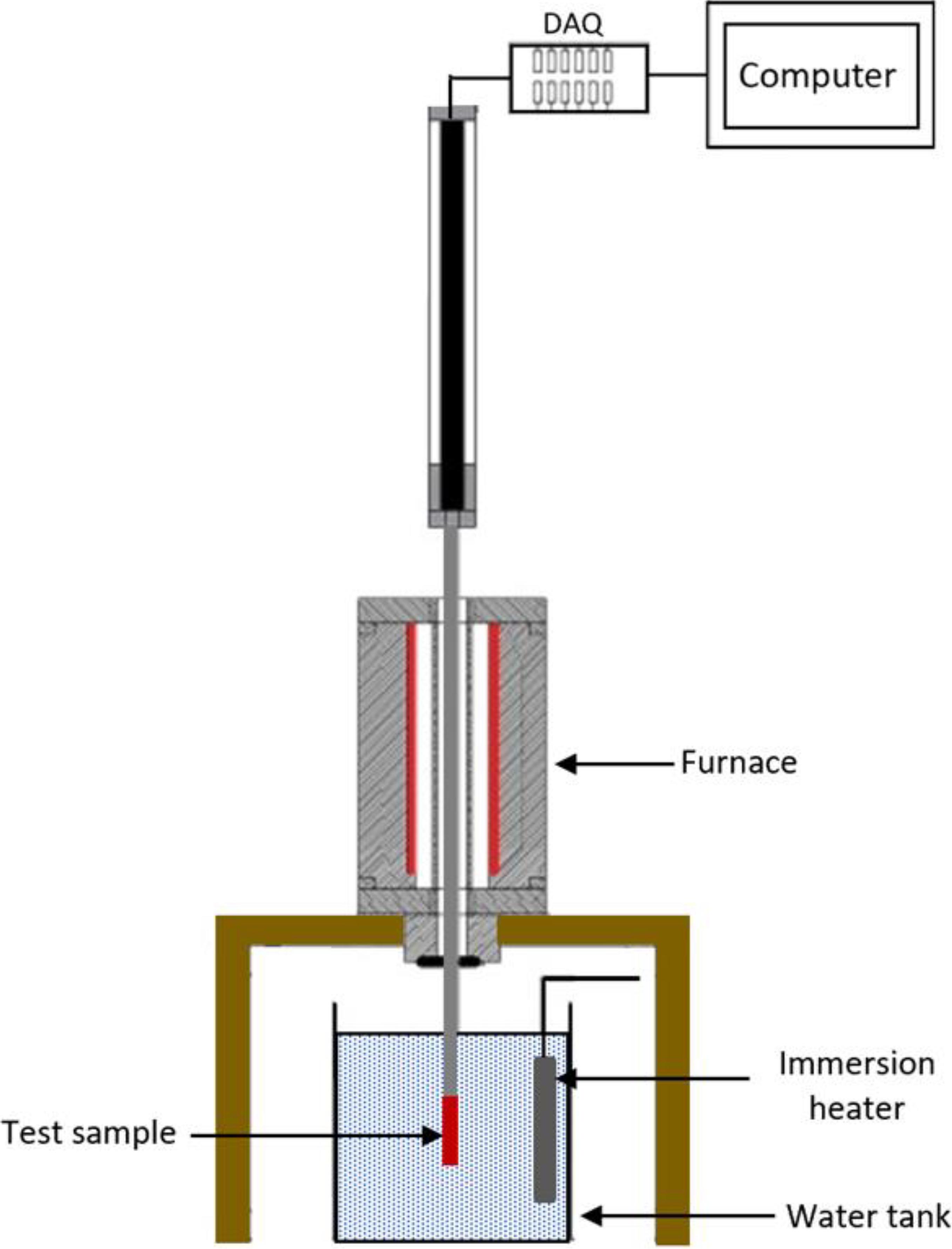
Figure 1. Schematic diagram of the quench facility.

Transient pool boiling heat transfer experiments for various vertical quenched rods in stagnant water baths were conducted to investigate the effect of various parameters on T_min. The quenching conditions vary in the degrees of liquid subcooling, initial rod temperature, saturation pressure, and thermophysical properties as listed in Table 1. The experiments followed similar procedures. First, the rods were heated to a certain initial wall temperature (T_i) in a furnace or a ceramic heater. Then, they were plunged into various degrees of liquid subcooling pools. The temperature of the water in the pool is controlled by an immersion heater and measured by an immersion thermocouple. The degrees of liquid subcooling of the pool represent the difference between the saturation and water temperatures (T_sub = T_sat – T_w). In each rod, thermocouples were embedded at the center and were connected to a DAQ system to monitor and record the temperature before and during the quenching process.

TABLE 1

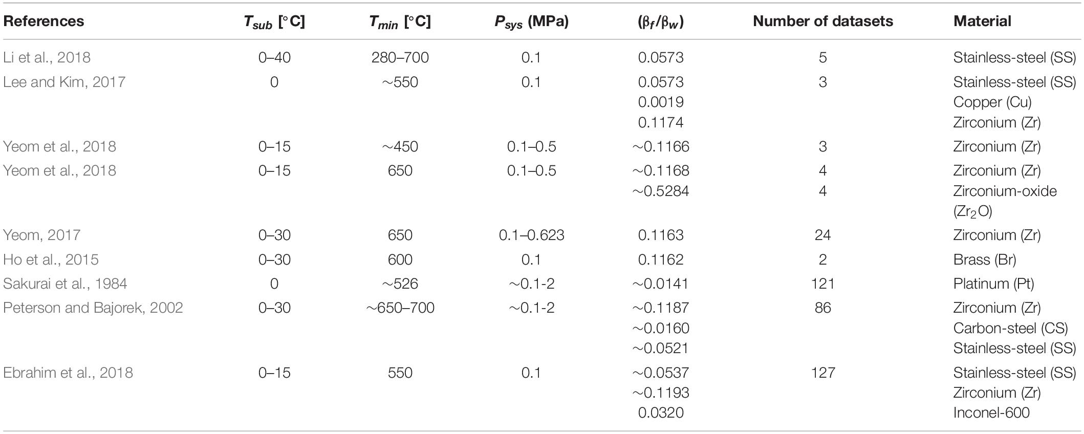
Table 1. Experimental quenching conditions for the collected T_min data from literature.

The input data of the model are taken from different references as shown in the Supplementary Appendix. The summary of datasets is presented in Table 1. The data consist of degrees of subcooling temperature (T_sub), system pressure (P_sys), and substrate material thermophysical properties (β_f/β_w) (thermophysical properties are the product of the density, thermal conductivity, and specific heats β = ρkcp). The Tmin is the output.

Random Forest Algorithm

Machine learning is a group of computer programs aimed toward learning complex problem behavior from data (Ho, 1995; Bishop, 2006). Learning from data has many applications which are categorized as classification, clustering, prediction, and association problems. Most of these algorithms work by presenting a “sample” of problem’s behavioral data to the algorithm in order to create a “human brain” alike computer learning system that is able to understand such problem and generalize, correctly, its response toward never-seen behavioral data for the same problem later. From these algorithms, for example, is the neural network technique, which is being used extensively in thermal system application (Zabirov et al., 2020). The most widely used category of such computer programs is classification algorithm which concerns classifying different data samples into different classes. For example, having correct patient diagnosis data, a classification algorithm can tell, after the learning process, if that patient needs to be hospitalized (aka class 1) or not (aka class 2). Another example from engineering: having preliminary assessments data of the engineering project, one can tell, using a classification algorithm that was trained using assessment data from many previously conducted projects, if that project should be categorized as high risk (aka class 1), risky (aka class 2), low risk (aka class 3), or no risk at all (aka class 4). Many important applications using the classification learning process help different industries.

Decision trees (DTs) are one of the most famous and old classification algorithms as shown in Figure 2. It generates a computational tree that uses, at every branching level, one of the data attributes that mostly minimize the entropy (i.e., degree of randomness) between data classification before branching and after branching. This branching should also increase the information gain within the resulting branches. Each branch has a group of data that can be classified into a possible class or into one of the several classes. A “leaf node” in a DT is that node which is used to make a final discrimination between two different classes of the problem.

FIGURE 2

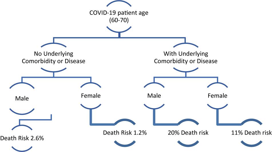
Figure 2. Decision tree example for the classifications of patients with COVID-19 into two classes (Gonçalves and Rouco, 2020).

Random forest is a “Hyper” classification algorithm that combines the decision of an ensemble of DTs into a single decision using some sort of voting model (Ho, 1995). The main idea behind RF is that it samples the training set into N subsets, each of size M, created randomly with replacement from the total set (relative to the number of DTs created), then it uses these subsets to train different DTs separately. This operation, which is called bagging, leads to better model performance because it decreases the variance of the model, without increasing the bias (Breiman, 1994). Once trained, DTs will be used to obtain the predicted class of the remaining data samples, and their different results will be combined in a voting (or averaging) operation to obtain the final classification.

Finally, for the assessment and performance of the model, three criteria, namely, relative error (RE), R-square (R²), and mean square error (MSE) are used. Values of R² closer to 1 mean a higher confidence level of the model, whereas lower values of the RE and MSE are more favorable in terms of model accuracy. These statistical criteria are determined as follows:

$$R{E}_i=\frac{x_{\text{i}}^{\text{experimental}}-x_i^{\text{predicted}}}{x_{\text{i}}^{\text{experimental}}}\times 100$$

$$R^2=1-{\frac{{\sum }_{i=1}^{i=n}\left(x_{\text{i}}^{\text{experimental}}-x_{\text{i}}^{\text{predicted}}\right)}{{\sum }_{i=1}^{i=n}{\left(x_{\text{i}}^{\text{experimental}}-x^{\text{experimental}}\right)}^2}}^2$$

$$MSE=\frac{1}{n}\sum _{i=1}^{i=n}{\left(x_i^{\text{experimental}}-x_i^{\text{predicted}}\right)}^2$$

where $x\overline{{}^{\text{experimental}}}$ is equal to $=\frac{1}{n}{\sum }_{i-1}^n{x}_i$

Methods and Results

Computation experiments were conducted using the RF machine learning algorithm from WEKA Frank et al. (2016) machine learning platform on Intel core i7 with 8GB PC. As mentioned above, the data were collected from different sources used by different researchers to measure T_min. As a start, 379 data samples were used. The data have four main parameters: T_sub, fluid to the substrate material thermophysical properties (β_f/β_w), system saturated pressure (P_sys), material names, and T_min. All were used as inputs except T_min, which was considered as the output. The model was compared with two reported correlations in the literature under specific experimental conditions. Computational experimentations went through multiple phases before the final results were obtained:

(1) Data cleansing phase: Data were analyzed for its suitability for the machine learning process. Some classes (i.e., material types) were immediately removed from the dataset due to the lack of enough samples. Two materials types were found to have very few samples (one has one sample and another has two samples only). Generally, in a machine learning process, you need to have a class of a sample size proportionate to the complexity of the pattern to be learned within the data. Furthermore, you need more samples from each class in the data in order to have some in the training set and some in the testing set as well. Thus, two samples of any class in the problem are considered not enough to learn anything useful. After cleansing those low-represented classes, the total remaining datasets were 373.

(2) Initial analysis phase: The first set of experiments was conducted to see how good the results will be in general without tuning. The experiment used the full data without dividing it into training and testing. As shown in Figure 3A, the model performs well except in some areas where the error margin was relatively high (e.g., samples 133–157). RMSE was 33.19, which is also considered relatively high. This set of experiments revealed the need for further investigation: Looking at the area of high-absolute error and conducting some correlation studies within data samples of the same material types, we found that the data include some “outliers” (few data samples clearly differ from the dominant pattern of the rest of samples and was mostly probably generated via erroneous measurements). Eliminating those data samples resulted in a net total remaining number of 362 clean data.

FIGURE 3

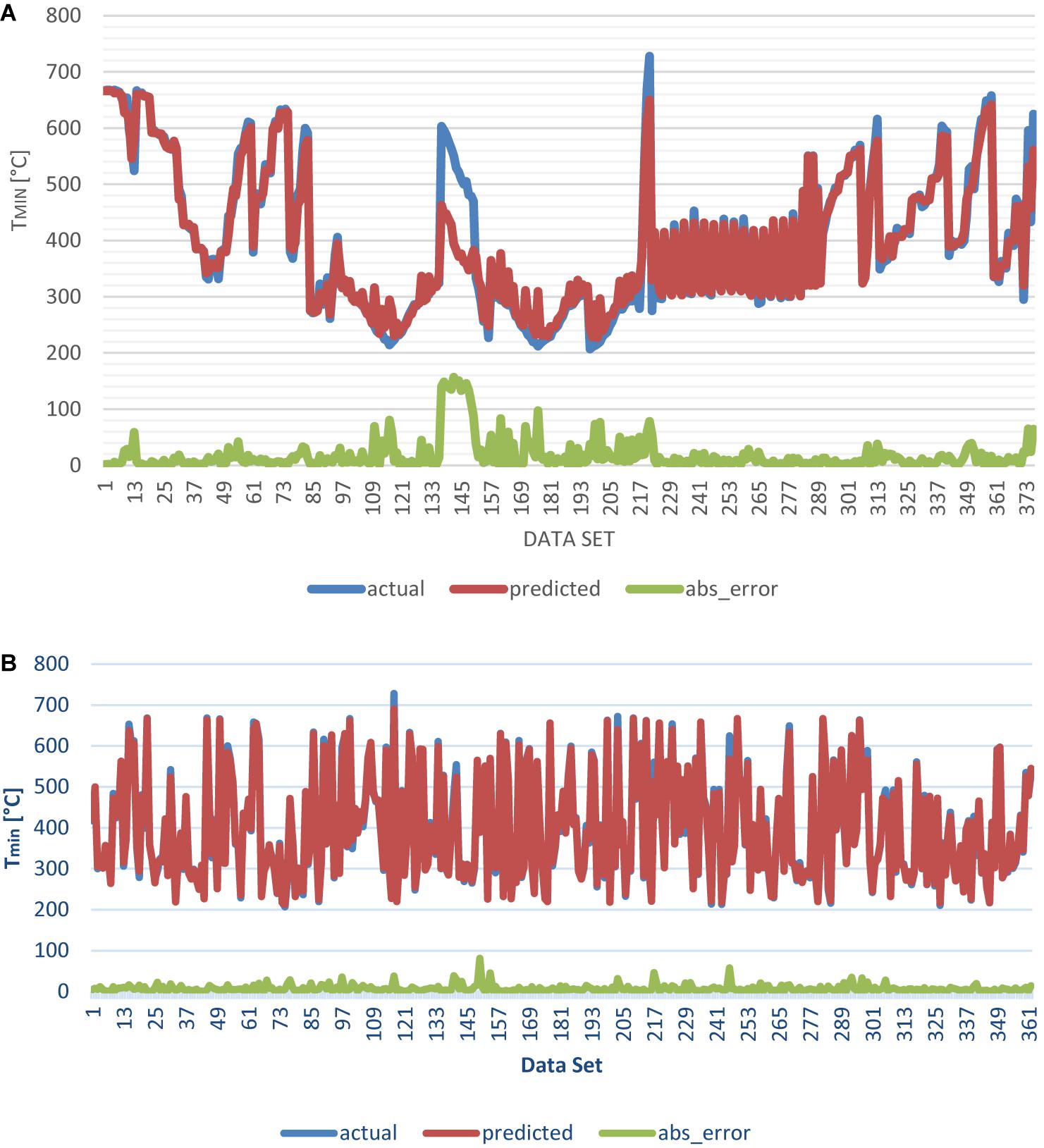
Figure 3. (A) Prediction vs. actual for the full data sample set with absolute error plotted at the bottom of the graph. (B) Prediction vs. actual for the data sample set after removing outliers and applying data reshuffling. Absolute error is shown at the bottom of the graph.

(3) Result analysis phase: In this phase, we run several experiments to analyze the effect of different parameters on the model. In these experiments, the RF model was optimized to give the best results on the training data given. Figure 3B shows the enhancement upon the results when the outliers were removed. RMSE was decreased significantly to 11.3. Parameters and results obtained in model optimizing are shown in Table 2.

TABLE 2

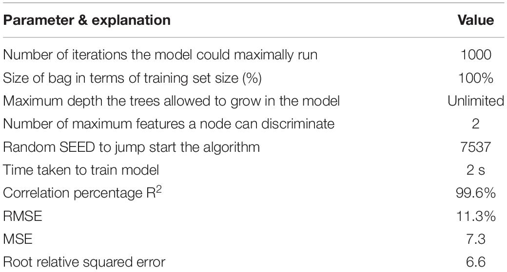
Table 2. Parameters and results for Random Forest prediction model on full data.

(4) Final result phase: The total remaining samples were divided into two parts—308 training sets and 54 testing sets (85% split). We use the same setup of parameters used in the previous phase as shown in Table 2. We ran the algorithm 30 times, and the average number of trees generated was around 200 trees.

In Figure 4, we present the model prediction with the actual 54 experimental datasets. We can see that the RF model performance is excellent in predicting T_min where the R² is 0.9758, which means appropriate prediction of the actual experimental data as shown in Figure 5. In addition to the values of R², the RE of the model for the data was determined. The RE of the model is 4.86%, while in the majority of cases, the RE values were ± 2%. The rest of the results for the RF prediction model on testing the data sample are presented in Table 3.

FIGURE 4

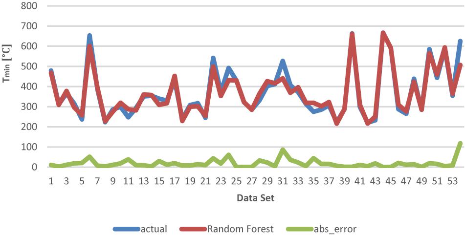
Figure 4. Prediction vs. actual for the testing data sample (54 samples) set with absolute error plotted at the bottom of the graph.

FIGURE 5

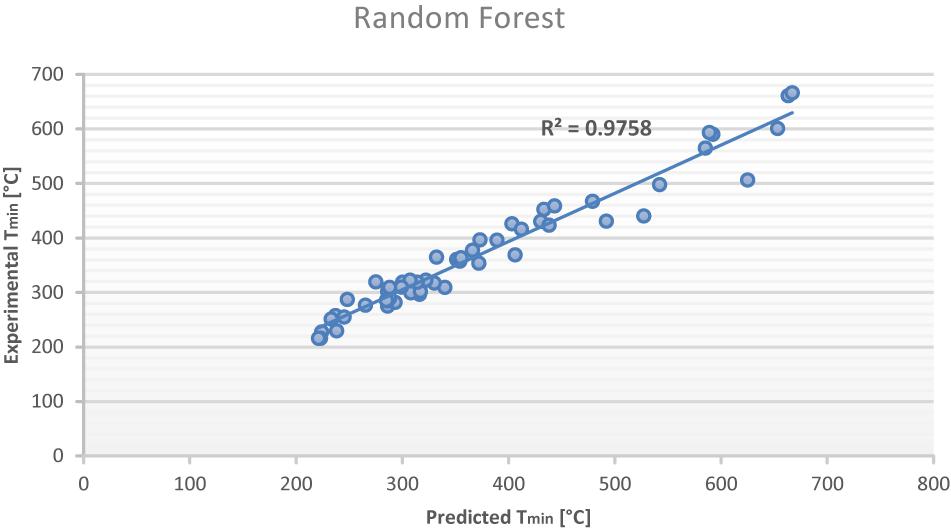
Figure 5. Comparison of RF predicted and experimental minimum film boiling temperature values with testing data.

TABLE 3

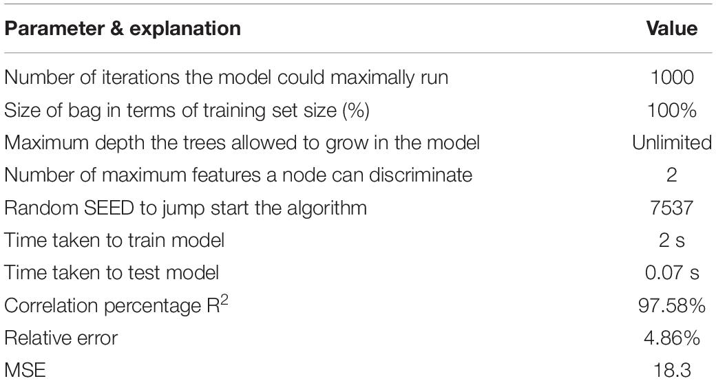
Table 3. Parameters and results for Random Forest prediction model on testing data sample.

Comparing against existing models, the final results of RF were compared with two well-known correlation models obtained in the literature, Berenson (1961) and Henry (1974). The results of the comparison are shown in Figure 6A, where a very good behavior of the RF model in predicting the actual temperature is clear compared to the other models. In Figure 6B, the comparison between the models is presented by a box and whisker model. The median values for the RF model and the actual experimental data are 323 [°C] and 328 [°C], respectively, which were considered very close, whereas for Berenson’s and Henry et al. are 373 [°C] and 402 [°C], respectively, which are far from the actual data. Furthermore, both models failed to capture the lower “whisker” limit compared to RF, while the Henry model relatively captured the upper “whisker” limit better than the RF and Berenson models.

FIGURE 6

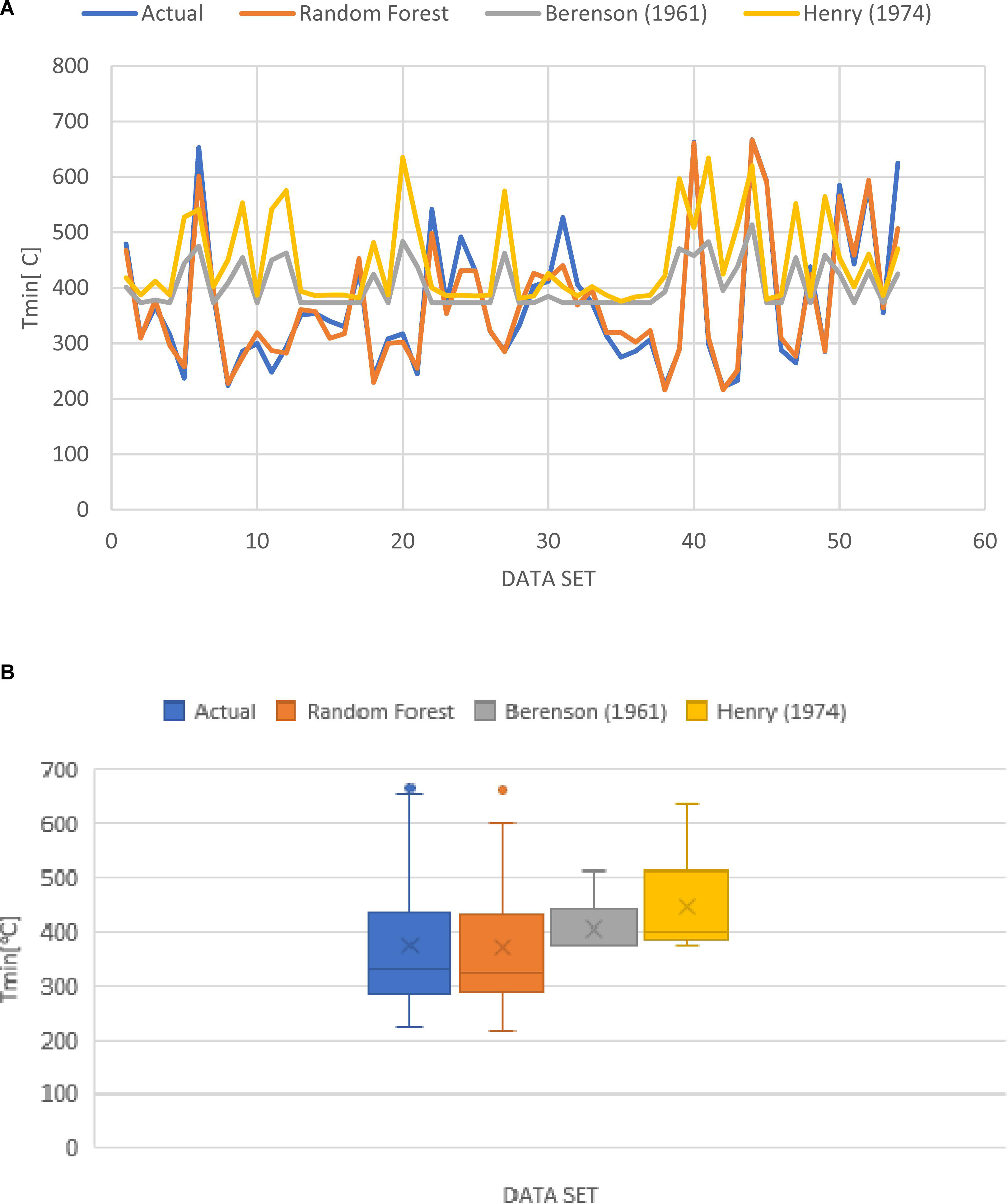
Figure 6. (A) Comparing different models against actual data output. (B) Results obtained by different models compared to actual data output using box and whisker approximation.

The lack of accuracy of Berenson’s (1961) and Henry’s (1974) models compared to the RF in this study was attributed to the developed correlations. Berenson’s correlation was developed by modeling the bubble spacing and growth rate that were determined by using the Taylor instability. The film boiling heat transfer was analyzed by immersing a horizontal surface in n-pentane and carbon tetrachloride at atmospheric pressure. The vapor properties were evaluated at the film temperature and system pressure. Therefore, Berenson’s correlation accounts for the system pressure by changing the vapor properties at different pressures. This correlation does not account for the surface thermophysical properties, surface roughness, and surface wettability, which limit its applications. Henry modified Berenson’s correlation in order to account for the effect of thermophysical properties on T_min, but it does not adequately include the effect of system pressure.

A study by Kang et al. (2018) showed another limitation for Henry’s correlation (1974). They performed experiments on stainless steel (SS) and copper (Cu) rods. The experimental results showed the same value for the T_min, while Henry’s correlation predicted different values due to the difference in the substrate materials. The disagreement between the experimental and predicted data could be due to the other effects such as surface conditions and vapor film collapse mode.

Peterson and Bajorek (2002) concluded that T_min has a strong, positive relationship with pressure at pressures below 1.0 MPa. Therefore, Berenson’s correlation predicts T_min accurately at lower system pressures compared to Henry’s correlation which does not adequately account for a pressure effect on T_min.

Conclusion

A new RF machine learning algorithm was used to formulate a correlation between the T_min for rods with different substrate materials that are quenched in distilled water pools at various system pressures. The resulted model was compared to a well-known correlation model in the literature. Experiments show that the RF model was able by far to predict T_min than the compared ones. One of the drawbacks of the available models is their limited applicability range of input parameters, while the current model is tested in a wide range of all inputs. The key results of the current models can be summarized as follows:

• The RF models were able to confidently forecast the T_min of the quenching rods, with maximum deviations of 13.6%.

• The R² values of the RF-based model were equal to 0.9752.

• The average absolute REs of the RF model are 4.86% and for Berenson and Henry are 33.7% and 43.4%, respectively.

• Among the considered inputs, the T_sub had the greatest impact on the T_min value, followed by the substrate material thermophysical properties (β_f/β_w) and, finally the system pressure (P_sys).

Future works can produce a more generalizable model by utilizing available experimental data for horizontal and vertical flat plates and spheres. In addition, the effect of surface tension and viscosity of the coolant can be involved in the model.

Data Availability Statement

The original contributions presented in the study are included in the article/Supplementary Material, further inquiries can be directed to the corresponding author/s.

Author Contributions

SA devised the work, the main conceptual ideas, and the proof outline. SE provided and verified the data and wrote the background. AS worked out in the computational experimentation. All authors discussed the results and contributed to the final manuscript.

Conflict of Interest

The authors declare that the research was conducted in the absence of any commercial or financial relationships that could be construed as a potential conflict of interest.

Supplementary Material

The Supplementary Material for this article can be found online at: https://www.frontiersin.org/articles/10.3389/fenrg.2021.668227/full#supplementary-material

References

Adler, M. R. (1979). The Influence Of Water Purity and Subcooling on the Minimum Film Boiling Temperature. Ph.D. thesis. Champaign, IL: University of Illinois at Urbana-Champaign.

Google Scholar

Aziz, S., Hewitt, G. F., and Kenning, D. B. R. (1986). “Heat transfer regimes in forced-convection film boiling on spheres,” in Proceedings of the International Heat Transfer Conference Digital Library, (New York, NY: Begel House Inc).

Google Scholar

Bahman, A. M., and Ebrahim, S. A. (2020). Prediction of the minimum film boiling temperature using artificial neural network. Int. J. Heat Mass Transf. 155:119834. doi: 10.1016/j.ijheatmasstransfer.2020.119834

CrossRef Full Text | Google Scholar

Baumeister, K. J., and Simon, F. F. (1973). Leidenfrost temperature—its correlation for liquid metals, cryogens, hydrocarbons, and water. ASME J. Heat Transf. 95, 166–173. doi: 10.1115/1.3450019

CrossRef Full Text | Google Scholar

Baumeister, K. J., Henry, R., and Simon, F. (1970). Role of the Surface in the Measurement of the Leidenfrost Temperature. Technical Report, E-5828. Washington, DC: NASA.

Google Scholar

Berenson, P. J. (1961). Film-boiling heat transfer from a horizontal surface. ASME J. Heat Transf. 83, 351–356. doi: 10.1115/1.3682280

CrossRef Full Text | Google Scholar

Bishop, C. M. (2006). Pattern Recognition and Machine Learning. Berlin: Springer.

Google Scholar

Bonsignore, F. (1981). An Investigation of the Vapor Cushion Thickness, Temperature, and Vaporization Time of Leidenfrost Drops. Master’s Thesis. Rochester (NY): Rochester Institute of Technology.

Google Scholar

Breiman, L. (1994). Bagging Predictors (PDF). Technical Report No. 421. Berkeley: Department of Statistics, University of California.

Google Scholar

Carbajo, J. J. (1985). A study on the rewetting temperature. Nuclear Eng. Des. 84, 21–52. doi: 10.1016/0029-5493(85)90310-3

CrossRef Full Text | Google Scholar

Carey, V. P. (2020). Liquid-Vapor Phase-Change Phenomena: An Introduction to the Thermophysics of Vaporization and Condensation Processes in Heat Transfer Equipment, 3rd Edn. Boca Raton: CRC Press.

Google Scholar

Collier, J. (1972). Convective Boiling and Condensation. New York, NY: McGraw hill.

Google Scholar

Ebrahim, S. A., Chang, S., Cheung, F.-B., and Bajorek, S. M. (2018). Parametric investigation of film boiling heat transfer on the quenching of vertical rods in water pool. Appl. Therm. Eng. 140, 139–146. doi: 10.1016/j.applthermaleng.2018.05.021

CrossRef Full Text | Google Scholar

Frank, E., Hall, M. A., and Witten, I. H. (2016). The WEKA Workbench. Online Appendix for Data Mining: Practical Machine Learning Tools and Techniques, Fourth Edn. Burlington, MA: Morgan Kaufmann.

Google Scholar

Freud, R., Harari, R., and Sher, E. (2009). Collapsing criteria for vapor film around solid spheres as a fundamental stage leading to vapor explosion. Nuclear Eng. Des. 239, 722–727. doi: 10.1016/j.nucengdes.2008.11.021

CrossRef Full Text | Google Scholar

Gonçalves, C. P., and Rouco, J. (2020). Comparing decision tree-based ensemble machine learning models for COVID-19 death probability profiling. J. Vaccines Vaccin. 12:441. doi: 10.1101/2020.12.06.20244756

CrossRef Full Text | Google Scholar

Groeneveld, D. C., and Stewart, J. C. (1982). “The minimum film boiling temperature for water during film boiling collapse,” in Proceedings of the 7th International Heat Transfer Conference, (Germany).

Google Scholar

Henry, R. (1974). A correlation for the minimum film boiling temperature. AIChE Symp. 138, 81–90.

Google Scholar

Ho, T. K. (1995). “Random decision forests (PDF),” in Proceedings of the 3rd International Conference on Document Analysis and Recognition, (Montreal).

Google Scholar

Ho, Y.-H., Ho, M.-X., and Pan, C. (2015). “The effects of subcooling on quenching of a vertical brass cylinder with heating power,” in 2015 Proceedings of the ASME 2015 Nuclear Forum (NUCLRF2015), (Two Park Avenue: American Society of Mechanical Engineers).

Google Scholar

Hsu, Y. Y. (1972). “A review of film boiling at cryogenic temperatures,” in Advances in Cryogenic Engineering. Advances in Cryogenic Engineering, Vol 17, ed. K. D. Timmerhaus (Boston, MA: Springer).

Google Scholar

Jiang, J. T., and Luxat, J. C. (2008). Mechanistic Modeling of Pool Film-Boiling and Quench on a Candu Calandria tube Following a Critical Break LOCA. Switzerland: International Youth Nuclear Congress.

Google Scholar

Jun-young, K., Cheol, L. G., Kaviany, M., Sun, P. H., Moriyama, K., and Hwan, K. M. (2018). Control of minimum film-boiling quench temperature of small spheres with micro-structured surface. Int. J. Multiphase Flow 103, 30–42. doi: 10.1016/j.ijmultiphaseflow.2018.01.022

CrossRef Full Text | Google Scholar

Kang, J.-Y., Kim, T. K., Lee, G. C., Park, H. S., and Kim, M. H. (2018). Minimum heat flux and minimum film-boiling temperature on a completely wettable surface: Effect of the bond number. Int. J. Heat Mass Transf. 120, 399–410. doi: 10.1016/j.ijheatmasstransfer.2017.12.043

CrossRef Full Text | Google Scholar

Lee, C. Y., and Kim, S. (2017). Parametric investigation on transient boiling heat transfer of metal rod cooled rapidly in water pool. Nuclear Eng. Des. 313, 118–128. doi: 10.1016/j.nucengdes.2016.12.005

CrossRef Full Text | Google Scholar

Lee, C. Y., Chun, T.-H., and Kee, W. (2014). Effect of change in surface condition induced by oxidation on transient pool boiling heat transfer of vertical stainless steel and copper rodlets. Int. J. Heat Mass Transf. 79, 397–407. doi: 10.1016/j.ijheatmasstransfer.2014.08.030

CrossRef Full Text | Google Scholar

Leidenfrost, J. G. (1756). De Aquae Communis Nonnullis Qualitatibus Tractatus. Germany: Duisburgi ad Rhenum.

Google Scholar

Li, J. Q., Mou, L. W., Zhang, Y. H., Yu, J. Q., Fan, L. W., and Yu, Z. T. (2018). Pool boiling heat transfer and quench front velocity during quenching of a rodlet in subcooled water: effects of the degree of subcooling. Exp. Heat Transf. 31, 148–160. doi: 10.1080/08916152.2017.1397819

CrossRef Full Text | Google Scholar

Peterson, L. J., and Bajorek, S. M. (2002). Experimental Investigation of Minimum Film Boiling Temperature for Vertical Cylinders at Elevated Pressures. United States: American Society of Mechanical Engineers - ASME.

Google Scholar

Pettersson, K., Chung, H., Billone, M., Fuketa, T., Nagase, F., Grandjean, C., et al. (2009). Nuclear Fuel Behaviour in Loss-of-coolant Accident (LOCA) Conditions. Paris: Organization for Economic Cooperation and Development.

Google Scholar

Ramesh, G., and Prabhu, K. N. (2015). Comparative study of wetting and cooling performance of polymer–salt hybrid quench medium with conventional quench media. Exp. Heat Transf. 28, 464–492. doi: 10.1080/08916152.2014.913088

CrossRef Full Text | Google Scholar

Reed, R. P., Fickett, F. R., Summers, L. T., and Stieg, M. (2013). Advances in Cryogenic Engineering Materials, Vol 40. Berlin: Springer.

Google Scholar

Sakurai, A., Shiotsu, M., and Hata, K. (1984). Effect of system pressure on film-boiling heat transfer, minimum heat flux, and minimum temperature. Nucl. Sci. Eng. 88, 321–330. doi: 10.13182/NSE84-A18586

CrossRef Full Text | Google Scholar

Sakurai, A., Shiotsu, M., and Hata, K. (1987). Transient boiling caused by vapor film collapse at minimum heat flux in film boiling. Nuclear Eng. Des. 99, 167–175. doi: 10.1016/0029-5493(87)90118-x

CrossRef Full Text | Google Scholar

Shoji, M., Witte, L. C., and Sankaran, S. (1990). The influence of surface conditions and subcooling on film-transition boiling. Exp. Therm. Fluid Sci. 3, 280–290. doi: 10.1016/0894-1777(90)90003-p

CrossRef Full Text | Google Scholar

Sinha, J. (2003). Effects of surface roughness, oxidation level, and liquid subcooling on the minimum film boiling temperature. Exp. Heat Transf. 16, 45–60. doi: 10.1080/08916150303749

CrossRef Full Text | Google Scholar

Yagov, V. V., Minko, K. B., and Zabirov, A. R. (2021). Two distinctly different modes of cooling high-temperature bodies in subcooled liquids. Int. J. Heat Mass Transf. 167:120838. doi: 10.1016/j.ijheatmasstransfer.2020.120838

CrossRef Full Text | Google Scholar

Yagov, V. V., Zabirov, A. R., and Kanin, P. K. (2018). Heat transfer at cooling high-temperature bodies in subcooled liquids. Int. J. Heat Mass Transf. 126, 823–830. doi: 10.1016/j.ijheatmasstransfer.2018.05.018

CrossRef Full Text | Google Scholar

Yeom, H. (2017). High Temperature Corrosion and Heat Transfer Studies of Zirconium Silicide Coatings for Light Water Reactor Cladding Applications. Wisconsin: The University of Wisconsin-Madison.

Google Scholar

Yeom, H., Jo, H., Johnson, G., Sridharan, K., and Corradini, M. (2018). Transient pool boiling heat transfer of oxidized and roughened zircaloy-4 surfaces during water quenching. Int. J. Heat Mass Transf. 120, 435–446. doi: 10.1016/j.ijheatmasstransfer.2017.12.060

CrossRef Full Text | Google Scholar

Zabirov, A. R., Amirnova, A. A., Feofilaktova, Y. M., Shevchenko, R. A., Shevchenko, S. A., Yashnikov, D. A., et al. (2020). Using neural networks in atomic energy thermophysical problems. Therm. Eng. 67, 497–508. doi: 10.1134/s0040601520080108

CrossRef Full Text | Google Scholar

Zuber, N. (1958). On the stability of boiling heat transfer. Trans. Am. Soc. Mech. Eng. 80, 711–720.

Google Scholar

Zuber, N. (1959). Hydrodynamic Aspects of Boiling Heat Transfer. Ph.D. Thesis. California: UCLA.

Google Scholar

Zvirin, Y., Hewitt, G. R., and Kenning, D. B. R. (1990). Boiling on free-falling spheres: drag and heat transfer coefficients. Exp. Heat Transf. 3, 185–214. doi: 10.1080/08916159008946386

CrossRef Full Text | Google Scholar