Large-Scale Heterogeneous Computing for 3D Deterministic Particle Transport on Tianhe-2A Supercomputer

1 Introduction

Particle transport plays an important role in modeling many physical phenomena and engineering problems. Particle transport theory has been applied in (Atanassov et al., 2017) astrophysics (Chandrasekhar, 2013), nuclear physics (Marchuk and Lebedev, 1986), medical radiotherapy (Bentel, 2009), and many other fields. The particle transport equation (Boltzmann equation) is a mathematical physics equation describing the particle transport process, and its solution algorithm has always been the key to research in this field. The existing commonly used solutions are divided into two categories, one is the deterministic methods for solving algebraic equations through discrete space, including spherical harmonic method (Marshak, 1947), discrete ordinates method (Carlson, 1955), etc. The other is the stochastic methods, for instance, the Monte Carlo method (Eckhardt, 1987), which simulates particle space using probability theory (Atanassov et al., 2017). With the development of science and technology, simulations of particle transport is more and more demanding of precision and realtimeness. Therefore, facing the rapidly expanding scale of computation and the need for higher performance, it is necessary for researchers to study scalable parallel algorithms for large-scale particle transport.

Currently, the performance of multi-core processors is limited by frequency, power consumption, heat dissipation, etc. And the process of adding cores in a single CPU has encountered bottlenecks. In order to further improve computing performance under existing conditions, the many-integrated-core processors have begun to be used to build high-performance computing systems, including NVIDIA’s GPU (Wittenbrink et al., 2011) and Intel’s MIC (Duran and Klemm, 2012). The latest Top500 list released in November 2020 (TOP500.ORG, 2020), most of the top ten are multi-core heterogeneous systems, including Summit, Sierra, Piz Daint, ABCI, which are based on NVIDIA-GPU and Trinity which uses Intel Xeon Phi processors. The Tianhe-2A supercomputer replaces the Intel Xeon Phi 31S1P accelerators with the independently developed Matrix2000 multi-core accelerators. The whole system has a total of 17,792 heterogeneous nodes, which reaches a peak performance of 100.68 PFlops, and the measured performance reaches at 61.40 PFlops. Heterogeneous parallel computing based on coprocessor has become a trend in the field of high-performance computing, and some achievements have been made in the fields of particle transport (Panourgias et al., 2015), fluid mechanics (Cao et al., 2013) and molecular dynamics (Pennycook et al., 2013).

Scalable parallel algorithm for particle transport is one of the main application fields in high-performance computing. Since the solution of the particle transport equation is related to spatial coordinates, motion direction, energy, and time, its high-precision solution is very time-consuming (Marchuk and Lebedev, 1986). Over the years, the simulation overhead of particle transport problems has dominated the total cost of multiphysics simulations (Downar et al., 2009). Using the current discrete simulation algorithm, a transport solver that completely discretizes all coordinates will require 10¹⁷–10²¹ degrees of freedom (Baker et al., 2012) for each step, even beyond the reach of the Exascale Computing.

Sweep3D (LANL, 2014) is a program for solving single-group steady-state neutron equations and also the benchmark for large-scale neutron transport calculations in the Accelerated Strategic Computing Initiative (ASCI) program established by the U.S. Department of Energy. Many researchers have ported and optimized Sweep3D to heterogeneous systems. Petrini et al. (2007) and Lubeck et al. (2009) migrated Sweep3D to the Cell stream processor in single MPI process mode and multiple MPI process mode, respectively. Gong et al. (2011) and Gong et al. (2012) designed a large-scale heterogeneous parallel algorithm based on GPU by mining fine-grained thread-level parallelism of particle transport problems, which breaked the limitations of the particle simulation and took full advantage of GPU architecture. Wang et al. (2015) designed Sweep3D with thread-level parallelism and vectorization acceleration, and ported Sweep3D to the MIC many-core coprocessors, then applied the Roofline model to access the absolute performance of the optimizations. Liu et al. (2016) presented a parallel spatial-domain-decomposition algorithm to divide the tasks among the available processors and a new algorithm for scheduling tasks within each processor, then combined these two algorithms to solve two-dimensional particle transport equations on unstructured grids.

Based on Sweep3D, we design and develop the method of large-scale heterogeneous computing for 3D deterministic particle transport on Tianhe-2A supercomputer. Compared with original Sweep3D program, this method develops OpenMP thread-level parallelism and implements heterogeneous computing functions based on the Basic Communication Library (BCL) and the Accelerated Computing Library (ACL), which are highly customized for Tianhe-2A.

2 Background

2.1 Sweep3D

The particle transport equation mainly describes the process of collision with the nucleus when the particle moves in the medium, and with its solution we can obtain the distribution of the particle with respect to space and time. According to the particle conservation relationship, the unsteady integral-differential particle transport equation can be obtained. Eq. 1 gives the particle angular flux density expression of the transport equation. $\psi (\vec{r},\vec{\mathrm{\Omega }},E,t)$ represents the particle angular flux density, which is a function of the moving direction $\vec{\mathrm{\Omega }}$, time t, the energy E and the spatial point $\vec{r}$, and v(E) represents the velocity of the kinetic energy E particle, ${\sigma }_t(\vec{r},E)$ indicating the sum of the cross sections of the particle’s collision with the nucleus at the position $\vec{r}$ and energy E. ${\sigma }_s(\vec{r},\overrightarrow{{\mathrm{\Omega }}^{\prime }}\to \vec{\mathrm{\Omega }},E^{\prime }\to E)$ indicates that the moving particles at position $\vec{\mathrm{r}}$ are scattered from energy E and direction $\overrightarrow{{\mathrm{\Omega }}^{\prime }}$ to energy E and direction $\vec{\mathrm{\Omega }}$. $Q_t(\vec{r},\vec{\mathrm{\Omega }},E,t)$ represents source items, including fission sources and exogenous sources.

$\begin{array}{c}\hfill \frac{1}{v(E)}\frac{\partial }{\partial t}\psi (\vec{r},\vec{\mathrm{\Omega }},E,t)+\vec{\mathrm{\Omega }}\cdot ▿\psi (\vec{r},\vec{\mathrm{\Omega }},E,t)+{\sigma }_t(\vec{r},E)\psi (\vec{r},\vec{\mathrm{\Omega }},E,t)\\ \hfill =Q_t(\vec{r},\vec{\mathrm{\Omega }},E,t)+{\int }_{4\pi }{\sigma }_s(\vec{r},\overrightarrow{{\mathrm{\Omega }}^{\prime }}\to \vec{\mathrm{\Omega }},E^{\prime }\to E)\psi (\vec{r},\overrightarrow{{\mathrm{\Omega }}^{\prime }},E^{\prime },t)d\overrightarrow{{\mathrm{\Omega }}^{\prime }}d{E}^{\prime }.\end{array}(1)$

By discretizing the variables t and E in Eq. 1, we can obtain the time-independent single-group particle transport equation, as shown in Eq. 2.

$\vec{\mathrm{\Omega }}\cdot ▿\psi (\vec{r},\vec{\mathrm{\Omega }})+{\sigma }_t(\vec{r})\psi (\vec{r},\vec{\mathrm{\Omega }})=Q_{ext}(\vec{r},\vec{\mathrm{\Omega }})+{\int }_{4\pi }{\sigma }_s(\vec{r},\overrightarrow{{\mathrm{\Omega }}^{\prime }}\to \vec{\mathrm{\Omega }})\psi (\vec{r},\overrightarrow{{\mathrm{\Omega }}^{\prime }})d\overrightarrow{{\mathrm{\Omega }}^{\prime }}.(2)$

The right-hand side of the equation is the source item, including the scattering source and external source. $Q_{ext}(\vec{r},\vec{\mathrm{\Omega }})$ expresses the external source.

In Sweep3D, the discrete ordinate method S_n is used to discretize the angular-direction Ω into a set of quadrature points and discretize the space into a finite mesh of cells. In the angular direction, we choose several specific discrete angular directions Ω_m (m = 1, 2, …, N), so that the integral concerning the direction of Ω is approximated by numerical summation instead, as shown in Eq. 3, where w_m is the weight of integration in the discrete direction Ω_m.

$\psi (\vec{r})={\int }_{4\pi }\psi (\vec{r},\vec{\mathrm{\Omega }})d\vec{\mathrm{\Omega }}=\sum _{m=1}^M{w}_m\psi (\vec{r},{\vec{\mathrm{\Omega }}}_m).(3)$

Integrating both sides of Eq. 2 over the neighboring angular-directions region, ΔΩ_m, of a given discrete angle Ω_m (μ_m, η_m, ξ_m) where μ_m, η_m, ξ_m represent the components of the unit vector of the particle in the direction Ω_m on the X, Y, Z coordinates with respect to ${\mu }_m^2+{\eta }_m^2+{\xi }_m^2=1$, we get the balanced equation as follows:

${\mu }_m\frac{\partial {\psi }_m}{\delta x}+{\eta }_m\frac{\partial {\psi }_m}{\delta y}+{\xi }_m\frac{\partial {\psi }_m}{\delta z}+{\sigma }_t(\vec{r}){\psi }_m=Q_m(\vec{r}).(4)$

The three-dimensional discrete solution of the space is solved by the finite difference method, and the XYZ geometry is represented by an IJK logically rectangular grid of cells, shown in Figure 3. The finite difference method discretizes the geometric space (x_i, y_j, z_k) = (iΔx, jΔy, kΔz), i = 0, 1, …, I; j = 0, 1, …, J; k = 0, 1, …, K, where $\mathrm{\Delta }x=\frac{x_{max}}{I},\mathrm{\Delta }y=\frac{y_{max}}{J},\mathrm{\Delta }z=\frac{z_{max}}{K}$. Then we can get the difference equation as follows:

$\begin{array}{c}\hfill {\mu }_m\frac{{\psi }_{i+\frac{1}{2},j,k,m}-{\psi }_{i-\frac{1}{2},j,k,m}}{\mathrm{\Delta }x}+{\eta }_m\frac{{\psi }_{i,j+\frac{1}{2},k,m}-{\psi }_{i,j-\frac{1}{2},k,m}}{\mathrm{\Delta }y}+\\ \hfill {\xi }_m\frac{{\psi }_{i,j,k+\frac{1}{2},m}-{\psi }_{i,j,k-\frac{1}{2},m}}{\mathrm{\Delta }z}+{\sigma }_{t,i,j,k}{\psi }_{i,j,k,m}=Q_{i,j,k,m}.\end{array}(5)$

To solve the difference Eq. 5, additional auxiliary relations, such as the rhombic difference relation, need to be added:

$\begin{array}{c}\hfill {\psi }_{i,j,k,m}=\frac{{\psi }_{i+\frac{1}{2},j,k,m}+{\psi }_{i-\frac{1}{2},j,k,m}}{2};\\ \hfill {\psi }_{i,j,k,m}=\frac{{\psi }_{i,j+\frac{1}{2},k,m}+{\psi }_{i,j-\frac{1}{2},k,m}}{2};\\ \hfill {\psi }_{i,j,k,m}=\frac{{\psi }_{i,j,k+\frac{1}{2},m}+{\psi }_{i,j,k-\frac{1}{2},m}}{2}.\end{array}(6)$

Sweep3D uses the Source Iteration (SI) method to solve the discrete Eq. 5. Each iteration includes computing the iterative source, wavefront sweeping, computing flux error, and judging whether the convergence condition is met or not. Wavefront sweeping is the most time-consuming part. In the Cartesian geometries (XYZ coordinates and IJK directions), each octant of angle sweeps has a different sweep direction through the mesh grid, and all angles in a given octant sweep the same way. In SI method, Q_i,j,k,m is known. The sweep of S_n method generically is named wavefront (Lewis and Miller, 1984). A wavefront sweep for a given angle proceeds as follows. Every cell (mesh grid) has 4 equations (Eq. 5 plus Eq. 6) with seven unknowns (6 faces plus one central). Boundary conditions initialize the sweep and allow the system of equations to be completed. For any given cell, three known inflows allow the cell center and three outflows to be solved, and then the three outflows provide inflows to three adjoining cells in particle traveling directions. Therefore, there is recursive dependence in all three grid directions. The recursive dependence causes the sweep to be performed in a diagonal wave across the physical space, and Figure 1A gives a sweep of the wavefront from state (a) to state (d).

FIGURE 1

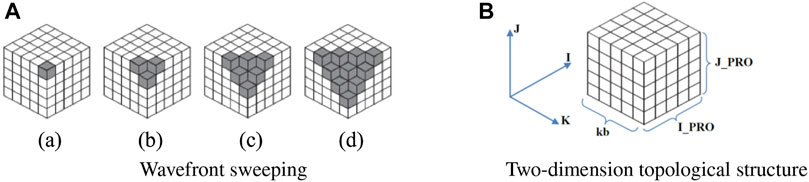
FIGURE 1. Wavefront sweeping and two-dimension topological structure.

Therefore, the parallelism is limited by the length of the JK-diagonal line in Figure 2. To alleviate this problem, MMI angles for each octant are pipelined on JK-diagonal lines to increase the number of parallel I-lines. MMI is the number of angles for blocking and can be chosen as desired, but it must be a integral factor of the number of angles in each octant. Moreover, Sweep3D utilizes Diffusion Synthetic Acceleration (DSA) (Adams and Larsen, 2002) to improve its convergence of source iteration scheme. So wavefront sweeping subroutine mainly involves computing sources from spherical harmonic (P_n) moments, solving S_n equation recursively with or without flux fixup, updating flux from Pn moments, and updating DSA face currents, as shown in Algorithm 1.

FIGURE 2

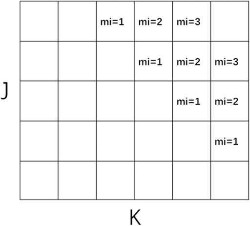
FIGURE 2. This MMI-pipelined JK-diagonal wavefront is depicted below at the fourth stage of a 3-deep wavefront that started in the upper right corner.

Algorithm 1 Wavefront sweeping subroutine in Sweep3D

for iq = 1 to 8 do//octants

 for mo = 1 to mmo do//angle pipelining loop.

  for kk = 1 to kb do//k-plane pipelining loop

   RECV EAST/WEST//recv block I-inflows

   RECV SOUTH/NORTH//recv block J-inflows

   for idiag = 1 to jt + nk − 1 + mmi − 1 do.

    for jkm = 1 to ndiag do//I-lines grid columns

     for i = 1 to it do

      Calculate discrete source term in Pn moments

     if not do fixup then

      for i = 1 to it do

       Solve Sn equation

     else

      for i = 1 to it do

       Solve Sn equation with fixup

     for i = 1 to it do

      Update flux from Pn moments

     for i = 1 to it do

   Update DSA face currents

   SEND East/West//send block I-inflows. SEND North/South//send block J-inflows

2.2 Matrix2000 Accelerator

In the Tianhe-2A supercomputer, each node consists of two Intel Xeon microprocessors and two Matrix2000 accelerators, as shown in Figure 3.

FIGURE 3

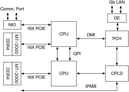
FIGURE 3. Architecture of a computing node.

Each of these Intel Xeon microprocessors is a 12-core processor operating at 2.2 GHz, based on the Intel Ivy Bridge microarchitecture (Ivy Bridge-EX core), with a 22 nm process and a peak performance of 0.2112TFLOPS. The Matrix2000 consists 128 cores, eight DDR4 memory channels, and x16 PCIe lanes. The chip consists of four supernodes (SN) consisting of 32 cores each operating at 1.2 GHz with a peak power dissipation of 240 Watts. Operating at 1.2 GHz, each core has a peak performance of 19.2 GFLOPs (1.2 GHz * 16 FLOP/cycle). With 32 such cores in each SuperNode, the peak performance of each SN is 614.4 GFLOPS. Likewise, with four SN per chip, the peak chip performance is 2.458 TFLOPS double precision or 4.916 TFLOPS single-precision.

3 Scalable Parallel Algorithm for Particle Transport

3.1 Heterogeneous Parallel Algorithms

The process-level parallel algorithm with our method, as shown in Figure 1B, divides the overall mesh space from three directions: I, J, and K. We use a two-dimensional process topology division along the I, J direction for the spatial mesh, so that each K-column mesh along the K direction is stored in a process. Due to the strong data dependency of the sweeping algorithm, in order to improve the parallelism, we need to subdivide the K direction so that each process can quickly complete the data computation of the small mesh and then pass the results to the adjacent meshes in the three directions. The I and J directions are controlled by the process numbers I_PRO and J_PRO, and K direction is controlled by parameter kb. Then we get a mesh space divided into I_PRO*J_PRO*kb mesh of cells.

The sweep calculation is the core of the whole algorithm. Sweeping is running in the diagonal direction of IJK, as shown in Figure 1A. Firstly, in subfigure (a), only the process where the data of the small gray mesh is located performs the calculation, and then passes the results to the three adjacent gray grids along the IJK direction, as shown in subfigure (b), where the two small meshes in the IJ direction are in other processes and the small mesh in the K direction is still in the current process. There is no data dependency between these three small meshes, which can be executed in parallel. Then, the results are transmitted to three adjacent directions, and this operation is repeated to obtain the wavefront sweeping in the order from (a) to (d). Since adjacent mesh involve data dependence, adjacent mesh need to communicate during wavefront sweeping, and lines 4-5 and 20-21 in Algorithm 1 describe this communication process. The idea of our heterogeneous algorithm design is to put all the computations on the Matrix 2000, while the processes on the CPU are only responsible for the MPI communication during the wavefront sweeping.

The heterogeneous communication interfaces supported by the Tianhe-2A supercomputer include OpenMP 4.5, BCL and ACL. Among them, BCL is a simple and efficient symmetric transmission interface, which enables data to be transmitted on the coprocessor and CPU through the PCI-E bus. Although the program migration is more complicated, the transmission rate is faster and the transplant flexibility of the program is better. The heterogeneous program based on the BCL interface needs to compile two sets of programs, which will be running simultaneously on the CPU and the accelerator. First, one of the program is initialized on the CPU, and then the ACL interface is activated to load the other program running on accelerator of the Matrix 2000. The heterogeneous mode flow of our method is given, as shown in Figure 4 and Algorithm 2.

FIGURE 4

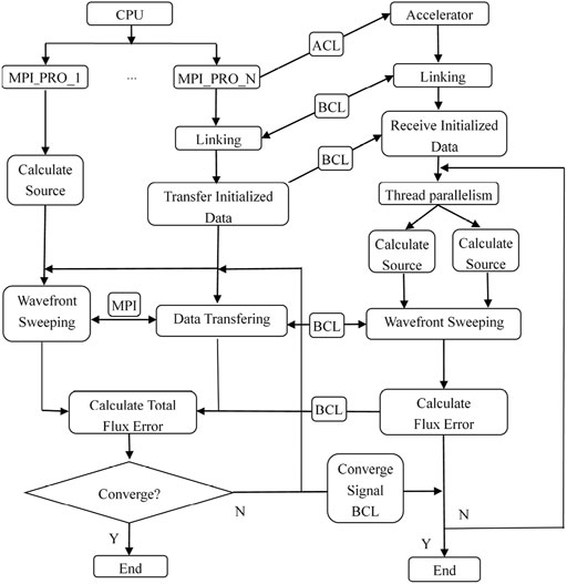
FIGURE 4. Heterogeneous logic flowchart.

First, the CPU starts the MPI to initialize the process, the master process reads the file data, divides the task according to the computing capability, and then transfers the task size to the slave process. Each slave process controls a Matrix2000 supernode and uses the ACL interface to load the programs that need to run on the accelerator of the Matrix 2000, and then establishes a connection between the CPU and the Matrix2000 supernode via the BCL interface. Once the connection is established, the slave processes on the CPU side can communicate with the Matrix2000 via the BCL interface. Then, a small number of parameters are transferred from the slave process to Matrix 2000. The program on the Matrix2000 side receives the parameters and initializes the data directly on the accelerator and proceeds to calculate the iterative source, wavefront sweeping, and compute flux error. Since there is no communication interface between Matrix2000 supernodes, resulting in Matrix2000 supernodes cannot communicate directly and need to go through CPU transition to achieve communication between supernodes. The main function of Matrix2000 supernodes is responsible for intensive data computation. In the wavefront sweeping algorithm 1, the incoming flux and outgoing flux in lines four to five and lines 20-21, respectively, need to involve communication between Matrix2000 supernodes, so the communication between them needs CPU processes to assist.

Algorithm 2 Heterogeneous logic algorithm

if rank_id = 0 then//master process

 Read file and Initialize

 MPI_Send task to slave processes

else

 slave process MPI_Recv the task assigned by the master process//slave process

if rank_id ≠ 0 then//slave process

 Invoke ACL to start the accelerator Matrix2000

 Establish the connection between CPU and Matrix2000

 Invoke BCL to transport initialized data to Matrix2000

 /* the Source Iteration (SI) running on Matrix 2000 */

 #pragma omp parallel for

 {

 Calculate source//Matrix2000

 }

 /* Wavefront sweeping in algorithm 1 */

 for iq = 1 to 8 do

  for mo = 1 to mmo do

   for kk = 1 to kb do

    MPI recv east/west block I-inflows//CPU rank_id

    MPI recv south/north block J-inflows//CPU rank_id

    Invoke BCL to recv the block I-inflows from slave process//Matrix2000

    Invoke BCL to recv the block J-inflows from slave process//Matrix2000

    #pragma omp parallel for

    {

    Calculate discrete source in P_n moments//Matrix2000

    Solve S_n equation//Matrix2000

    Update flux//Matrix2000

    }

    Invoke BCL to send block I-inflows to slave process//Matrix2000

    Invoke BCL to send block J-inflows to slave process//Matrix2000

    MPI send east/west block I-outflows//CPU rank_id

    MPI send south/north block J-outflows//CPU rank_id

 /* Calculate flux error */

 Calculate flux error and invoke BCL to sen//Matrix2000

 

 Calculate total flux error//CPU

 if Converge then

  Invoke BCL to send converge signal to Matrix2000

  Break

 else

  Continuing the calculation in lines 10-30

3.2 OpenMP Thread Level Parallelism

A supernode in Matrix2000 contains 32 cores. In order to fully utilize the performance of Matrix 2000, we use OpenMP instructions to implement thread-level parallelism. Figure 5 shows the optimization process based on OpenMP thread-level parallelism. Among them, the calculation of iterative source, wavefront scanning, and flux error calculation can be performed in thread-level parallel optimization.

FIGURE 5

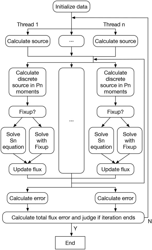
FIGURE 5. OpenMP thread parallelism flowchart.

The iterative source is equal to the sum of the external and scattering iterative sources. As shown in Eq. 7, the scattering iterative source is equal to the product of the flux moment and the discrete cross section, where i represents the ith iteration, and when i = 1, the scattering source can be initialized by any non-negative value.

$Q({\vec{r}}_i)={\sigma }_s(\vec{r})\psi {(\vec{r})}_{i-1}+Q_{ext}(\vec{r})(7)$

When calculating, the grids are independent of each other and have no data dependency. If the single grid is used as the parallel granularity, the overhead of OpenMP scheduling will be too large. Therefore, the IJ plane is used as the parallel granularity, and only the OpenMP thread-level parallelism is performed in the K direction. As shown in Algorithm 3, it is divided into two cases where the discrete order of P_n is 0 and 1.

Algorithm 3 OpenMP thread-level parallelism in source iteration

if isct. Eq. (0) then

 #pragma omp parallel for

 for k = 0; k < kt; k + + do

  for j = 0; j < jt; j + + do.

   for i = 0; i < it; i + + do

    Src(1,k,j,i) = Srcx (k,j) + Sigs (1,k,j,i)*Flux (1,k,j,i) Pflux (k,j,i) = Flux (1,k,j,i) Flux (1,k,j,i) = 0.0

else

 #pragma omp parallel for

 for k = 0; k < kt; k + + do

  for j = 0; j < jt; j + + do

   for i = 0; i < it; i + + do

    Src(1,k,j,i) = Srcx (k,j,i) + Sigs (1,k,j,i)*Flux (1,k,j,i)

    Src(2,k,j,i) = Sigs (2,k,j,i)*Flux (2,k,j,i)

    Src(3,k,j,i) = Sigs (3,k,j,i)*Flux (3,k,j,i)

    Src(4,k,j,i) = Sigs (4,k,j,i)*Flux (4,k,j,i)

    Pflux (k,j,i) = Flux (1,k,j,i)

    Flux (1,k,j,i) = 0.0

    Flux (2,k,j,i) = 0.0

    Flux (3,k,j,i) = 0.0

    Flux (4,k,j,i) = 0.0

Algorithm 4 Iterative OpenMP optimization algorithm in wavefront scanning

#pragma omp parallel for

for jkm = 1 to ndiag do.

 for i = 1 to it do

  Compute source from P_n moments

 if not do fixup then

  for i = 1 to it do

   Solve S_n equation

 else

  for i = 1 to it do

   Solve S_n equation with fixups

 for i = 1 to it do

  Update flux from P_n moments

 for i = 1 to it do

  Update DSA face currents

During the wavefront scanning process, there is a strong data dependency between the wavefronts, and it is not possible to perform calculations in multiple directions at the same time. However, the calculation of all I-line grids in the wavefront of a single direction is independent of each other. OpenMP thread-level parallelism is performed on the I-line grid column, as shown in Algorithm 4. The parallel granularity of threads is limited by the number of I-line grid columns on the JK diagonal. The number of I-line grid columns changes with particles’ movements. The minimum is one and the maximum is the larger of J and K. flushleft.

We determine the flux error by calculating the flux for twice in succession, as shown in Eq. 8, setting the maximum relative error as the overall error value. The calculation of each grid is independent of each other in the process. The JK plane is used as the parallel granularity, and the OpenMP thread-level parallelism is performed from the I direction. The max value in all threads is calculated by the OpenMP reduction statement.

$Erro{r}_{max}=max\left|\frac{\psi ({\vec{r}}_i)-\psi ({\vec{r}}_{i-1})}{\psi ({\vec{r}}_i)}\right|(8)$

3.3 Flux Fixup

Sweep3D solves a single-group, time-independent set of S_n equations on each grid cell. The set of equations consists of the discretized balanced Eq. 9 with three rhombic difference auxiliary Eq. 10, where Eq. 9 is transformed from Eq. 5 combined with the rhombic difference auxiliary equations.

${\psi }_{i,j,k,m}=\frac{1}{D}\left[Q_{i,j,k,m}+A\cdot {\psi }_{i-\frac{1}{2},j,k,m}+B\cdot {\psi }_{i,j-\frac{1}{2},k,m}+C\cdot {\psi }_{i,j,k-\frac{1}{2},m}\right].(9)$

$\begin{array}{c}\hfill {\psi }_{i+\frac{1}{2},j,k,m}=2\cdot {\psi }_{i,j,k,m}-{\psi }_{i-\frac{1}{2},j,k,m}\\ \hfill {\psi }_{i,j+\frac{1}{2},k,m}=2\cdot {\psi }_{i,j,k,m}-{\psi }_{i,j-\frac{1}{2},k,m}\\ \hfill {\psi }_{i,j,k+\frac{1}{2},m}=2\cdot {\psi }_{i,j,k,m}-{\psi }_{i,j,k-\frac{1}{2},m}.\end{array}(10)$

where ${\psi }_{i-\frac{1}{2},j,k,m},{\psi }_{i,j-\frac{1}{2},k,m},{\psi }_{i,j,k-\frac{1}{2},m}$ are the input fluxes of the grid cell (i, j, k) in the I, J and K directions, respectively, ψ_i,j,k,m is the central flux of the cell (i, j, k) for the current dispersion angle, and D, A, B and C represent the relative difference parameters. P_n(spherical harmonic) moments have been used to obtain the source term Q_i,j,k,m. Thus, for a single grid cell in the I-line grid column, the input flux is known, and the central flux of the cell grid can be found, and then the output fluxes ${\psi }_{i+\frac{1}{2},j,k,m},{\psi }_{i,j+\frac{1}{2},k,m}$, and ${\psi }_{i,j,k+\frac{1}{2},m}$ are immediately obtained from the rhombic difference auxiliary Eq. 10. Moreover, in Eq. 9, the central flux ψ_i,j,k,m cannot be negative as long as the input fluxes ${\psi }_{i-\frac{1}{2},j,k,m},{\psi }_{i,j-\frac{1}{2},k,m}$, and ${\psi }_{i,j,k-\frac{1}{2},m}$are not negative, but the output flux obtained by equation Eq. 10 can be negative.

When the negative flux is transmitted along the iterative solution direction, more negative fluxes may be generated, thus triggering fluctuations in the simulation results, and in this case, a negative flux correction is required. In Sweep3D, a zero-setting method is used to correct the negative flux. The iterative solution of the S_n equation with flux correction is similar to that without flux correction, except that the process of negative flux correction is added. The process of flux correction is full of judgments and branches, so it is difficult to exploit the data-level parallelism. Therefore, the iterative solution of the S_n equation with flux correction is still implemented in a serial manner. Lines 5-10 in Algorithm 4 give two different cases of solving the S_n equation with and without flux correction, respectively. For the test cases with different grid sizes and number of threads, the experimental results in Section 4 will give the difference between flux correction or not.

4 Experiment and Results

The benchmark code Sweep3D represents the heart of a real ASCI(Accelerated Strategic Computing Initiative) application established by the U.S. Department of Energy. It solves a 1-group time-independent discrete ordinates (S_n) 3D Cartesian (XYZ) geometry neutron transport problem. Sweep3d is not a program that solves realistic applications, but a realistic S_n code would solve a multi-group problem, which in simple terms is nothing more than a group-ordered iterative solution on top of what Sweep3D does. To keep the problem setup simple, the cross section, external source and geometric array are set to constants in the Sweep3D code. The case of our calculation also follow exactly this simple problem setup.

The test platform is the Tianhe-2A supercomputer. Since ACL and BCL instructions only provide C/C++ interfaces, the implementation of our method is a hybrid encoding of FORTRAN and C. The CPU-side program is compiled with Intel compiler and high-speed network-based MPICH3.2. The accelerator side uses a customized cross-compiler, which supports OpenMP instructions. The compilation option takes ”−O3”. The specifications of test environment and parameters configured for Sweep3D are as shown in Table 1.

TABLE 1

TABLE 1. Specification of the experiment platform.

4.1 OpenMP Performance Optimization Test

In order to effectively evaluate the performance of the OpenMP thread parallel optimization, we run a test with the single-process mode on a CPU core and a Matrix2000 super-accelerated node (32 cores). There are two primary ways to scale Sweep3D on Matrix 2000, including strong scaling and week scaling. Strong scaling means that more cores are applied to the same problem size to get results faster. Weak scaling refers to the concept of increasing the problem size as Sweep3D runs on more cores. This subsection focuses on strong scaling tests, weak scaling tests will be discussed in the next subsection. Table 2 gives the configuration of some parameters of the program during the openMP test.

TABLE 2

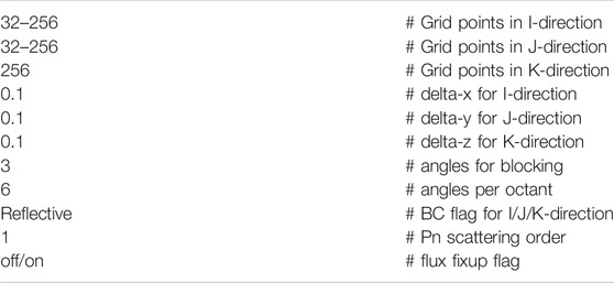
TABLE 2. Parameters configured for sweep3D.

Figure 6 shows the results of four sets of strong scalability tests, where the size of the (I, J, K)-grid is increased from 32 × 32 × 256 to 256 × 256 × 256. To test the performance of the OpenMP algorithm, the four sets of results in Figure 6 give the comparison results for two scenarios with and without flux correction at different (I, J, K)-grid sizes, and each subplot gives the comparison results of time and speedup ratio separately, where the bars indicate the time and the dashes indicate the speedup ratio curves. It can be seen that the computation time of the case without flux correction is less than that of the case with flux correction for all four different problem sizes because performing flux correction increases the number of conditional statements and computation steps in the program code, which leads to an increase in time. From the viewpoint of the speedup ratio, the difference between the speedup ratio curves with and without flux correction is not significant when the grid size is 32 × 32 × 256, especially when the number of threads is 32, the speedup ratio of both cases is approximately equal to 4.7. However, the Figures 6B–D show that as the grid size increases, the difference between the speedup ratio curves of the two cases is small for the number of threads below 8, but the difference becomes larger for 16 and 32 threads. For example, in Figures 6B–D, the network sizes are 64 × 64 × 256, 128 × 128 × 256 and 256 × 256 × 256, respectively, corresponding to a speedup ratio difference of 0.3, 1.2, and 0.9 for 16 threads, and 0.5, 1.6, and 1.8 for 32 threads, respectively.

FIGURE 6

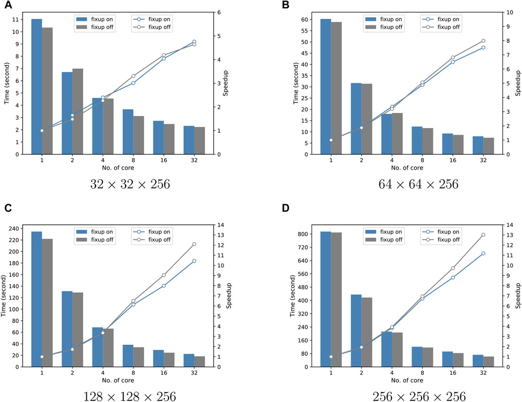
FIGURE 6. Execution time of Sweep3D running on different number of cores in Matrix2000 supernode and speedup in comparison with the simulation on only one core of Matrix 2000. The comparison results for two scenarios with and without flux correction at different (I, J, K)-grid size.

To more intuitively distinguish the difference between with flux fixup and without flux fixup as the grid size increases, Figure 7 exhibits the speedup of Sweep3D running on all 32 cores of Matrix2000 supernode in comparison with that on only one core under different problem sizes. Both with and without flux fixup, the speedup rises gradually with problem size at the beginning, and the speedup between the two flux fixup is still very close at the grid sizes of 32 × 32 × 256, but the difference is gradually increasing as the scale increases, reaching a maximum at 256 × 256 × 256. As the problem size is equal to 256 × 256 × 256, the maximum speedup reach 11.18 and 13.02 for with flux fixup and without flux fixup, respectively. This is because performing flux fixup increases the number of conditional statements and computational steps in the program code, which leads to an increase in time. The time gap between flux fixup and no-fixup becomes smaller as the number of threads increases, but because the single-core time for flux fixup is larger than the no-fixup time, resulting in a smaller speedup ratio, which affects parallel efficiency.

FIGURE 7

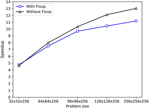
FIGURE 7. Speedup of Sweep3D running on all 32 cores of Matrix 2000 supernode in comparison with that on only one core under different problem sizes.

To better illustrate the results of the strong scaling test for thread-level parallelism, we combine the above data to obtain the results in Figure 8. Figure 8 gives the strong scaling results for a variety of different scales in both with flux fixup and without flux fixup cases. Both subplots show that the performance of the strong scaling test gets better as the size increases, but the efficiency does not reach the desired value as the number of threads reaches 32. There are two main reasons: First, although thread-level parallelism does not involve MPI communication, the computational process in the mesh of a single process is exactly similar to the full-space computational process, which also requires the computational wavefront sweeping process, i.e., the adjacent regions in the mesh also have data dependencies and are also limited by the length of the JK diagonal in the mesh as in Figure 2; Second, the communication between the CPU and Matrix2000 also takes time, which cannot be eliminated by increasing the number of threads.

FIGURE 8

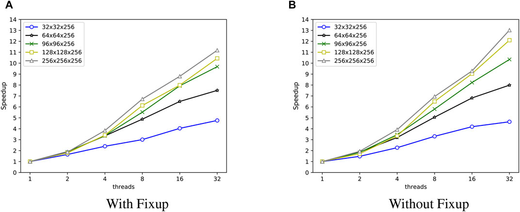
FIGURE 8. Speedup of Sweep3D running on the different problem sizes after by OpenMP optimizing in the two cases of with and without flux fixup.

4.2 Large-Scale Extension Test on Tianhe-2A Supercomputer

We performed a weak scalability test for our method. During the test, we run 8 processes on each node, using 8 CPU cores and 8 Matrix2000 supernodes, and each Matrix2000 supernode starts 32 threads. For the problem sizes, the grid size on a single process remains 32 × 32 × 256, and the size of the K dimension is fixed to 256 while the sizes of the I and J dimensions keep a linear relationship with the number of processes. The test results are given in Table 3.

TABLE 3

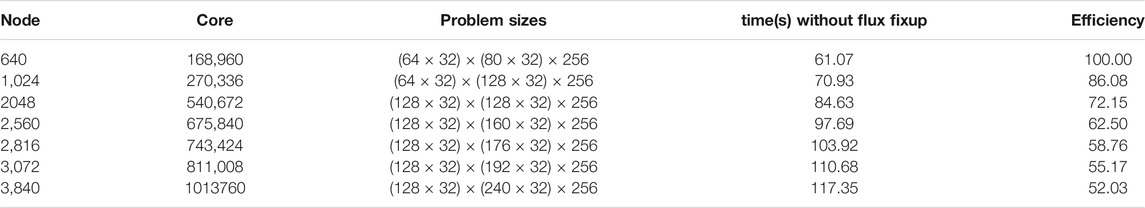
TABLE 3. Weak scaling evaluation.

The correlation between core size and efficiency and time is shown in Figure 9, where the computation time increases slowly and linearly with the number of cores, and the efficiency decreases slowly and linearly with the number of cores. The decisive effect on the parallel efficiency is mainly the strong data dependency between two adjacent wavefronts in the wavefront sweeping algorithm, which requires data communication. As the size increases, that is, the I and J increases, leading to an increase in the number of wavefronts required to complete a global spatial grid sweep, which leads to an increase in communication and causes a decrease in parallel efficiency. Another factor is that the communication between Matrix2000 needs to be relayed through CPUs, which leads to a three-step communication process, adding two CPUs to the Matrix2000 supernode communication process compared to the simple inter-process communication. Although the efficiency decreases as the size increases, our algorithm can still maintain the efficiency of the 540,000 cores versus 170,000 cores is 72%, and the efficiency of the 1.01 million cores versus 170,000 cores is 52% which means much better scalability.

FIGURE 9

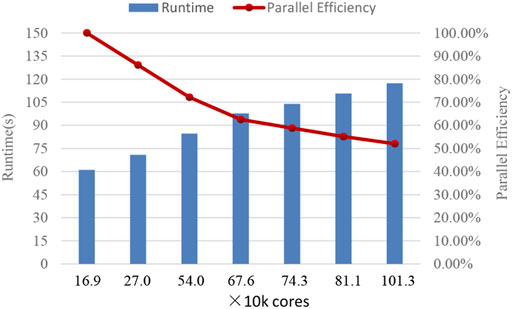
FIGURE 9. Runtime and parallel efficiency on Tianhe-2A.

5 Conclusion and Future Work

We introduce a new method of large-scale heterogeneous computing for 3D deterministic particle transport, which is designed for Tianhe-2A supercomputer. The CPU and Matrix2000 data transmission is completed through the BCL and ACL interfaces. We construct a heterogeneous parallel algorithm to optimize OpenMP on the thread-level parallelism on the Matrix2000 side to improve performance. Our optimization on thread-level parallelism includes iteration source calculation, I-line grid column calculation, and flux error calculation. In the single node test, this method achieves a maximum of 11.3 speedups on the Matrix2000 super-acceleration node. The extension test of the million-core scale was completed on the Tianhe-2A supercomputer, the test efficiency was high, and the program has good scalability. As a part of the future work, we will study on the performance and scalability issues of particle transport algorithms on next-generation China CPU/Accelerator heterogeneous clusters.

Data Availability Statement

The original contributions presented in the study are included in the article/supplementary material, further inquiries can be directed to the corresponding author.

Author Contributions

BL and JL designed heterogeneous parallel algorithm; BL and XZ carried out experiments; BL and SD analyzed experimental results. BL, XZ, and SD wrote the manuscript.

Funding

This work was supported by the National Key Research and Development Program of China (2017YFB0202104, 2018YFB0204301).

Conflict of Interest

The authors declare that the research was conducted in the absence of any commercial or financial relationships that could be construed as a potential conflict of interest.

Publisher’s Note

All claims expressed in this article are solely those of the authors and do not necessarily represent those of their affiliated organizations, or those of the publisher, the editors and the reviewers. Any product that may be evaluated in this article, or claim that may be made by its manufacturer, is not guaranteed or endorsed by the publisher.

Supplementary Material

The Supplementary Material for this article can be found online at: https://www.frontiersin.org/articles/10.3389/fenrg.2021.701437/full#supplementary-material

References

Adams, M. L., and Larsen, E. W. (2002). Fast Iterative Methods for Discrete-Ordinates Particle Transport Calculations. Prog. Nucl. Energ. 40, 3–159. doi:10.1016/s0149-1970(01)00023-3

CrossRef Full Text | Google Scholar

Atanassov, E., Gurov, T., Ivanovska, S., and Karaivanova, A. (2017). Parallel Monte Carlo on Intel Mic Architecture. Proced. Comp. Sci. 108, 1803–1810. doi:10.1016/j.procs.2017.05.149

CrossRef Full Text | Google Scholar

Baker, C., Davidson, G., Evans, T. M., Hamilton, S., Jarrell, J., and Joubert, W. (2012). “High Performance Radiation Transport Simulations: Preparing for Titan,” in SC’12: Proceedings of the International Conference on High Performance Computing, Networking, Storage and Analysis (IEEE), Salt Lake, November 10–16, 2012, 1–10. doi:10.1109/sc.2012.64

CrossRef Full Text | Google Scholar

Bentel, G. C. (2009). Radiation Therapy Planning. New York, NY: McGraw Hill Professional.

Cao, W., Xu, C. F., and Wang, Z. H. (2013). Heterogeneous Computing for a CFD Solver on GPU/CPU Computer. Adv. Mater. Res. 791, 1252–1255. doi:10.4028/www.scientific.net/amr.791-793.1252

CrossRef Full Text | Google Scholar

Carlson, B. G. (1955). “Solution of the Transport Equation by Sn Approximations,”. Technical Report (N. Mex: Los Alamos Scientific Lab). doi:10.2172/4376236

CrossRef Full Text | Google Scholar

Chandrasekhar, S. (2013). Radiative Transfer. New York, NY: Courier Corporation.

Downar, T., Siegel, A., and Unal, C. (2009). Science Based Nuclear Energy Systems Enabled by Advanced Modeling and Simulation at the Extreme Scale. Citeseer.

Duran, A., and Klemm, M. (2012). “The Intel® many Integrated Core Architecture,” in 2012 International Conference on High Performance Computing & Simulation (HPCS) (IEEE), Madrid, Spain, July 2–6, 2012, 365–366. doi:10.1109/HPCSim.2012.6266938

CrossRef Full Text | Google Scholar

Eckhardt, R. (1987). Stan ulam, john von neumann, and the monte carlo method. Los Alamos Sci. 15, 131–136.

Google Scholar

Gong, C., Liu, J., Chi, L., Huang, H., Fang, J., and Gong, Z. (2011). Gpu Accelerated Simulations of 3d Deterministic Particle Transport Using Discrete Ordinates Method. J. Comput. Phys. 230, 6010–6022. doi:10.1016/j.jcp.2011.04.010

CrossRef Full Text | Google Scholar

Gong, C., Liu, J., Huang, H., and Gong, Z. (2012). Particle Transport with Unstructured Grid on Gpu. Comp. Phys. Commun. 183, 588–593. doi:10.1016/j.cpc.2011.12.002

CrossRef Full Text | Google Scholar

LANL (2014). [Dataset]. The Asci Sweep3d Benchmark. Available at: http://wwwc3.lanl.gov/pal/software/sweep3d/.

Google Scholar

Lewis, E., and Miller, W. (1984). Computational Methods of Neutron Transport. New York, NY: John Wiley and Sons, Inc.

Liu, J., Lihua, C., Qing Lin, W., Chunye, G., Jie, J., Xinbiao, G., et al. (2016). Parallel Sn Sweep Scheduling Algorithm on Unstructured Grids for Multigroup Time-dependent Particle Transport Equations. Nucl. Sci. Eng. 184, 527–536. doi:10.13182/NSE15-53

CrossRef Full Text | Google Scholar

Lubeck, O., Lang, M., Srinivasan, R., and Johnson, G. (2009). Implementation and Performance Modeling of Deterministic Particle Transport (Sweep3d) on the Ibm Cell/be. Sci. Program. 17, 199–208. doi:10.1155/2009/784153

CrossRef Full Text | Google Scholar

Marchuk, G., and Lebedev, V. (1986). Numerical Methods in the Theory of Neutron Transport. New York, NY: Harwood Academic Pub.

Marshak, R. (1947). Note on the Spherical Harmonic Method as Applied to the Milne Problem for a Sphere. Phys. Rev. 71, 443. doi:10.1103/PhysRev.71.443

CrossRef Full Text | Google Scholar

Panourgias, I., Weiland, M., Parsons, M., Turland, D., Barrett, D., and Gaudin, W. (2015). “Feasibility Study of Porting a Particle Transport Code to Fpga,” in International Conference on High Performance Computing, Frankfurt, Germany, July 12–16 (Springer), 139–154. doi:10.1007/978-3-319-20119-1_11

CrossRef Full Text | Google Scholar

Pennycook, S. J., Hughes, C. J., Smelyanskiy, M., and Jarvis, S. A. (2013). “Exploring Simd for Molecular Dynamics, Using Intel® Xeon® Processors and Intel® Xeon Phi Coprocessors,” in 2013 IEEE 27th International Symposium on Parallel and Distributed Processing (IEEE), Cambridge, MA, May 20–24, 2013, 1085–1097. doi:10.1109/IPDPS.2013.44

CrossRef Full Text | Google Scholar

Petrini, F., Fossum, G., Fernández, J., Varbanescu, A. L., Kistler, M., and Perrone, M. (2007). “Multicore Surprises: Lessons Learned from Optimizing Sweep3d on the Cell Broadband Engine,” in 2007 IEEE International Parallel and Distributed Processing Symposium (IEEE), Rome, March 26–30, 2007, 1–10. doi:10.1109/IPDPS.2007.370252

CrossRef Full Text | Google Scholar

TOP500.ORG (2020). [Dataset]. Top500 List. Available at: https://www.top500.org/lists/top500/.

Google Scholar

Wang, Q., Liu, J., Xing, Z., and Gong, C. (2015). Scalability of 3d Deterministic Particle Transport on the Intel Mic Architecture. Nucl. Sci. Tech. 26. doi:10.13538/j.1001-8042/nst.26.050502

CrossRef Full Text | Google Scholar

Wittenbrink, C. M., Kilgariff, E., and Prabhu, A. (2011). Fermi Gf100 Gpu Architecture. IEEE Micro 31, 50–59. doi:10.1109/mm.2011.24

CrossRef Full Text | Google Scholar