Deep Learning-Based Prediction of Wind Power for Multi-turbines in a Wind Farm

Introduction

With the emphasis on environmental issues, developing clean energy represented by wind energy and solar energy (Yang et al., 2019a; Yang et al., 2020) is the direction of the energy revolution. In recent years, the solar energy has been rapidly developed (Yang et al., 2019b). The wind power has attracted much attention for its richer resources and efficient power generation technology (Liu et al., 2016). The Global Wind Energy Development Report 2019 shows that the newly installed capacity of global wind turbines in 2019 is 60.4 GW. Due to the randomness and uncertainty of the wind, the large-scale uncontrollable wind power could affect the stability of the power grid, when it is connected to the grid. The dispatch methods of wind farms are required to satisfy the power demand of the grid, which are mainly based on the average distribution method (Yang et al., 2021) and the proportional distribution method (Hazari et al., 2017) at present. However, the topographic effect, wake effect, turbulence intensity and other influencing factors in large wind farms make the wind captured by wind turbines vary at different locations (Song et al., 2021a). In order to avoid the instability of the power grid, for each wind turbine in a wind farm, its power distribution needs to be determined according to its own operating conditions, which requires the power prediction for each wind turbine (Song et al., 2021b).

In the past, there are two types of wind power prediction methods, including the physical method of analyzing the physical quantity to obtain the wind speed data and then converting it into the power data (Seo et al., 2019), and the statistical method for establishing wind power prediction models by collecting the historical data through the Supervisory Control and Data Acquisition system of wind farms and then fitting curves. When most studies focus on predicting the total power of the wind farm or a single wind turbine, few studies aim at the prediction for the power of multiple wind turbines.

Making use of temporal correlation and spatial correlation (i.e., spatiotemporal correlation) in a wind farm could be helpful for multi-location wind power prediction (Jinfu et al., 2019). Since the wind faced by each wind turbine interacts in time and space, the power of a wind turbine is closely related to the wind at its location. In time, there is a certain correlation between the historical state of the wind at the same spatial point, that is, the temporal correlation; in space, winds in different spatial positions at the same time can also affect each other, that is, the spatial correlation. There could be a certain connection between the winds in different times and in different spaces, which is referred to as the spatiotemporal correlation. Nevertheless, it remains a challenge on how to combine the spatiotemporal correlation to solve the power prediction of multiple wind turbines in a wind farm.

In recent years, deep learning methods have been rapidly developed, and been recently used for the wind energy prediction. Compared with traditional machine learning methods, deep learning has better performance in terms of the feature extraction and model generalization. Among typical deep learning methods, Long Short-Term Memory Network (LSTM) shows the excellent performance when dealing with time series problems (Hochreiter and Schmidhuber, 1997), while Convolutional Neural Network (CNN) has an outstanding performance when processing data with spatial structure (Lecun et al., 2015). To take advantage of the spatiotemporal correlation, it is proposed a LSTM-CNN joint model for predicting the wind power of multiple wind turbines in this study. Specifically, LSTM captures the temporal dependence between the wind power data of each single wind turbine, and CNN extracts the spatial correlation between the wind power data of multiple wind turbines. In this way, the joint model learns the interaction between the winds in the wind farm and the wind dynamics with spatiotemporal properties, thus providing the precise prediction information for the wind turbines in the wind farm.

The remainder of this paper is organized as follows. In Section 2, the LSTM-CNN power prediction model is explained. Experimental validation and result analysis are shown in the Section 3. Finally, Section 4 concludes the paper.

The Proposed LSTM-CNN Joint Prediction Model

The difficulty of conducting the temporal-spatial sequence prediction, such as “wind turbine power prediction,” is to simultaneously extract the time dependence and spatial features hidden in the data. After data preprocessing, the LSTM-CNN joint prediction model is proposed, which exploits a two-stage modeling strategy. In the first stage, the temporal features are extracted by the LSTM sub-model. In the second stage, the spatial correlation from the spatial matrix is determined by the CNN sub-model. On this basis, the algorithm training is explained.

Data Preprocessing

Giving that the neural network is very sensitive to the diversity of the input data, and that the uncertainty of the wind will cause outliers and noise in the power measurement data, the wind power data is preprocessed as follows:

$S\left(x_i\right)=\frac{x_i-\mu }{\sigma }(1)$

Where, $x_i$ represents the wind turbine power data at time $i$, the mean $\mu$ is calculated as:

$\mu =\frac{1}{N}{\displaystyle \sum }_{i=1}^N\left(x_i\right)(2)$

And the standard deviation $\sigma$ is calculated as:

$\sigma =\sqrt{\frac{1}{N}{\displaystyle \sum }_{i=1}^N\left(x_i-\mu \right){ }^2}(3)$

Before establishing the model, the sets of input data and output data of the model are to be defined: assuming that $X_i=\left[x_{\text{i}1},x_{\text{i}2},x_{\text{i}3},\dots ,x_{i\left(n-1\right)},x_{in}\right]$ is the power measurement data of the $i$th wind turbine arranged in chronological order, taking α as the length of the sliding window, setting 1 as the step size of the sliding window, and using the sliding window sliding on the $X_i$ to obtain the input data with the dimension of 1×α and compose the data set. Based on the sliding window length α, we take $S_{\text{i}1}=\left[x_{\text{i}1},x_{\text{i}2},x_{\text{i}3},\dots ,x_{\text{iα}}\right]$ as the first data in the input data set and $S_{\text{i}2}=\left[x_{\text{i}2},x_{\text{i}3},x_{\text{i}4},\dots ,x_{\text{i}\left(\text{α}+1\right)}\right]$ as the second data, and so on we get the processed historical power data of n wind turbines as the input set. Correspondingly, the output data set $Y_i=\left[x_{\text{i}\left(\text{α}+1\right)},x_{\text{i}\left(\text{α}+2\right)},x_{\text{i}\left(\text{α}+3\right)},\dots \dots ,x_{in}\right]$ of each wind turbine can be obtained, and the values at the same moment of multiple turbines are formed a one-dimensional array $Y_p=\left[x_{1\left(\text{α}+1\right)},x_{2\left(\text{α}+1\right),}{x}_{3\left(\text{α}+1\right)},\dots ,x_{\text{n}\left(\text{α}+1\right)}\right]$ , which is the true value of the model output.

LSTM-CNN Joint Model

LSTM can effectively extract the data temporal dependence, has excellent performance in prediction on a variety of time scales, and can be trained by back-propagated through time algorithm. The CNN has the ability in processing the input in the form of two-dimensional images, and can meet the need to simultaneously predict the power of multiple wind turbines. As shown in Figure 1, the LSTM-CNN joint modelling is mainly divided into two stages, which are explained as follows.

FIGURE 1

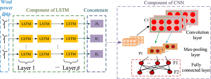
FIGURE 1. The LSTM-CNN joint prediction model.

In the first stage, the LSTM captures the temporal correlation in the data that has been preprocessed. Specifically, the processed power data of n wind turbines goes into n LSTM modules and each LSTM model is set to β layer. Each LSTM outputs a value. After concatenating and processing, the corresponding output values of each turbine are put into a two-dimensional matrix $W_p$ according to the location of the wind turbines.

In the second stage, the CNN is used to extract the spatial correlation stored in the matrix $W_p$. Starting from the input layer of CNN, the spatial features in the matrix $W_p$ are captured by the convolution kernel to obtain a new feature map. The CNN will gradually extract the spatial information of the spatial power matrix after multiple convolution-pooling layer structures and output a one-dimensional vector in the final output layer as the actual output of the model. In this study, Rectified Linear Unit (ReLU) is selected as the activation function of the convolutional layer. As an unsaturated nonlinear function that can accelerate the convergence rate during training, ReLU can significantly improve the performance of CNN. The definition of ReLU is as follows:

$g\left(x\right)=\left\{\begin{array}{c}x,x\ge 0\\ 0,x<0\end{array}\right\}(4)$

Algorithm Training

After establishing the joint model, a single loss function is used for end-to-end training. Because the power prediction can be regarded as a regression problem, the prediction goal is to minimize the error differentials between the model’s output sequence and the true value. Therefore, the mean squared error (MSE) is selected as the loss function for model training, and its definition as follows:

$L=\frac{1}{N}{\displaystyle \sum }_{i=1}^N{\left(Y_p-\widehat{Y_p}\right)}^2(5)$

Where, $L$ is the loss function, $N$ is the total number of samples, $\widehat{Y_p}$ and $Y_p$ are the predicted and true values, respectively.

The back-propagation rule and stochastic gradient descendant algorithm are adopted to train the entire network. The algorithms can automatically learn the rules of the network parameters to optimize the entire network, so that the output of the model can be closer to the true value. The error differential propagation starts from the last fully connected layer of the model through, i.e., propagating in the inverse time direction. Subsequently, the propagated error differentials pass through the entire CNN to the LSTM, and then backward propagate to the input layer of the entire model. In this way, the parameters of the model are iteratively updated according to the error differentials, and finally the optimal parameters are learned. In this process, the parameters of the entire model are supervised by the gradient-based training method. The prediction model integrates the learned spatiotemporal information and finally achieves the purpose of power prediction using the spatiotemporal correlation.

Experimental Validations

Data Description

In this experiment, the SCADA data of 34 wind turbines at Guishan offshore wind farm in China within 1 wk of November 2019 was collected and used. The distribution of the wind farm is shown in Figure 2. All wind turbine models are exactly the same, and the time resolution of the data is 1 min. The single data set for the experiment contains a total of 20,160 frames. The data set is divided into three mutually exclusive subsets: training set, test set, and verification set. The training set and the test set account for the first 60 and 20% of the data set, respectively. The last 20% of the data set is used to evaluate the model’s generalization ability. In order to achieve better results for the model, eight wind turbines with the closing distribution position in the wind farm are selected as the research objects, which are # 17, # 18, # 19, # 20, # 23, # 24, # 25, # 26, respectively.

FIGURE 2

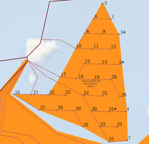
FIGURE 2. Distribution map of Guishan offshore wind farm in Zhuhai.

Model Parameter Setting

First of all, a truncated normal distribution is used when initializing network parameters. Meanwhile, the Adam algorithm is selected as the optimization function of the model, of which the learning rate is set to 0.01, and the iteration is 100 times.

In the model, the length of the sliding window to obtain the input sequence (i.e., α) directly affects the effect of LSTM on the temporal correlation extraction of historical sequence data. If α is too small, the time features included in the input sequence are insufficient, which affect the prediction accuracy of the model. If α is too large, it makes the structure of the model complicated and training more difficult. Considering the above two aspects comprehensively, and through a large number of experimental tests, α is finally selected to be 20.

Then, the number of LSTM models is set to 8, which is the same as the quantity of the selected wind turbines. In order to extract the temporal features, the number of LSTM layers β is set to 2. In the merge processing module of the joint model, the output data of #17, #18, #19, #20 are put on the first row of $W_p$, and the output data of #23, #24, #25, #26 on the second row. By doing so, a two-dimensional spatial matrix $W_p$ is obtained. Since $W_p$ is just a matrix of (2, 4) shape, the contained features are not complicated, so only one convolution layer C1 is used in the CNN model.

Lastly, the convolution kernels’ number of the convolutional layer is set to 32. Each convolution kernel is a two-dimensional matrix with a height and width of 2. The edge of the input image is filled with a size of 1, and the input is convolved with a step size of 1. The first layer of convolutional layer C1 outputs a convolutional image of size (2, 4, 32), which is used as the input of the pooling layer P1. In this study, the maximum pooling method is selected, that is, the P1 layer is the Max Pooling layer, the pooling core size of P1 is set to 2 × 2, and the step size is 2. When the output of C1 reaches P1, P1 outputs a result of shape (1, 2, 32). Subsequently, pass it to the fully connected layers F1 and F2. The F1 input dimension is set to 1 * 2 * 32 = 64, the output dimension is set to 100, and the F2 input dimension and output dimension are set to 100 and 8, respectively.

Experimental Results

In order to verify the comprehensive performance of the established model, three algorithms are selected and developed for comparison, including Support Vector Machine (SVM), LSTM and CNN. The three models have been trained separately, and the models having the best performance are saved. The data of four wind turbines, # 17, # 19, # 23 and # 25, are selected to discuss, and the predicted wind power of the four models are obtained.

The predicted value and the real values of the 2 h are plotted in Figure 3. As seen from Figure 3, the prediction curve of the LSTM-CNN joint model is closer to the true value than the other three prediction algorithms. To be specific, the LSTM effectively extracts the time correlation, and it also has good prediction performance. By comparison, the CNN and SVM perform poorly. The reason is that, when facing the problem of power prediction of multiple wind turbines, the CNN can effectively capture the spatial features of the data, but it does not take the temporal correlation into account. Similarly, the LSTM has excellent performance when facing timing prediction problems, but ignores the spatial features. Since the SVM only uses the global spatial and temporal information in the data, its prediction preciseness is noticeably lower than the three counterparts.

FIGURE 3

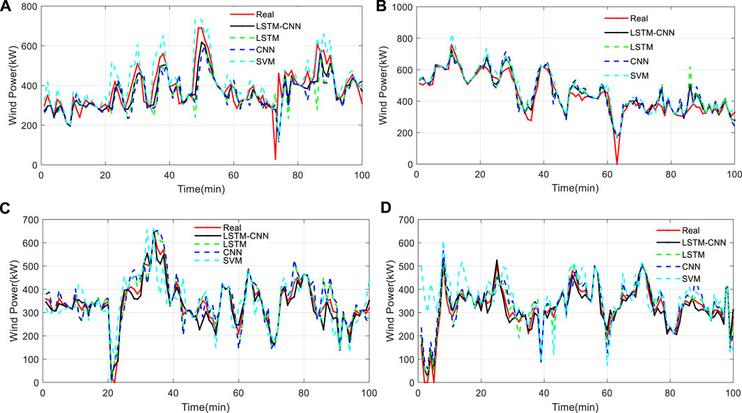
FIGURE 3. Two-hour power prediction results for wind turbines: (A) #17; (B) #19; (C) #23; (D) #25.

To further evaluate the performance of different prediction methods, the widely used performance indicators are used and calculated: root mean squared error (RMSE) and mean absolute error (MAE), and MSE. The data of the last 2 h in the prediction data obtained from the test set is selected and divided into four steps to evaluate the four models. That is, let k be the number of steps, and obtain 30-min prediction data at each step to compare with the comparison algorithm. The results of performance indicators are shown in Figure 4, from which the observations can be summarized as two aspects. On the one side, with the increase of the prediction step, the prediction effect of each model all decreases. Specifically, the SVM declines fastest, followed by CNN, LSTM, and the last comes the LSTM -CNN joint model. On the other side, for the four prediction models, the MSE, RMSE, and MAE of the LSTM-CNN joint model are lower than the other three models, and the LSTM-CNN joint model has the best performance when facing the problem of prediction for power of multiple wind turbines at different locations.

FIGURE 4

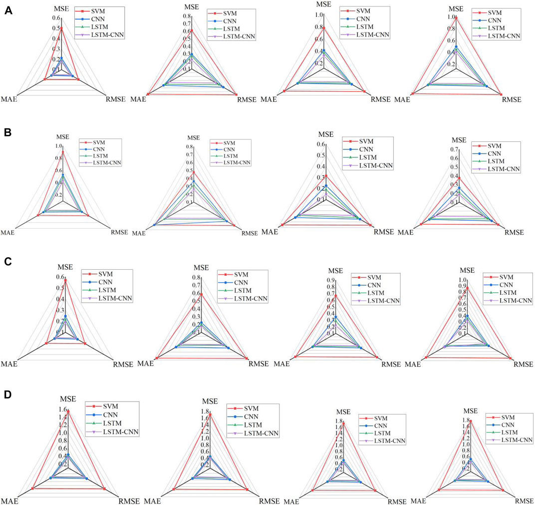
FIGURE 4. Prediction results for the four wind turbines under different prediction steps: (A) step = 1; (B) step = 2; (C) step = 3; (D) step = 4.

To sum up, the proposed LSTM-CNN joint model making full use of high-level spatiotemporal features, is capable of simultaneously predicting the power of multiple wind turbines in terms of its two-stage structure. The input data of LSTM is a one-dimensional array of a specific length and multiple LSTMs are simultaneously operated to complete the extraction of the temporal features of the wind turbines in different locations, so that the temporal correlation in the time series can be fully extracted. After extracting time features by LSTM, a spatial power matrix is concatenated, in which the spatial features are captured by CNN, and thus the prediction task is successfully fulfilled.

Conclusion

The proposed prediction model is based on the modeling idea of “capturing temporal dependence first and then extracting spatial features.” Composed of LSTM and CNN, the model was trained end-to-end by a unified loss function. The trained model can extract high-level spatiotemporal features from the historical power data of wind turbines, so as to achieve the purpose of simultaneously predicting the power of wind turbines at different locations. The measured data of an offshore wind farm in China was used for simulation experiments and the real values were compared with the predicted values of the model. The comparison results showed that the proposed method has more excellent performance than the existing prediction methods, such as LSTM, CNN, and SVM. With the proposed model, it is possible to precisely predict the wind power of multiple wind turbine within a wind farm with the regular layout. On this basis, it can be performed the accurate power scheduling, which is the future research direction.

Data Availability Statement

The raw data supporting the conclusions of this article will be made available by the authors, without undue reservation.

Author Contributions

XC: Methodology, Software, Validation, Writing- Original draft preparation, Writing- Reviewing and Editing. XZ: Methodology, Writing- Original draft preparation. MD: Methodology, Supervision. LH: Conceptualization, Supervision. YG: Test, Validation, Investigation. SH: Test, Writing-Reviewing and revise grammar and correct expression.

Funding

This work was supported in part by the Major Science and Technology Projects in Anhui Province under Grant 202003a05020019, and in part by the Comprehensive Research Facility for Fusion Technology under Grant 2018-000052-73-01-001228.

Conflict of Interest

The authors declare that the research was conducted in the absence of any commercial or financial relationships that could be construed as a potential conflict of interest.

Publisher’s Note

All claims expressed in this article are solely those of the authors and do not necessarily represent those of their affiliated organizations, or those of the publisher, the editors and the reviewers. Any product that may be evaluated in this article, or claim that may be made by its manufacturer, is not guaranteed or endorsed by the publisher.

References

Hazari, M., Mannan, M., Muyeen, S., Umemura, A., Takahashi, R., and Tamura, J. (2017). Stability Augmentation of a Grid-Connected Wind Farm by Fuzzy-Logic-Controlled DFIG-Based Wind Turbines. Appl. Sci. 8, 20. doi:10.3390/app8010020

CrossRef Full Text | Google Scholar

Hochreiter, S., and Schmidhuber, J. (1997). Long Short-Term Memory. Neural Comput. 9 (8), 1735–1780. doi:10.1162/neco.1997.9.8.1735

PubMed Abstract | CrossRef Full Text | Google Scholar

Jinfu, C., Qiaomu, Z., Dongyuan, S., et al. (2019). A Multi-step Wind Speed Prediction Model for Multiple Sites Leveraging Spatio-Temporal Correlation. Proc. CSEE 39 (17), 2093–2105. doi:10.13334/j.0258-8013.pcsee.180897

Google Scholar

Lecun, Y., Bengio, Y., and Hinton, G. (2015). Deep Learning. Nature 521 (7553), 436–444. doi:10.1038/nature14539

PubMed Abstract | CrossRef Full Text | Google Scholar

Liu, Bo., He, Zhijia., and Jin, Hao. (2016). Current Status and Development Trend of Wind Power Generation. J. Northeast Dianli Univ. 36 (02), 7–13. doi:10.19718/j.issn.1005-2992.2016.02.002

Google Scholar

Seo, S., Oh, S.-D., and Kwak, H.-Y. (2019). Wind Turbine Power Curve Modeling Using Maximum Likelihood Estimation Method. Renew. Energ. 136 (JUN), 1164–1169. doi:10.1016/j.renene.2018.09.087

CrossRef Full Text | Google Scholar

Song, D., Chang, Q., Zheng, S., Yang, S., Yang, J., and Hoon Joo, Y. (2021a). Adaptive Model Predictive Control for Yaw System of Variable-Speed Wind Turbines. J. Mod. Power Syst. Clean. Energ. 9 (1), 219–224. doi:10.35833/mpce.2019.000467

CrossRef Full Text | Google Scholar

Song, D., Zheng, S., Yang, S., Yang, J., Dong, M., Su, M., et al. (2021b). Annual Energy Production Estimation for Variable-Speed Wind Turbine at High-Altitude Site. J. Mod. Power Syst. Clean. Energ. 9 (3), 684–687. doi:10.35833/MPCE.2019.000240

CrossRef Full Text | Google Scholar

Yang, B., Wang, J., Zhang∗, X., Yu, T., Yao, W., Shu, H., et al. (2020). Comprehensive Overview of Meta-Heuristic Algorithm Applications on Pv Cell Parameter Identification. Energ. Convers. Manage. 208, 112595. doi:10.1016/j.enconman.2020.112595

CrossRef Full Text | Google Scholar

Yang, B., Yu, T., Zhang∗, X., Li, H., Shu, H., Sang, Y., et al. (2019a). Dynamic Leader Based Collective Intelligence for Maximum Power point Tracking of PV Systems Affected by Partial Shading Condition. Energ. Convers. Manage. 179, 286–303. doi:10.1016/j.enconman.2018.10.074

CrossRef Full Text | Google Scholar

Yang, B., Zhong, L., Zhang, X., Shu, H., Yu, T., Li, H., et al. (2019b). Novel Bio-Inspired Memetic Salp Swarm Algorithm and Application to MPPT for PV Systems Considering Partial Shading Condition. J. Clean. Prod. 215, 1203–1222. doi:10.1016/j.jclepro.2019.01.150

CrossRef Full Text | Google Scholar

Yang, J., Fang, L., Song, D., Su, M., Yang, X., Huang, L., et al. (2021). Review of Control Strategy of Large Horizontal‐axis Wind Turbines Yaw System. Wind Energy 24 (2), 97–115. doi:10.1002/we.2564

CrossRef Full Text | Google Scholar