High Resolution 3-D Simulations of Venting in 18650 Lithium-Ion Cells

1 Introduction

Lithium-ion batteries (LIB) are a prevailing energy storage device widely used in mobile applications like portable electronic devices, electrical vehicles and aircraft because of their high energy and power density (Feng et al., 2018; Wang et al., 2019). However, safety remains a challenge for LIBs, especially with increasing power and energy density at the module- and system-level. The fire hazard of LIBs is driven by the risk of thermal runaway, during which a large quantity of heat and gas is produced by a series of exothermal reactions, including: decomposition of the solid electrolyte interphase (SEI) layer, reaction of anode with electrolyte, cathode decomposition, electrolyte decomposition, and others (Kim et al., 2007). The high level of heat and gas generation rates during thermal runaway cause the temperature and pressure inside the cell increase, nearly instantaneously. Common 18650 format LIB cells have a safety vent mechanism built into the positive terminal cap and when the internal pressure of the cell increases to the vent activation pressure, the safety vent opens releasing flammable and toxic gases as well as electrolyte vapors (Nedjalkov et al., 2016). The vented flammable gas may ignite, causing fire and increasing risk of thermal runaway propagation within a multi-cell module or system (Wang et al., 2012). Developing methods, either numerical or experimental, to investigate the flow field during venting can help provide new insights into the combustion and heat transfer during propagating failures.

The following information is needed for development of models which are capable of simulating a full thermal runaway, with effects of combustion and heat transfer resulting from vented gases included: decomposition reaction sequence, kinetic model and parameters for each reaction, heat and gas generation amounts associated with each reaction, and composition of gases emerging from the cell during venting. Significant work has been accomplished in developing the reaction sequence, kinetic model and parameters, and heat generation amounts. The classical paper by Hatchard et al. laid the groundwork for thermal abuse models of Li-ion cells using three decomposition reactions: SEI decomposition, reaction of anode and electrolyte, and cathode decomposition (Hatchard et al., 2001). Since then, many studies have built on the original model framework to account for additional reactions (Kim et al., 2007; Ren et al., 2018; Xu et al., 2018), to consider different cell chemistries (Peng and Jiang, 2016; Dong et al., 2018; Bugryniec et al., 2020), to account for aging (Prada et al., 2012; Abada et al., 2018; Larsson et al., 2018), to investigate different thermal management strategies (Chen et al., 2016; Lopez et al., 2016; Bugryniec et al., 2020), and to account for gas generation from decomposition reactions (Coman et al., 2017; Ostanek et al., 2020).

Relatively few studies have considered the effects of venting in numerical thermal abuse models. Coman et al. (Coman et al., 2016) developed a thermal abuse model of an 18650 cylindrical cell which considered the effects of electrolyte evaporation and venting. The authors reported that time-to-runaway is not captured accurately when endothermic effects such as evaporation of electrolyte and enthalpy carried away from the cell by ejecta are neglected. Coman et al. (Coman et al., 2017) then included gas generation from the SEI decomposition reaction, which contributes to pressure buildup in the cell along with evaporation of electrolyte, and found that time-to-venting was captured more accurately. The evaporation model of Coman et al. (Coman et al., 2017) assumed the electrolyte is in a state of vapor-liquid-equilibrium (VLE) prior to venting. Our previous work (Ostanek et al., 2020; Parhizi et al., 2021) built upon the lumped model approach and included a model for non-VLE evaporation after venting using a constant-rate and decaying-rate drying model. For oven tests and other slow heating abuse tests, the cell temperature decreases after vent-activation because of the heat absorbed during non-VLE evaporation. Mao et al. (Mao et al., 2021) considered the reacting flow after venting and developed a lumped model to estimate the flame height for flow emerging from an Nickel Cobalt Manganese (NCM) chemistry 18650 cell. The model assumes that the safety vent is a circular orifice and calculates the vent gas velocity assuming the isentropic flow rate.

The venting of gases emerging from Li-ion cells, and subsequent combustion, has important effect on the thermal runaway propagation within a module or system. Combustion of vented gases increase heat transfer to neighboring cells by impingement and thermal radiation. Walker et al. (Walker et al., 2019) investigated the fraction of the energy released through cell case and the ejecta and vented gases during thermal runaway. The results showed that the energy released through the ejecta and gases was larger than that released by conduction through the cell case for four types of Li-ion caps (Samsung 18650-3Q, LG 18650-MJ1, 3.35 Ah LG 18650, and MOLiCEL 18650-J). Using LG 18650 MJ1 as an example, 78.3% of the total energy released in thermal runaway (74.9 kJ) was transferred by the ejecta and vented gases. Zhong et al. (Zhong et al., 2018) studied the thermal runaway propagation in an 18650 LIB module with 3 × 3 cells. If the cells were displaced with 4 mm distance to each other, the thermal runaway can still propagate to the surrounding cells by the thermal shock created by the flame of the vented gases. Archibald et al. (Archibald et al., 2020) found that the thermal runaway propagation in the 10 × 10 Ah module was faster than that in 10 × 5 Ah module. The larger thermal runaway propagation speed was due to preheating of the unfailed cells by the high temperature vented gas generated from failed cells. The higher chamber temperature produced by the vented gas also decreased the heat loss of cells. Cheng et al. (Cheng et al., 2019) used video analysis to study the thermal runaway procedure of a LIB module with 12 commercial NCM prismatic cells. The thermal runaway propagation was attributed to heat conduction between cells as well as convection and radiation caused by combustion of the vented gas. The flames ignited the wire harness of cells on the other side of the module and initiated thermal runaway in those cells. Mishra et al. (Mishra et al., 2021) investigated the impact of vent gas flow on thermal runaway propagation in a 25-cell module. The primary heat transfer mechanism considered in this study was the flow of hot gases from a failed cell impinging on neighboring cells and nearby surfaces. The cell-to-cell spacing, overhead gap spacing, and location of the vent hole had significant effect on thermal runaway propagation.

Although venting and combustion play an important role in module-level protection, there is a substantial lack of literature on numerical modeling of the external flow phenomena. Existing studies which consider venting and combustion typically simplify the vent geometry to a circular orifice which may not capture the spatial distribution and velocity fields of vented gases within the module. The present work investigates the flow field during venting of an 18650 LIB cell using a three-dimensional (3-D) CFD model based on highly detailed cap geometries. The ensemble-averaged flow field was simulated using Reynolds-averaged Navier-Stokes (RANS) simulations. Model benchmarking and a mesh sensitivity analysis were conducted for a sharp-edge orifice. From a series of RANS simulations across a range of pressure ratios, sharp-edge orifice equivalent areas were calculated for each battery cap and compared with experimental data. The restriction imposed by each vent cap was quantified using the equivalent sharp-edge orifice flow area. The unsteady flow field was then analyzed using scale-resolving simulations (SRS). Mean and fluctuating velocity distributions obtained from SRS were investigated and the turbulent structures emerging from the vent were visualized.

2 Methods

2.1 RANS CFD Model for LIB Caps

CFD simulations were conducted using the commercial software, Fluent® version 19.2 (ANSYS, 2019b; a). The CFD model is based on the finite volume method, which solves the governing equations for compressible flow through the vent cap assembly: continuity, momentum, energy, turbulence kinetic energy, and turbulence dissipation rate (ANSYS, 2019a). The continuity equation is:

$\frac{\partial \rho }{\partial t}+\frac{\partial }{\partial x_i}\left(\rho {\overline{u}}_i\right)=0(1)$

where ρ is the fluid density and ${\overline{u}}_i$ is the mean velocity vector. Note that the overbar indicates mean quantities resulting from the ensemble-averaging procedure. The conservation of momentum equation is:

$\frac{\partial }{\partial t}\left(\rho {\overline{u}}_i\right)+\frac{\partial }{\partial x_j}\left(\rho {\overline{u}}_i{\overline{u}}_j\right)=-\frac{\partial \overline{p}}{\partial x_i}+\frac{\partial }{\partial x_j}\left[\mu \left(\frac{\partial {\overline{u}}_i}{\partial x_j}+\frac{\partial {\overline{u}}_j}{\partial x_i}-\frac{2}{3}{\delta }_{ij}\frac{\partial {\overline{u}}_l}{\partial x_l}\right)\right]+\frac{\partial }{\partial x_j}\left(-\rho \overline{u_i^{\prime }{u}_j^{\prime }}\right)(2)$

where μ is the molecular viscosity, δ_ij is the Kronecker delta, $\overline{p}$ is the mean pressure, and $-\rho \overline{u_i^{\prime }{u}_j^{\prime }}$ is the Reynolds stress tensor. The conservation of energy equation is:

$\frac{\partial \rho \overline{E}}{\partial t}+\frac{\partial }{\partial x_i}\left(u_i\left(\rho \overline{E}+\overline{p}\right)\right)=\frac{\partial }{\partial x_j}\left(\left(\lambda +{\lambda }_T\right)\frac{\partial \overline{T}}{\partial x_j}\right)(3)$

where $\overline{T}$ is mean temperature, $\overline{E}$ is mean energy ($\overline{h}-\frac{\overline{p}}{\rho }+\frac{{\overline{U}}^2}{2}$), λ is thermal conductivity, and λ_T is the turbulent thermal conductivity. The conservation of turbulence kinetic energy equation is:

$\frac{\partial }{\partial t}\left(\rho k\right)+\frac{\partial }{\partial x_i}\left(\rho k{\overline{u}}_i\right)=\frac{\partial }{\partial x_j}\left[\left(\mu +\frac{{\mu }_T}{{\sigma }_k}\right)\frac{\partial k}{\partial x_j}\right]+G_k-\rho \epsilon -Y_M(4)$

where $k$ is turbulent kinetic energy, μ_T is the turbulent viscosity, σ_k is the turbulent Prandtl number for turbulence kinetic energy, G_k is the generation of turbulence kinetic energy due to the mean velocity gradients, $\epsilon$ is turbulence dissipation rate, and Y_m is the contribution of the fluctuating dilatation in compressible turbulence to the overall dissipation rate. The conservation of turbulence dissipation rate equation is:

$\frac{\partial }{\partial t}\left(\rho \epsilon \right)+\frac{\partial }{\partial x_i}\left(\rho \epsilon {\overline{u}}_i\right)=\frac{\partial }{\partial x_j}\left[\left(\mu +\frac{{\mu }_T}{{\sigma }_{\epsilon }}\right)\frac{\partial \epsilon }{\partial x_j}\right]+\rho C_{1}S\epsilon -\rho C_2\frac{{\epsilon }^2}{k+\sqrt{\nu \epsilon }}(5)$

where C₂ is constant, $C_1=\max \left[0.43,\frac{\eta }{\eta +5}\right], \eta =S\frac{k}{\epsilon }, S=\sqrt{2S_{ij}{S}_{ij}}$, $S_{ij}=\frac{1}{2}\left(\frac{\partial {\overline{u}}_j}{\partial x_i}+\frac{\partial {\overline{u}}_i}{\partial x_j}\right)$, and σ_ε is the turbulent Prandtl number for turbulence dissipation rate.

Four commercial LIB vent cap assemblies were considered in this paper: MTI, LG MJ1, K2, and LG M36. All four vent caps are used in 18650 format cylindrical Li-ion cells (18 mm diameter, 65 mm length). The MTI vent cap assembly was purchased as an individual component from the manufacturer, while the remaining 3 cells were extracted from live Li-ion cells following the procedure of our previous work (Li et al., 2020b). The LG MJ1 cap was extracted from an LG INR18650 MJ1 cell, the K2 cap was extracted from a K2 LFP18650E-1500-03 cell, and the LG M36 cap was extracted from an LG INR18650 M36 cell. The nominal voltage of the LG INR18650 MJ1 cell is 3.6 V, the nominal capacity is 3.5 Ah, and the electrodes are LiNiMnCoO₂-graphite. The nominal voltage of the K2 LFP18650E-1500-03 cell is 3.2 V, the nominal capacity is 1.5 Ah, and the electrodes are LiFePO₄-graphite. The nominal voltage of the LG INR18650M36 cell is 3.63 V, the nominal capacity is 3.6 Ah, and the electrodes are LiNiMnCoO₂-graphite.

After extracting the vent cap assemblies from the commercial cells, computed tomography (CT) scans were conducted following the procedure of our previous work (Li et al., 2020b). From the CT scans, which are publicly available for download (Stoll et al., 2020b; a; 2021a; b), detailed 3-D geometric models of the caps in a vent activated state were developed for use in CFD simulations. An isometric view of the geometric model for each commercial LIB vent cap assembly is shown in Figure 1.

FIGURE 1

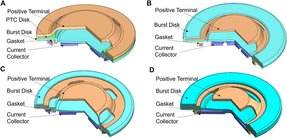
FIGURE 1. Detailed 3-D geometric model with vent cap assembly components listed for the: MTI cap (A), LG MJ1 cap (B), K2 cap (C), and LG M36 cap (D).

The CFD model was developed using the detailed vent cap geometric models shown in Figure 1. The computational domain, boundary conditions, and mesh used for 3-D simulations of flow through the vent caps are shown in Figure 2. The computational domain was designed to emulate an experimental setup that was developed previously to measure discharge coefficients of commercial LIB caps (Li et al., 2020a). The apparatus uses a flat plate with a rounded inlet which holds the LIB cap specimen. The flat plate also serves as a divider between upstream and downstream chambers. The pressure ratio across the cap is set by adjusting the pressure in the two chambers. The computational domain in Figure 2A emulates the experimental apparatus but consists of only the fluid region. In other words, the solid parts (LIB cap and separator plate) were subtracted from the full domain, leaving just the fluid region as shown in Figure 2B. A hemispherical surface having radius of 180 mm was assigned a pressure outlet boundary condition. Impermeable, no-slip, and adiabatic wall boundary conditions were assigned to the surfaces of the LIB cap and the fixture plate. A smaller hemispherical surface having radius of 45 mm was assigned as a pressure inlet boundary condition.

FIGURE 2

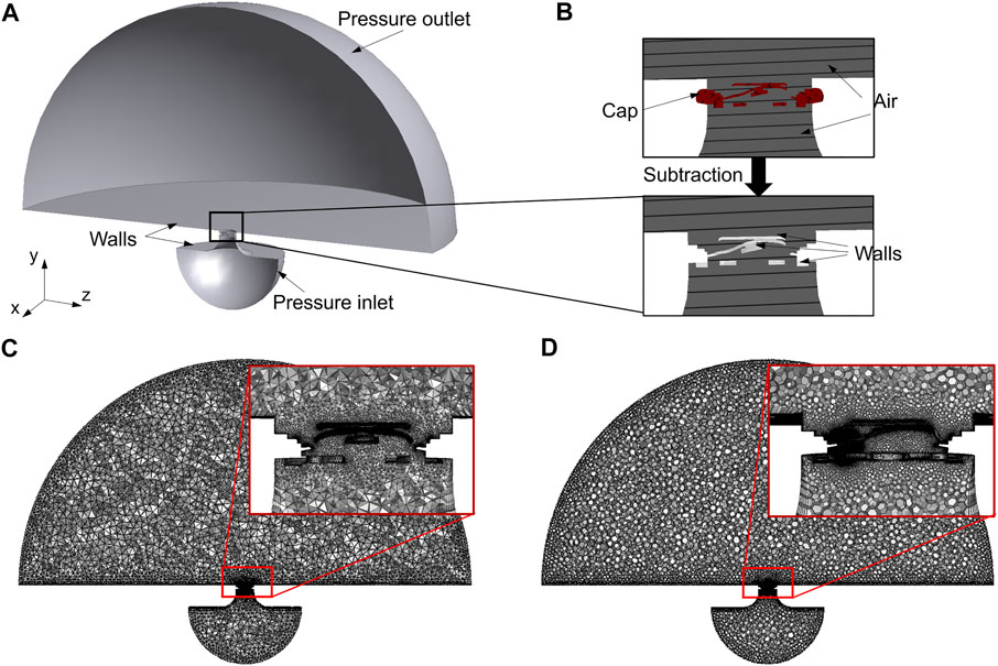
FIGURE 2. Computational domain and boundary conditions for RANS simulations of flow through LIB caps (A), schematic of the Boolean-subtraction procedure to obtain the fluid-only computational domain (B), fine tetrahedral mesh as viewed normal to the z-axis (C), and fine polyhedral mesh as viewed normal to the x-axis (D).

The working fluid was assumed to be single-phase, dry air. The total pressure at the inlet was varied such that P₁/P₂ ranged from 1.2 to 8. Total temperature at the inlet was T₁ = 300 K. The outlet total pressure was set to P₂ = 101.3 kPa. It was assumed the incoming flow was straightened and conditioned, with a turbulence intensity of 0.5% and turbulent length scale of 5 mm.

Recommended solver settings from the Fluent^® version 19.2 theory manual were used to solve the single-phase, compressible, turbulent jet flow issuing through a restriction (ANSYS, 2019a). The pressure-based coupled algorithm and the realizable k-ε turbulence model with scalable wall functions were used. Fluid properties were modeled using the ideal gas equation of state model, and temperature-dependent polynomials were used for transport properties where specific heat capacity at constant pressure is shown in Eq. 6, molecular viscosity is shown in Eq. 7, and thermal conductivity is shown in Eq. 8.

$c_p=-1.14\times {10}^{-13}{T}^5+7.66\times {10}^{-10}{T}^4-1.92\times {10}^{-6}{T}^3+2.17\times {10}^{-3}{T}^2-8.82\times {10}^{-1}T+1.12\times {10}^3(6)$

$\mu =2.17\times {10}^{-21}{T}^5-1.52\times {10}^{-17}{T}^4+4.22\times {10}^{-14}{T}^3-6.35\times {10}^{-11}{T}^2+7.56\times {10}^{-8}T+5.24\times {10}^{-7}(7)$

$\lambda =7.43\times {10}^{-21}{T}^5-4.92\times {10}^{-17}{T}^4+4.76\times {10}^{-12}{T}^3-2.92\times {10}^{-8}{T}^2+9.05\times {10}^{-5}T+9.92\times {10}^{-4}(8)$

Second-order upwind discretization was used for discretization of advection terms for improved accuracy relative to the first-order upwind scheme (ANSYS, 2019a). The simulations were carried out until the normalized residuals were less than the default values of 1E-3 for continuity, momentum, and turbulent transport equations and 1E-6 for the energy equation (ANSYS, 2019b).

Two different unstructured meshing approaches were used to discretize the computational domain: tetrahedral elements and polyhedral elements. Tetrahedral meshes were generated using the meshing utility with ANSYS Workbench (ANSYS, 2019c). Polyhedral meshes were obtained by conversion of the tetrahedral meshes using the polyhedral conversion utility within ANSYS Fluent (ANSYS, 2019b). A mesh sensitivity was conducted using coarse, medium, and fine meshes for both tetrahedral and polyhedral meshes. Mesh constraints included a global element size of: 5 mm for the coarse mesh, 3.5 mm for the medium mesh, and 2.5 mm for the fine mesh. All meshes were generated using: global element growth rate of 1.2, edge proximity capture with a minimum element size of 80 μm, curvature capture with a minimum element size of 100 μm, and wall-adjacent inflation layers having five layers with a transition ratio of 0.272. Examples of fine meshes using tetrahedral and polyhedral elements are shown in Figures 2C,D, respectively. Both Figures 2C,D show the mesh for the LG MJ1 cap. Figure 2C shows the plane which is normal to the z-axis and Figure 2D shows the plane normal to the x-axis.

2.2 SRS CFD Model for LG MJ1 Cap

The scale-resolved simulations (SRS) technique, specifically the stress-blended eddy simulation (SBES) turbulence model, was used to simulate unsteady flow through the LG MJ1 cap. The geometric model and computational domain were modified from the domain used in RANS simulations. Instead of a domain which replicated the experimental setup for discharge coefficient measurement, a new domain was created which includes an 18650 cell surrounded by an air space, as shown in Figure 3A. The element sizing constraints within the vent cap were the same as that of the fine polyhedral mesh described in section 2.1. The mesh density outside the cell near the vent holes was refined using conical regions placed above the vent holes. The mesh density was adjusted by using three different conical regions with progressively increasing element size, 0.2 mm to 0.5 mm to 0.8 mm, moving from the inner to outer cones, respectively. The mesh density in the three conical regions is shown in Figure 3B.

FIGURE 3

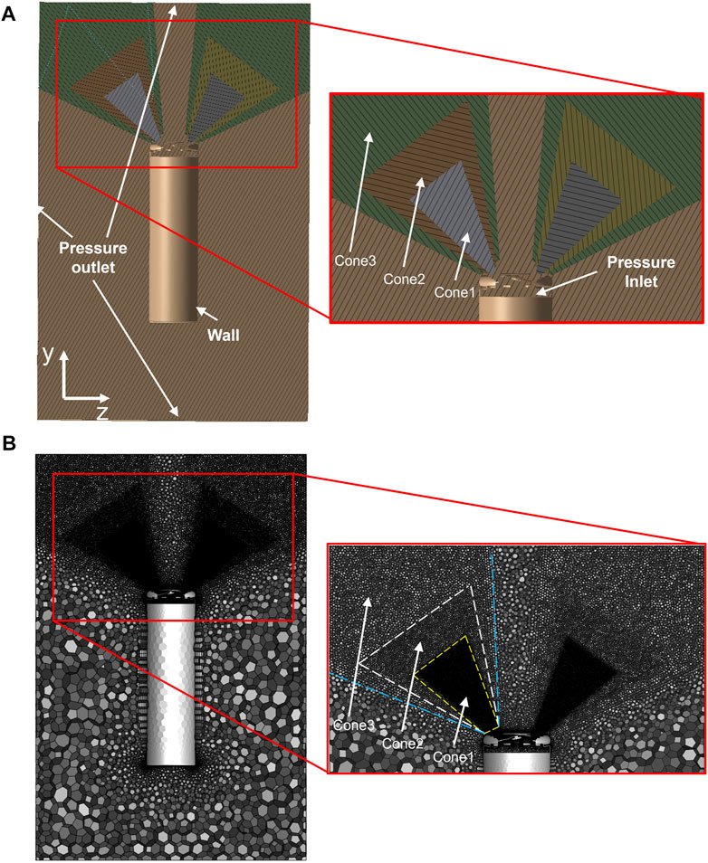
FIGURE 3. Cross-sectional view showing the geometry (A) and mesh (B) of computational domain and boundary conditions for SRS simulations of flow through the LG MJ1 cap.

The pressure inlet boundary condition was set in the plane which would be located below the vent cap, as shown in Figure 3A. The outer surfaces of the cylindrical domain of the fluid were assigned pressure outlet boundaries to represent a single cell sitting in a quiescent environment. The wall surfaces of the cap and cell case were assigned no-slip, adiabatic, and impermeable boundary conditions. The time step for the simulation was set to 1E-6 s. The same solver settings in section 2.1 were used: pressure-based coupled algorithm, temperature-dependent polynomial functions for transport properties, and ideal gas equation of state. Advection terms in the momentum equation were discretized using the default setting for the SBES model: bounded, second-order differencing scheme (ANSYS, 2019b).

3 Results and Discussion

3.1 Sharp-Edge Orifice Benchmarking

The CFD procedures described in section 2.1 were implemented for a benchmark case of compressed air flowing through a sharp-edge orifice. The model setup and results of the benchmarking case are shown in the Supplementary Material. A mesh sensitivity analysis was conducted for the benchmarking case, using the same global element sizing and inflation layer settings as those used for the LIB cap simulations. Results of the benchmarking cases agreed with literature data and, thus, the CFD solution procedure was considered suitable for the LIB cap simulations.

3.2 RANS Simulations for LIB Caps

A series of RANS CFD simulations were conducted to analyze the ensemble-averaged flow field emerging from LIB vent caps under a range of pressure ratios. First, a mesh sensitivity analysis was conducted for the RANS CFD model. Next, the discharge coefficients for the LIB caps were calculated over a range of pressure ratios. The discharge coefficients were compared to previous experimental data and also used to compare the flow restriction imposed by each vent cap. Finally, details of the simulated flow field, including Mach number and turbulent viscosity ratio distributions, were analyzed and compared for each of the four battery caps.

3.2.1 Mesh Sensitivity of Mach Number Distribution Analysis

A mesh sensitivity analysis was conducted for the LG MJ1 vent cap. The sensitivity analysis was conducted for the coarse, medium and fine meshes for the two element types, tetrahedral and polyhedral. For tetrahedral elements the coarse mesh had ∼4.93E6 elements, the medium mesh had ∼7.69E6 elements, and the fine mesh had ∼12.6E6 elements. The polyhedral mesh sizes were: coarse ∼2.35E6 elements, medium ∼3.14E6 elements, and fine ∼4.14E6 elements.

The velocity magnitude, represented by Mach number, was extracted along two different lines for a flow simulation with a pressure ratio of P₁/P₂ = 7: one aligned with the jet and one extending across one of the vent holes in the horizontal (transverse) direction. Along the jet axis, as shown in the inset of Figure 4A, the Mach number distribution showed little sensitivity to the mesh refinement level. In particular, the simulation results for the three polyhedral meshes showed very little change between the three mesh refinements. In Figure 4B, the Mach number distribution also showed little sensitivity to the mesh refinement level. At this pressure ratio, the maximum Mach number was just over 2.0.

FIGURE 4

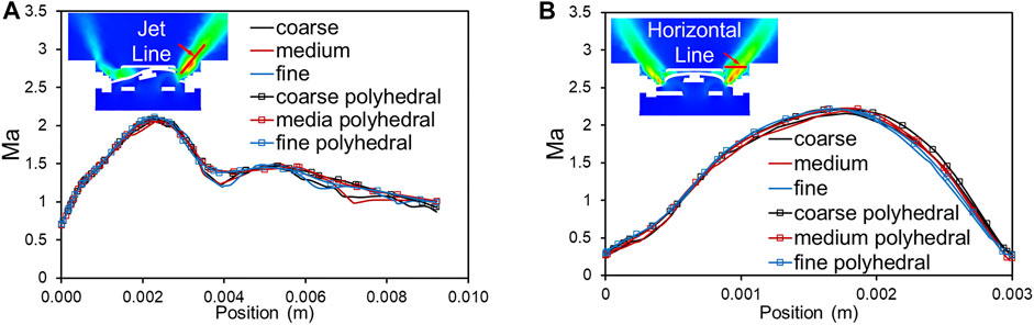
FIGURE 4. Mesh sensitivity analysis conducted on the LG MJ1 cap at P₁/P₂ = 7 showing Mach number along the jet line (A) and along the horizontal line across the vent opening (B).

In addition to comparing the local Mach number distribution, the mass flow rate through the cap was monitored for the P₁/P₂ = 7 flow simulation. The simulated mass flow rate obtained with coarse, medium, and fine meshes using tetrahedral elements had less than 0.4% variation. The simulated mass flow rate obtained with coarse, medium, and fine meshes using polyhedral elements had less than 0.1% variation. The difference in the mass flow rate between the tetrahedral and polyhedral meshes was 0.77% for the coarse mesh, 0.62% for the medium mesh, and 0.97% for the fine mesh.

Polyhedral elements have the following advantages relative to tetrahedral elements: improved mesh quality, faster convergence, and lower overall mesh count (ANSYS, 2019b). Considering these advantages, and the less than 0.97% difference in flow rate with the defined mesh sizing parameters, polyhedral elements with the fine mesh density were used for discharge coefficient comparison and flow field analysis for all four caps. Using the fine polyhedral mesh at a pressure ratio of P₁/P₂ = 7, the average wall y + values for the MTI, LG MJ1, K2, and LG M36 caps model were 8.94, 9.72, 14.51, and 13.64, respectively. The maximum wall y + values for the MTI, LG MJ1, K2, and LG M36 caps model were 77.80, 56.49, 64.8, and 140.36, respectively.

3.2.2 Sharp-Edge Orifice Equivalent Area Analysis: Models Compared to Experiments

The flow restriction of each cap was quantified by calculating a sharp-edge orifice equivalent area by a method of least squares fitting of discharge coefficients to those of a sharp-edge orifice. The discharge coefficient is the ratio of actual mass flow rate $\dot{m}$ through the restriction divided by the ideal, isentropic flow through the restriction, ${\dot{m}}_{ideal}$, (Li et al., 2020a), as shown in Eq. 9.

$C_d=\frac{\dot{m}}{{\dot{m}}_{ideal}}(9)$

The minimum flow area required to calculate ${\dot{m}}_{ideal}$ is difficult to determine for the LIB cap due to the complex geometry of the current collector plate, positive terminal plates, and deformed burst disk (Li et al., 2020a). The area appears in Eq. 10, for the ideal mass flow rate through a restriction:

${\dot{m}}_{ideal}=\{\begin{array}{cc}A{P}_1\sqrt{\frac{\gamma }{R{T}_1}{\left(\frac{2}{\gamma +1}\right)}^{\left(\gamma +1\right)/\left(\gamma -1\right)}}& \frac{P_2}{P_1}<{\left(\frac{2}{\gamma +1}\right)}^{\frac{\gamma }{\gamma -1}}\\ A{P}_1\sqrt{\frac{2\gamma }{R{T}_1\left(\gamma -1\right)}\left({\left(\frac{P_2}{P_1}\right)}^{2/\gamma }-{\left(\frac{P_2}{P_1}\right)}^{\left(\gamma +1\right)/\gamma }\right)}& \frac{P_2}{P_1}\ge {\left(\frac{2}{\gamma +1}\right)}^{\frac{\gamma }{\gamma -1}}\end{array}(10)$

where A is the flow area of the restriction, P₁ is the upstream stagnation pressure, P₂ is the downstream stagnation pressure, R is the gas constant for air, T₁ is the upstream stagnation temperature, and γ is the ratio of specific heats.

In previous work, the problem was addressed by defining an equivalent flow area, A_eq, which is the area that results in the LIB cap discharge coefficients matching that predicted by a semi-empirical model for flow through a sharp-edged orifice via a least squares fitting process (Li et al., 2020a). Once the equivalent area is identified, either through CFD or experimentation, it provides a quantitative comparison of the relative flow restriction of different battery caps (Li et al., 2020a).

The discharge coefficients of the CFD models, as well as those from previously reported experimental data (Li et al., 2020a), of all four commercial caps after the sharp-edge orifice equivalent area least squares fitting process are shown in Figures 5A–D. A semi-empirical model for flow through a sharp-edge orifice is also shown (Jobson, 1955). The trend of discharge coefficients for the CFD models matched to the semi-empirical sharp-edge orifice model with root mean squared error (RMSE) values of 0.026 for the MTI cap, 0.052 for the LG MJ1 cap, 0.025 for the K2 cap, and 0.038 for the LG M36 cap. These are very similar RMSE values to those from the experimental data of 0.035 for the MTI cap, 0.081 for the LG MJ1 cap, 0.035 for the K2 cap, and 0.024 for the LG M36 cap. Thus, the discharge coefficients show a similar trend between CFD and experiments after equivalent area least squares fitting, showing the CFD model predicts very similar bulk flow characteristics as those observed in experiments.

FIGURE 5

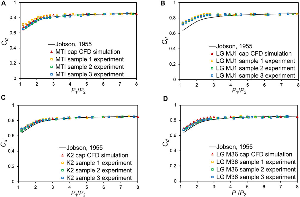
FIGURE 5. RANS simulated discharge coefficients for the MTI cap (A), LG MJ1 cap (B), K2 cap (C), and LG M36 cap (D).

The equivalent areas obtained from CFD simulations were compared with those obtained from experiments. For the MTI cap, the equivalent area obtained through simulations was A_eq = 8.06 mm² while the experimentally-identified area at 95% confidence was A_eq = 8.14 ± 0.337 mm² (Li et al., 2020a). For the LG MJ1 cap, the equivalent area obtained through simulations was A_eq = 8.99 mm² while the experimentally-identified area at 95% confidence was A_eq = 8.62 ± 0.941 mm² (Li et al., 2020a). For the K2 cap, the equivalent area obtained through simulations was A_eq = 7.90 mm² while the experimentally-identified area at 95% confidence was A_eq = 8.50 ± 0.304 mm² (Li et al., 2020a). For the LG M36 cap, the equivalent area obtained through simulations was A_eq = 13.7 mm² while the experimentally-identified area at 95% confidence was A_eq = 11.28 ± 0.196 mm². Discrepancy between the measured and simulated equivalent areas may be caused by variation in the position and shape of the deformed burst disk.

The equivalent areas from, both CFD simulations and experiments showed that the LG M36 cap had the least restriction since its equivalent area was significantly larger than the other three caps. This larger equivalent area is attributed to the large openings that can allow the burst disk to deflect upwards to a greater extent than the other cap designs, resulting in a larger effective area. The MTI, K2, and LG MJ1 all had similar equivalent areas which is attributed to similar size vent holes in the cap.

3.2.3 Ensemble-Averaged Flow Field Analysis

RANS simulations provide the ensemble-averaged flow field which is equivalent to the time-averaged flow field when the process is stationary (i.e. boundary conditions are not changing). The jet Reynolds number was calculated as:

$Re=\frac{\rho UD}{\mu }(11)$

where ρ is air density, μ is molecular viscosity, D is the hydraulic diameter of each individual hole/opening in the positive terminal, and U is the average velocity through each opening. Note that temperature at the jet exit was calculated from isentropic relations and then used in calculating density and molecular viscosity. The average velocity through each opening was calculated using:

$U=\frac{\dot{m}}{NA\rho }(12)$

where $\dot{m}$ is the total mass flow rate through the vent cap, N is the number of openings in the positive terminal, and A is the flow area of a single opening. For a pressure ratio of P₁/P₂ = 7, the resulting Reynolds numbers for the MTI, LG MJ1, K2, and LG M36 caps were 1.06E5, 1.12E5, 7.75E4, and 1.27E5, respectively. The large Reynolds numbers indicate fully turbulent jet flow for each cap (Lee and Chu, 2003).

Contours of velocity magnitude, represented as Mach number, on two orthogonal cross-section planes for each cap are shown in Figure 6 for a pressure ratio of P₁/P₂ = 7. Mach number was calculated as:

$Ma=\frac{U}{c}(13)$

FIGURE 6

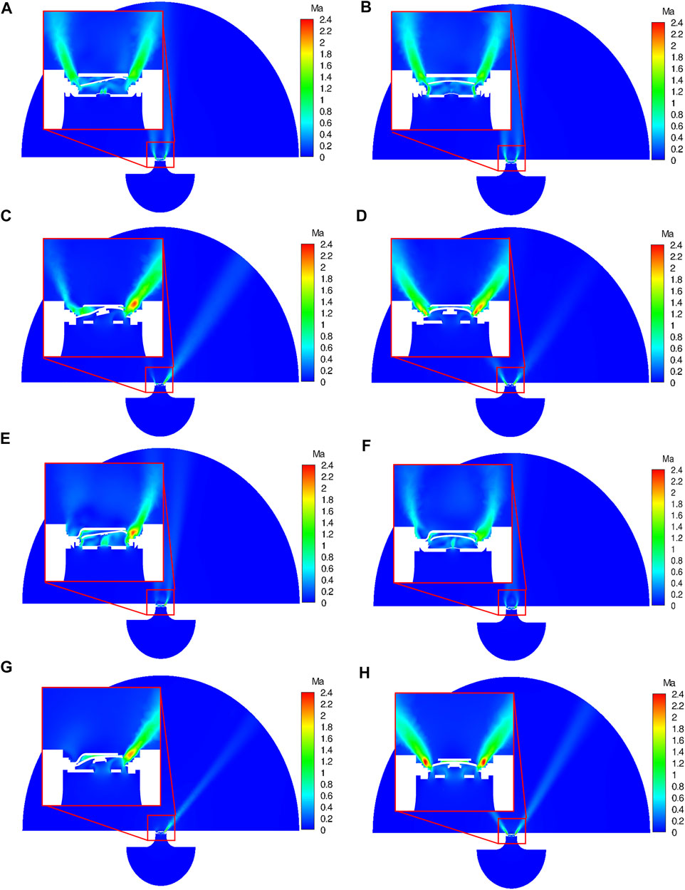
FIGURE 6. RANS simulated Mach number distribution at P₁/P₂ = 7, in the x-normal (left) and z-normal (right) cross-sectional planes for each LIB cap: MTI (A) and (B), LG MJ1 (C) and (D), K2 (E) and (F), and LG M36 (G) and (H).

In Eq. 13, U is the instantaneous velocity magnitude and c is the speed of sound. The speed of sound for an ideal gas is:

$c=\sqrt{\gamma RT} (14)$

where γ is the specific heat capacity ratio, R is the specific gas constant, and T is temperature.

Figure 6A, B show the Mach number contours for the MTI cap in the x-normal and z-normal views, respectively. The maximum Mach number observed in the planes shown in Figures 6A,B was 1.52 while the global maximum Mach number was 1.95. The trajectory of the jets emerging from the MTI cap are shown in the insets of Figures 6A,B. The jets emerge at an angle of approximately 65° relative to the horizontal plane. Figures 6C,D show the Mach number contours for the LG MJ1 cap in the x-normal and z-normal views, respectively. The maximum Mach number observed in the planes shown in Figures 6C,D was 2.30 while the global maximum Mach number was 2.98. The jet trajectory was approximately 50° relative to the horizontal plane. Figures 6E,F show the Mach number contours for the K2 cap in the x-normal and z-normal views, respectively. The maximum Mach number observed in the planes shown in Figures 6E,F was 2.29 while the global maximum Mach number was 2.57. The jet trajectory was approximately 65° relative to the horizontal plane. Finally, Figures 6G,H show the Mach number contours for the LG M36 cap in the x-normal and z-normal views, respectively. The maximum Mach number observed in the planes shown in Figures 6E,F was 2.53 while the global maximum Mach number was 3.04 and the jet trajectory was approximately 50° relative to the horizontal plane. These results and those of section 3.2.2 indicate that the global maximum velocity magnitude through the cap assembly increases with increasing sharp-edge orifice equivalent area.

Figure 7 shows a representation of the jet trajectories emerging from each cap for a pressure ratio of P₁/P₂ = 7 by Mach number isosurfaces of Ma = 0.1 and Ma = 0.3. The jets emerging from the MTI cap, Figure 7A, and K2 cap, Figure 7C, were relatively symmetric compared to the jets emerging from the LG MJ1, Figure 7B, and LG M36 cap, Figure 7D. The jet emerging in the negative z-direction of the LG MJ1 cap in Figure 7B was partially blocked by the presence of the burst disk. No jet emerged in the negative z-direction for the LG M36 in Figure 7D due to asymmetry of the three vent slots in the positive terminal. Thus, the flow of gases through the safety vents may be asymmetrical depending on multiple aspects of the cap design, including the burst disk and positive terminal.

FIGURE 7

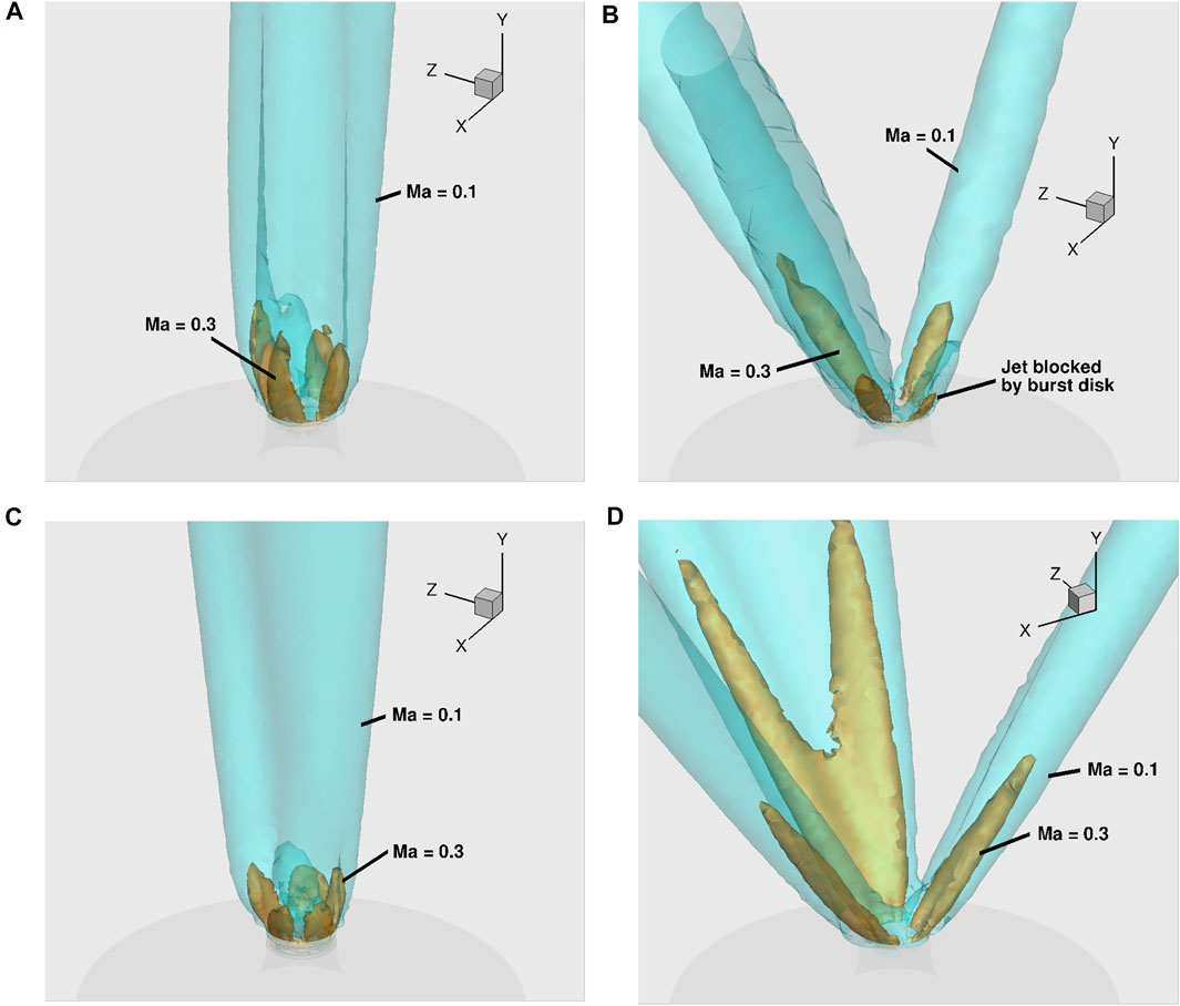
FIGURE 7. RANS simulated Mach number isosurfaces at P₁/P₂ = 7: MTI (A), LG MJ1 (B), K2 (C), and LG M36 (D).

The Mach number distribution in the x-normal viewing plane for the P₁/P₂ = 7 pressure ratio was analyzed further by inserting a streamline which traces the flow originating at the inlet boundary and passes through the hole on the right side of the cap and then exits the domain at the outlet boundary. The streamlines are shown in Figures 8A,D,G,J. The streamlines in Figure 8 were generated as in-plane streamlines, which do not include the normal velocity component. Along each streamline, the Mach number and absolute pressure were extracted and plotted against the y-coordinate. The curves of Mach number plotted against y/D (where D is the diameter of the cell) are shown in Figures 8B,E,H,K for the MTI, LG MJ1, K2, and LG M36 cap, respectively. The curves of absolute pressure plotted against y/D are shown in Figures 8C,F,I,L for the MTI, LG MJ1, K2, and LG M36 cap, respectively.

FIGURE 8

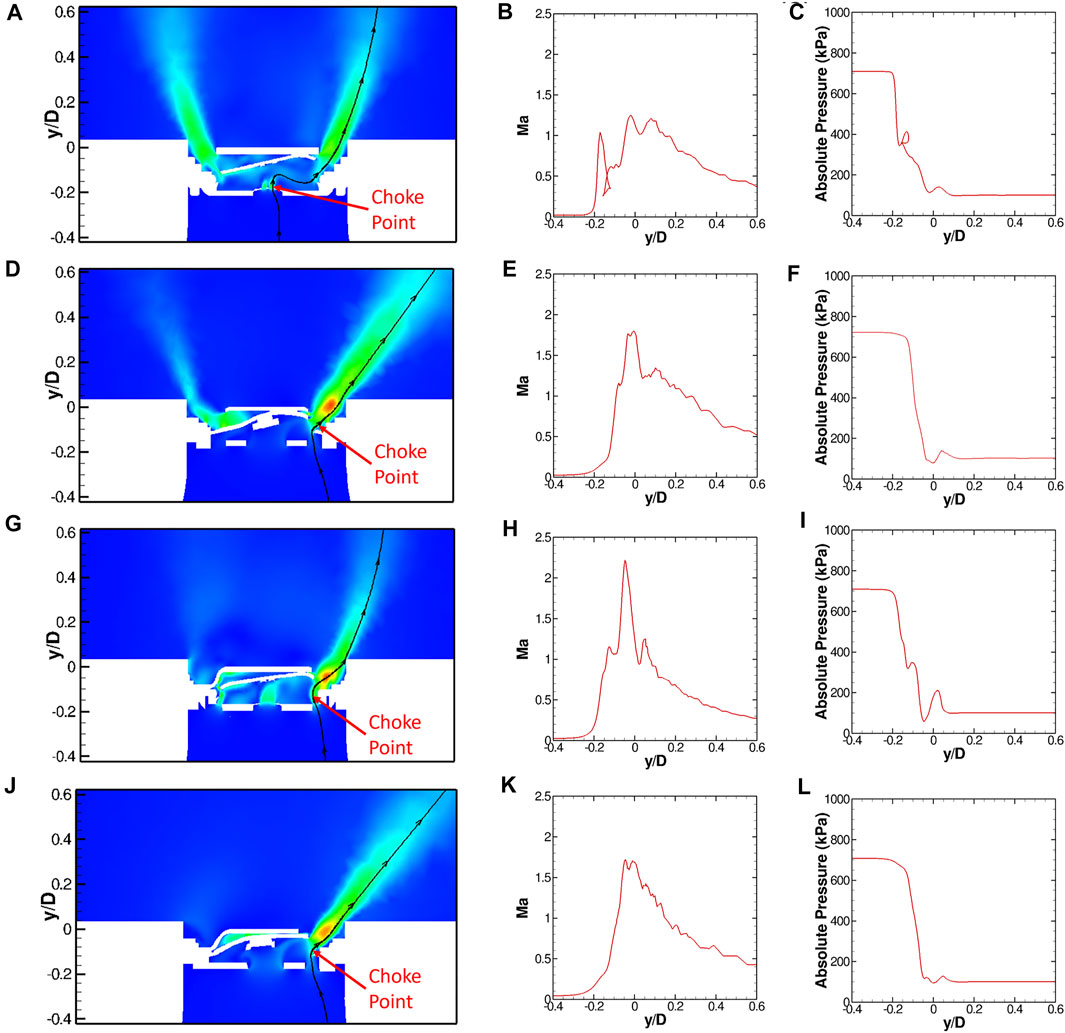
FIGURE 8. RANS simulated Mach number distribution at P₁/P₂ = 7 with a streamline passing through the right vent hole, along with Mach number and absolute pressure extracted along the streamline for: MTI (A, B, and C), LG MJ1 (D, E, and F), K2 (G, H, and I), and LG M36 (J, K, and L) caps.

The streamlines and the data extracted along the streamlines help identify where the flow is accelerated to sonic flow velocity, Ma = 1. For a system having multiple restrictions, the flow may be accelerated to Ma = 1 at more than one location. For the LIB caps, the current collector and the positive terminal plate are considered as two restrictions. For both the MTI and K2 caps, the flow reaches Ma = 1 near the current collector, around y/D = −0.2, as shown in Figures 8A,G. The flow decelerates in the space between the current collector and positive terminal, then accelerates to Ma = 1 again near the positive terminal holes, y/D = -0.1. For the LG MJ1 and LG M36 cells the flow reaches Ma = 1 closer to the positive terminal holes, around y/D = −0.1, as shown in Figures 8D,J. The differences in Mach number distribution through the cap assembly are attributed to differences in cross-sectional flow areas of the components in the LIB cap assembly. The current collector plate of the K2 and MTI caps have smaller cross-sectional flow area than the LG MJ1 and LG M36 cap and it is thus demonstrated that, for this type of cap geometry, the flow first reaches Ma = 1 near both the current collector and near the positive terminal instead of only near the positive terminal.

A choke point in compressible flow systems occurs when the pressure ratio across a restriction is large enough to accelerate the flow to Ma = 1. When choked flow occurs, the mass flow rate through the restriction is independent of the pressure downstream of the restriction, as shown in Eq. 2. The acceleration of flow through the vent caps plays an important role on the overall flow restriction of the cap. For example, the MTI and K2 caps both experience choked flow at the current collector and increasing the area of the positive terminal will not affect the flow rate. For example, the K2 cap has five holes in the positive terminal with an opening area of 20.6 mm² while the MTI cap has four holes with an opening area of 18.5 mm² (Li et al., 2020a). Despite the 10.7% difference in flow area at the positive terminal cap, the two caps have only a 3% difference in the experimentally-measured equivalent area (Li et al., 2020a).

The absolute pressure extracted along the streamlines in Figure 8 was consistent with observed choke plane locations for the P₁/P₂ = 7 pressure ratio. For the MTI and K2 caps, a large decrease in pressure was observed across the current collector (around y/D = −0.2) where the flow accelerated to Ma = 1. The reduction in pressure exceeded the critical pressure ratio, which is a condition required for choked flow to occur. For those two caps, the pressure remains nearly constant between y/D = −0.2 to −0.1. For y/D > −0.1, the pressure decreased to the ambient pressure level as the flow expanded out into the surrounding fluid. For the LG MJ1 and LG M36 caps, the pressure decreased monotonically through the cap.

Figure 9 shows the turbulent viscosity ratio, ${\mu }_T/\mu$, distribution on two orthogonal cross-section planes for each cap at a pressure ratio of P₁/P₂ = 7. In-plane streamlines are also overlaid on Figure 9 to illustrate secondary flow patterns. The left column of images in Figure 9 shows the x-normal view and the right column shows the z-normal view.

FIGURE 9

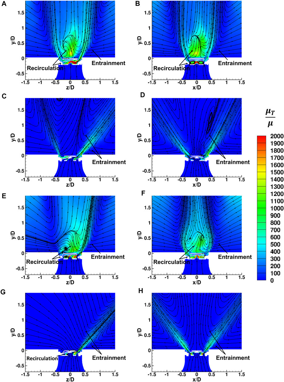
FIGURE 9. RANS simulated turbulent viscosity ratio distribution at P₁/P₂ = 7, in the x-normal (left) and z-normal (right) cross-sectional planes for each LIB cap: MTI (A) and (B), LG MJ1 (C) and (D), K2 (E) and (F), and LG M36 (G) and (H).

For the k-ε family of turbulence models (ANSYS, 2019a), turbulent viscosity is calculated as:

${\mu }_T=\rho C_{\mu }\frac{k^2}{\epsilon }(15)$

where ρ is the fluid density, C_μ is a model constant, k is turbulent kinetic energy, and ε is the turbulent dissipation rate. Turbulent viscosity is added to the molecular viscosity that appears in the momentum transport equations, effectively increasing the transport of momentum due to the presence of turbulence (ANSYS, 2019a). The turbulent viscosity ratio distribution for the MTI cap, Figures 9A,B, shows a large degree of turbulent mixing in three regions: between the current collector and the positive terminal cap, along the jets, and in the region between the jets directly above the vent cap assembly. Turbulence is generated between the current collector and positive terminal cap by two mechanisms: from wall shear as flow passes through the current collector and from flow recirculation (as indicated in the figure). Turbulence is generated along the jets from the shear force generated between the high momentum flow emerging from the vent holes and the low momentum surrounding fluid. Additionally, the steep angle of the jets emerging from the MTI cap causes a recirculation region to form directly above the vent cap, leading to increased turbulent mixing. Surrounding fluid is also entrained in the jets, as indicated in Figures 9A,B.

The turbulent viscosity distribution for the LG MJ1 cap, Figures 9C,D, shows a large degree of turbulent mixing in two regions: between the current collector and positive terminal and along the jets. Streamlines in Figures 9C,D show the shallow angle of the jets emerging from the LG MJ1 cap. There was no recirculation zone above the cap and no significant turbulent mixing in that region. Additionally, the current collector of the LG MJ1 was less restrictive (simulated A_eq = 8.99 mm²) than the MTI current collector (A_eq = 8.06 mm²). The MTI cap has six small holes around the periphery and small holes in the middle of the current collector from spot-weld tearing during CID-activation (Li et al., 2020a). On the other hand, the LG MJ1 current collector has three large slots around the periphery and one large opening in the middle of the current collector from CID-activation (Li et al., 2020a). The geometry of the LG MJ1 cap results in less turbulent mixing from shear and recirculation between the current collector and positive terminal. Generally, turbulent viscosity ratio was lower for the LG MJ1 cap relative to the MTI cap. The LG MJ1 cap showed a global maximum of ${\mu }_T/\mu$ = 3,360 and the MTI cap showed a global maximum of ${\mu }_T/\mu$ = 4,757.

The turbulent viscosity ratio distribution for the K2 cap shown Figures 9E,F was similar to that of the MTI cap which is attributed to the similar geometry of the two caps. The global maximum turbulent viscosity ratio for the K2 cap was ${\mu }_T/\mu$ = 3,855. Likewise, the turbulent viscosity ratio distribution for the LG M36 cap, Figures 9G,H, was similar to that of the LG MJ1 cap due to similar vent cap geometry. The global maximum turbulent viscosity ratio for the LG M36 cap was ${\mu }_T/\mu$ = 2,993. Overall the results show that different cell cap geometries have different degrees and spatial distributions of turbulent mixing with gases flowing through them. These flow aspects will influence combustion of vented flammable gases in a simulation of thermal runaway event (Turns, 2011), and thus can have a significant impact on the predicted heat transfer to the cell’s surroundings.

3.3 Scale-Resolved Simulations of Flow Through LG MJ1 Cap

Scale-resolved simulations (SRS) were conducted on the LG MJ1 cap to analyze the unsteady flow field and dynamic evolution of turbulent structures. The SRS approach is, generally, more expensive but more accurate than RANS turbulence models. One reason that SRS provide improved accuracy is because large scale turbulent eddies, which account for most of the turbulent transport, tend to be anisotropic (ANSYS, 2019a). The anisotropy may be captured in certain RANS models, such as the Reynolds-Stress model, but this model requires additional transport equations and is more computationally expensive than the one- or two-equation models (ANSYS, 2019a). The one- and two-equation RANS models consider the turbulence to be isotropic and provide a good balance of computation speed and accuracy (ANSYS, 2019a).

SRS capture the spectrum of turbulent scales to varying degrees, depending on the model. Direct numerical simulation (DNS) is the most expensive but most accurate method. There is no turbulence modeling in DNS and even the smallest eddies are resolved. DNS is typically reserved for simplified cases and lower Reynolds number flows. Large edge simulation (LES) captures the larger scales but models the smaller scales, operating under the assumption that the smaller scales are more isotropic and more easily modeled (ANSYS, 2019a). Both DNS and LES are computationally expensive, requiring a large number of elements and small time steps. A relatively new class of hybrid RANS-LES turbulence models has been developed, which combines the best features of RANS and LES (ANSYS, 2019a). In regions where the mesh size is fine enough, the LES model is used. In other regions where the mesh size is too coarse for LES, then the RANS model is used.

The SBES hybrid turbulence model was used to simulate flow through LG MJ1 cap to gain additional insight into the flow field beyond what is capable from a purely RANS approach. The SBES model is similar to the detached eddy simulation (DES) model, but uses an improved shielding function to transition between RANS and LES modeled regions (ANSYS, 2019a). However, when using the SBES models, the mesh size has a significant effect on the shielding function which determines the transition between RANS and scale-resolved regions (ANSYS, 2019a). The series of conical refinement regions, described previously in section 2.2, ensured transition from RANS to LES in the region above the vent cap. The final mesh for SRS had 6.33E6 polyhedral elements.

SRS were conducted at a pressure ratio of P₁/P₂ = 23.7, which represents the typical pressure difference across the cap at the moment of venting (Li et al., 2020b). This differs from the RANS simulations which were conducted at lower pressure ratios, 1.2 ≤ P₁/P₂ ≤ 8, to maintain consistency with the pressure ratios used in the independent experiments for LIB cap discharge coefficients (Li et al., 2020a).

To ensure that the SRS solution was statistically-stationary, the simulation was carried out for 4 ms. The solution was monitored to ensure that mean field variables were independent of time. Between 4 and 7 ms, flow field statistics were recorded to analyze mean and RMS quantities. Figure 10 shows the SRS results. Figure 10A shows an x-normal view and Figure 10B shows a z-normal view of instantaneous velocity magnitude contours taken at a flow time of 7 ms. Note that the Mach disk is visible at the right jet in Figure 10A, and to a lesser extent in Figure 10B. The instantaneous velocity contours show the highly turbulent flow field, as evidenced by the break-up of the jet and mixing of the high momentum jet with the quiescent surrounding air.

FIGURE 10

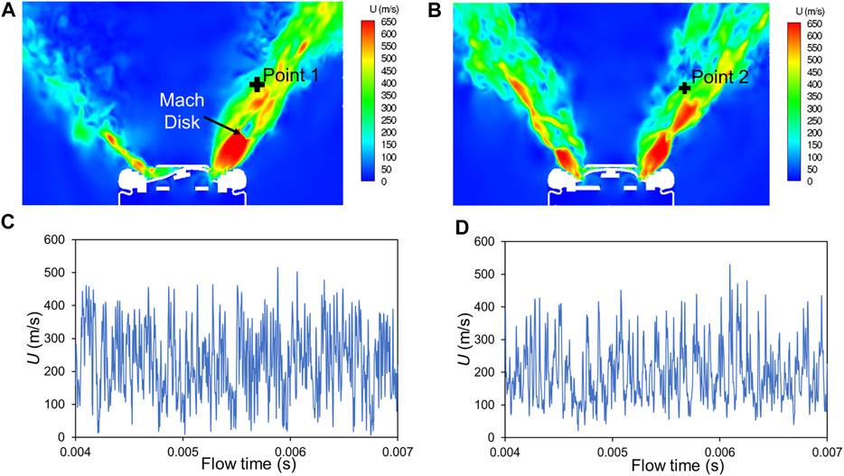
FIGURE 10. SRS simulated instantaneous velocity magnitude for the LG MJ1 cap at P₁/P₂ = 23.7 in the x-normal (A) and z-normal (B) planes and instantaneous velocity magnitude plotted for 3 ms of flow time for point 1 (C) and point 2 (D).

The instantaneous velocity magnitude at two points in the jet flow emerging from the holes of the cap were monitored to illustrate the magnitude and frequency of the turbulence in the jet. Point 1 was located at the inner edge of the right jet in the x-normal plane. Point 2 was located at the inner edge of the right jet in the z-normal plane. The instantaneous velocity magnitude at these two points was plotted over the course of 3 ms of flow time in Figures 10C,D, respectively. The mean velocity magnitudes at point 1 and 2 were 230.66 and 196.41 m/s, respectively. The root mean square (RMS) velocity magnitudes at point 1 and 2 were 102.75 and 86.96 m/s, respectively. Turbulence intensity, which is equal to RMS velocity divided by mean velocity, was 50.4 and 44.3% at points 1 and 2, respectively. The observed turbulence intensity of ∼50% indicates highly turbulent flow (ANSYS, 2019b).

The contours of the mean velocity magnitude, represented by Mach number, are shown for the x-normal and z-normal planes in Figures 11A,B, respectively. In the x-normal cross-sectional plane, the effects of the presence of the deformed burst disk was observed as previously in the RANS simulations. The burst disk remained attached and resulted in asymmetric jet structure for the left and right jets in Figure 11A. The maximum velocity in Figure 11A reached Ma = 4.03 immediately downstream of the right vent hole. The global maximum velocity was Ma = 4.18. The two vent holes shown in the z-normal plane were more symmetric, as shown in Figure 11B.

FIGURE 11

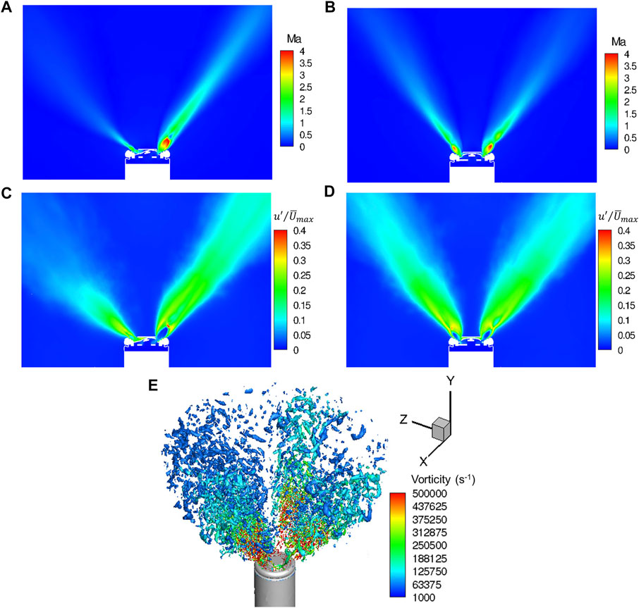
FIGURE 11. SRS simulated mean velocity, represented by Mach number, at P₁/P₂ = 23.7 for the LG MJ1 cap in the x-normal (A) and z-normal (B) planes, normalized fluctuating velocity magnitude in the x-normal (C) and z-normal planes (D), and a 3-D isosurface taken at normalized Q-criterion = 0.3 colored by vorticity magnitude which illustrates coherent turbulence structures in the jet flow (E).

Contours of normalized RMS velocity ($u^{\prime }/{\overline{U}}_{max}$) in the x-normal and z-normal planes are shown in Figures 11C,D. The highest level of fluctuating velocity observed was in the right jet of the x-normal plane. The value of normalized RMS velocity of the right jet was $u^{\prime }/{\overline{U}}_{max}$ = 0.41. Due to the blockage from the burst disk, the maximum fluctuating velocity of the left jet was $u^{\prime }/{\overline{U}}_{max}$ = 0.29. The global maximum was $u^{\prime }/{\overline{U}}_{max}$ = 0.48. In general, higher levels of fluctuating velocity were observed at the edges of the jet, corresponding to the position of the shear layer between the jet and the quiescent fluid. The shear created between the high momentum and low momentum fluid creates unsteadiness and enhances the mixing between the two fluids.

Isosurfaces of a normalized Q-criterion from the SRS simulation was used to visualize the turbulence developing in the jet region. The normalized Q-criterion is derived based on the second invariant of the velocity gradient tensor and is useful for identifying coherent turbulent structures (ANSYS, 2019a). Figure 11E shows an instantaneous 3-D isosurface taken at a constant normalized Q-criterion value of 0.3. The coherent structures developing near the battery cap grew in size as they lost momentum and travelled downstream. The isosurface is colored by vorticity magnitude, which illustrates the strength of rotation of the coherent structures. The smaller structures near the cap had high vorticity and the vorticity decreased as the structures traveled downstream. A video showing the evolution of the normalized Q-criterion isosurfaces is shown in Supplementary Video S1.

The SRS simulation results, conducted at a pressure ratio of P₁/P₂ = 23.7, showed the structure of the high velocity and highly turbulent jets emerging from the vent holes. The large pressure ratio accelerated the flow to a global maximum velocity magnitude of Ma = 4.18. Unsteadiness introduced by the shear between the high momentum jet and low momentum surrounding fluid resulted in a high value of normalized fluctuating velocity, up to $u^{\prime }/{\overline{U}}_{max}$ = 0.48. The 3-D isosurfaces taken at normalized Q-criterion = 0.3 further illustrate the highly turbulent flow by the large number of coherent vortex structures in the jet. The coherent structures grow larger in scale while vorticity decreases as the vortices travel downstream in the jet.

4 Conclusion

In the present work, a RANS CFD model was developed to simulate the steady state venting flow emerging from four LIB caps. The sharp-edge orifice equivalent area for each battery cap obtained from CFD was compared with experiments. The simulated equivalent area agreed well for the MTI, LG MJ1, and K2 caps but under-predicted equivalent area for the LG M36 which was attributed to possible variation in the burst disk position and shape. The steady state velocity field of the flow through the LIB cap obtained from the CFD model showed that at higher pressure ratios, choked flow occurred at varying points for each of the four caps. For the MTI and K2 caps, the choke point occurred near the current collector of the cap which was attributed to low cross-sectional flow area through that component. For the LG MJ1 and LG M36 caps, the choke point was closer to the holes in the positive terminal plate. The choke point location plays an important role in the design of the safety vent since an overly restrictive current collector plate will minimize the benefit from having a positive terminal plate with large flow area. Turbulent viscosity ratio distributions for all four vent caps showed increased turbulent mixing in two regions: between the current collector and positive terminal and along the jets. For the MTI and K2 caps, the steep jet angle caused flow recirculation directly above the vent cap which led to a third region of increased turbulent mixing. The global maximum turbulent viscosity ratio (${\mu }_T/\mu$) of the MTI, LG MJ1, K2, and LG M36 caps at pressure ratio of P₁/P₂ = 7 were 4,575, 3,360, 3,855, and 2,993, respectively. Increased turbulent mixing may play an important role in combustion of vented gases (Turns, 2011).

To investigate the turbulent flow field in more detail, scale-resolved simulations (SRS) using the SBES turbulence model were implemented using the LG MJ1 cap. The mean and fluctuating velocity distributions showed that the shear between the high velocity jets and the surrounding quiescent fluid resulted in high levels of fluctuating velocity and, thus, high levels of turbulence intensity. The high levels of fluctuating velocity in the jets agreed with high levels of turbulent viscosity in the jets predicted by RANS simulations. The deformation geometry of the burst disk partially blocked one of the four holes of the positive terminal. The velocity magnitude and the RMS velocity fluctuations for the jet from this partially blocked hole were both dampened. The size and rotation of coherent turbulent structures were also visualized from the SBES simulation results. The coherent structures grew in size as they lost momentum and travelled downstream and the vorticity of those structures also decreased as they traveled downstream. The turbulence intensity and length scale both play an important role in battery safety as both parameters will influence the magnitude of impingement heat transfer from the jets to neighboring surfaces or cells (Kataoka et al., 1987). Thus, the complex turbulence structure of jets emerging from an 18650 Li-ion battery cap, as demonstrated by these SBES simulations, can have a significant impact on model simulations of heat transfer from a Li-ion cell undergoing thermal runaway.

The present work provides a foundation for using highly detailed, 3-D CFD modeling to simulate the venting flow in commercial LIB cells. In the future work, the CFD model will be used to investigate the influence of the flow field on heat transfer to neighboring surfaces. Ultimately, this modeling approach can help improve the design of battery modules to protect against propagating failures driven by venting, combustion, and fire.

Data Availability Statement

The raw data supporting the conclusions of this article will be made available by the authors, without undue reservation.

Author Contributions

All authors listed have made a substantial, direct and intellectual contribution to the work, and approved it for publication. WL contributed to CFD model development, conducted simulations, performed data reduction, analyzed the results, and prepared the manuscript. VQ contributed to the CFD model development and conducted simulations. KC prepared the LIB cap samples, edited the manuscript, and was responsible for project management. JO analyzed the results, edited the manuscript, and was responsible for funding acquisition and project management.

Conflict of Interest

The authors declare that the research was conducted in the absence of any commercial or financial relationships that could be construed as a potential conflict of interest.

Publisher’s Note

All claims expressed in this article are solely those of the authors and do not necessarily represent those of their affiliated organizations, or those of the publisher, the editors and the reviewers. Any product that may be evaluated in this article, or claim that may be made by its manufacturer, is not guaranteed or endorsed by the publisher.

Acknowledgments

The authors acknowledge financial support from the Naval Surface Warfare Center, Crane Division under the Naval Innovative Science and Engineering Program. We also acknowledge Kyle Stoll from the Naval Surface Warfare Center, Crane Division for his assistance in the CT imaging of the MTI, LG MJ1, K2 and LG M36 cap. WL also acknowledges the Purdue University Andrews Fellowship Program and the Indiana Manufacturing Competitiveness Center (IN-MaC) for financial support on this project. The U.S. Government is authorized to reproduce and distribute reprints for governmental purposes notwithstanding any copy-right notation thereon. The views and conclusions contained herein are those of the authors and should not be interpreted as necessarily representing the official policies or endorsements, either expressed or implied, of the Naval Surface Warfare Center, Crane Division or the U.S. Government.

Supplementary Material

The Supplementary Material for this article can be found online at: https://www.frontiersin.org/articles/10.3389/fenrg.2021.788239/full#supplementary-material

References

Abada, S., Petit, M., Lecocq, A., Marlair, G., Sauvant-Moynot, V., and Huet, F. (2018). Combined Experimental and Modeling Approaches of the thermal Runaway of Fresh and Aged Lithium-Ion Batteries. J. Power Sourc. 399, 264–273. doi:10.1016/j.jpowsour.2018.07.094

CrossRef Full Text | Google Scholar

Adamson, T. C., and Nicholls, J. A. (1959). On the Structure of Jets from Highly Underexpanded Nozzles into Still Air. J. Aerospace Sci. 26 (1), 16–24. doi:10.2514/8.7912

CrossRef Full Text | Google Scholar

ANSYS (2019a). ANSYS FLUENT 19.2 Theory Guide. Canonsburg, PA: ANSYS Inc.

Google Scholar

ANSYS (2019b). ANSYS FLUENT 19.2 User’s Guide. Canonsburg, PA: ANSYS Inc.

Google Scholar

ANSYS (2019c). ANSYS Meshing User's Guide. Canonsburg, PA: ANSYS Inc.

Google Scholar

Archibald, E., Kennedy, R., Marr, K., Jeevarajan, J., and Ezekoye, O. (2020). Characterization of Thermally Induced Runaway in Pouch Cells for Propagation. Fire Technol. 56, 2467–2490. doi:10.1007/s10694-020-00974-2

CrossRef Full Text | Google Scholar

Bugryniec, P. J., Davidson, J. N., and Brown, S. F. (2020). Computational Modelling of thermal Runaway Propagation Potential in Lithium Iron Phosphate Battery Packs. Energ. Rep. 6, 189–197. doi:10.1016/j.egyr.2020.03.024

CrossRef Full Text | Google Scholar

Chen, D., Jiang, J., Kim, G.-H., Yang, C., and Pesaran, A. (2016). Comparison of Different Cooling Methods for Lithium Ion Battery Cells. Appl. Therm. Eng. 94, 846–854. doi:10.1016/j.applthermaleng.2015.10.015

CrossRef Full Text | Google Scholar

Cheng, X., Li, T., Ruan, X., and Wang, Z. (2019). Thermal Runaway Characteristics of a Large Format Lithium-Ion Battery Module. Energies 12 (16), 3099. doi:10.3390/en12163099

CrossRef Full Text | Google Scholar

Coman, P. T., Rayman, S., and White, R. E. (2016). A Lumped Model of Venting during thermal Runaway in a Cylindrical Lithium Cobalt Oxide Lithium-Ion Cell. J. Power Sourc. 307, 56–62. doi:10.1016/j.jpowsour.2015.12.088

CrossRef Full Text | Google Scholar

Coman, P. T., Mátéfi-Tempfli, S., Veje, C. T., and White, R. E. (2017). Modeling Vaporization, Gas Generation and Venting in Li-Ion Battery Cells with a Dimethyl Carbonate Electrolyte. J. Electrochem. Soc. 164 (9), A1858–A1865. doi:10.1149/2.0631709jes

CrossRef Full Text | Google Scholar

Dong, T., Peng, P., and Jiang, F. (2018). Numerical Modeling and Analysis of the thermal Behavior of NCM Lithium-Ion Batteries Subjected to Very High C-Rate Discharge/charge Operations. Int. J. Heat Mass Transfer 117, 261–272. doi:10.1016/j.ijheatmasstransfer.2017.10.024

CrossRef Full Text | Google Scholar

Feng, X., Ouyang, M., Liu, X., Lu, L., Xia, Y., and He, X. (2018). Thermal Runaway Mechanism of Lithium Ion Battery for Electric Vehicles: A Review. Energ. Storage Mater. 10, 246–267. doi:10.1016/j.ensm.2017.05.013

CrossRef Full Text | Google Scholar

Hatchard, T. D., MacNeil, D. D., Basu, A., and Dahn, J. R. (2001). Thermal Model of Cylindrical and Prismatic Lithium-Ion Cells. J. Electrochem. Soc. 148 (7), A755–A761. doi:10.1149/1.1377592

CrossRef Full Text | Google Scholar

Jobson, D. A. (1955). On the Flow of a Compressible Fluid through Orifices. Proc. Inst. Mech. Eng. 169 (1), 767–776. doi:10.1243/PIME_PROC_1955_169_077_02

CrossRef Full Text | Google Scholar

Jothi, T. J. S., and Srinivasan, K. (2019). Shock Structures of Underexpanded Non-circular Slot Jets. Sādhanā 44 (1), 25. doi:10.1007/s12046-018-0988-6

CrossRef Full Text | Google Scholar

Kataoka, K., Suguro, M., Degawa, H., Maruo, K., and Mihata, I. (1987). The Effect of Surface Renewal Due to Largescale Eddies on Jet Impingement Heat Transfer. Int. J. Heat Mass Transfer 30 (3), 559–567. doi:10.1016/0017-9310(87)90270-5

CrossRef Full Text | Google Scholar

Kayser, J. C., and Shambaugh, R. L. (1991). Discharge Coefficients for Compressible Flow through Small-Diameter Orifices and Convergent Nozzles. Chem. Eng. Sci. 46 (7), 1697–1711. doi:10.1016/0009-2509(91)87017-7

CrossRef Full Text | Google Scholar

Kim, G.-H., Pesaran, A., and Spotnitz, R. (2007). A Three-Dimensional thermal Abuse Model for Lithium-Ion Cells. J. Power Sourc. 170 (2), 476–489. doi:10.1016/j.jpowsour.2007.04.018

CrossRef Full Text | Google Scholar

Larsson, F., Bertilsson, S., Furlani, M., Albinsson, I., and Mellander, B.-E. (2018). Gas Explosions and thermal Runaways during External Heating Abuse of Commercial Lithium-Ion Graphite-LiCoO2 Cells at Different Levels of Ageing. J. Power Sourc. 373, 220–231. doi:10.1016/j.jpowsour.2017.10.085

CrossRef Full Text | Google Scholar

Lee, J. H. W., and Chu, V. H. (2003). “Turbulent Jets,” in Turbulent Jets and Plumes (Boston, MA: Springer). doi:10.1007/978-1-4615-0407-8_2

CrossRef Full Text | Google Scholar

Li, W., Crompton, K. R., Hacker, C., and Ostanek, J. (2020a). “Analysis of Lithium-Ion Battery Cap Structure and Characterization of Venting Parameters,” in ASME 2020 International Mechanical Engineering Congress and Exposition (ASME). V008T08A020.

CrossRef Full Text | Google Scholar

Li, W., Crompton, K. R., Hacker, C., and Ostanek, J. K. (2020b). Comparison of Current Interrupt Device and Vent Design for 18650 Format Lithium-Ion Battery Caps. J. Energ. Storage 32, 101890. doi:10.1016/j.est.2020.101890

CrossRef Full Text | Google Scholar

Lopez, C. F., Jeevarajan, J. A., and Mukherjee, P. P. (2016). Evaluation of Combined Active and Passive Thermal Management Strategies for Lithium-Ion Batteries. J. Electrochem. Energ. Convers. Storage 13, 031007. doi:10.1115/1.4035245

CrossRef Full Text | Google Scholar

Mao, B., Zhao, C., Chen, H., Wang, Q., and Sun, J. (2021). Experimental and Modeling Analysis of Jet Flow and Fire Dynamics of 18650-type Lithium-Ion Battery. Appl. Energ. 281, 116054. doi:10.1016/j.apenergy.2020.116054

CrossRef Full Text | Google Scholar

Mishra, D., Shah, K., and Jain, A. (2021). Investigation of the Impact of Flow of Vented Gas on Propagation of Thermal Runaway in a Li-Ion Battery Pack. J. Electrochem. Soc. 168 (6), 060555. doi:10.1149/1945-7111/ac0a20

CrossRef Full Text | Google Scholar

Nedjalkov, A., Meyer, J., Köhring, M., Doering, A., Angelmahr, M., Dahle, S., et al. (2016). Toxic Gas Emissions from Damaged Lithium Ion Batteries-Analysis and Safety Enhancement Solution. Batteries 2 (1), 5. doi:10.3390/batteries2010005

CrossRef Full Text | Google Scholar

Norum, T. D., and Seiner, J. M. (1982). Broadband Shock Noise from Supersonic Jets. AIAA J. 20 (1), 68–73. doi:10.2514/3.51048

CrossRef Full Text | Google Scholar

Ostanek, J. K., Li, W., Mukherjee, P. P., Crompton, K. R., and Hacker, C. (2020). Simulating Onset and Evolution of thermal Runaway in Li-Ion Cells Using a Coupled thermal and Venting Model. Appl. Energ. 268, 114972. doi:10.1016/j.apenergy.2020.114972

CrossRef Full Text | Google Scholar

Parhizi, M., Crompton, K. R., and Ostanek, J. K. (2021). “Probing the Role of Venting and Evaporative Cooling on Thermal Runaway for Small Format Li-Ion Cells,” in ASME International Mechanical Engineering Congress and Exposition (ASME). (Virtual/Online).

Google Scholar

Peng, P., and Jiang, F. (2016). Thermal Safety of Lithium-Ion Batteries with Various Cathode Materials: A Numerical Study. Int. J. Heat Mass Transfer 103, 1008–1016. doi:10.1016/j.ijheatmasstransfer.2016.07.088

CrossRef Full Text | Google Scholar

Perry, J. A. (1949). Critical Flow through Sharp-Edged Orifices. Trans. Am. Soc. Mech. Eng. 71, 757–765.

Google Scholar

Prada, E., Di Domenico, D., Creff, Y., Bernard, J., Sauvant-Moynot, V., and Huet, F. (2012). Simplified Electrochemical and Thermal Model of LiFePO4-Graphite Li-Ion Batteries for Fast Charge Applications. J. Electrochem. Soc. 159 (9), A1508–A1519. doi:10.1149/2.064209jes

CrossRef Full Text | Google Scholar

Ren, D., Liu, X., Feng, X., Lu, L., Ouyang, M., Li, J., et al. (2018). Model-based thermal Runaway Prediction of Lithium-Ion Batteries from Kinetics Analysis of Cell Components. Appl. Energ. 228, 633–644. doi:10.1016/j.apenergy.2018.06.126

CrossRef Full Text | Google Scholar

Stoll, K. D., Crompton, K. R., Hacker, C. D., Li, W., and Ostanek, J. K. (2020a). LG MJ1 Vent Cap CT Scans. West Lafayette, IN: Purdue University Research Repository. doi:10.4231/YA7S-H420

CrossRef Full Text | Google Scholar

Stoll, K. D., Crompton, K. R., Hacker, C. D., Li, W., and Ostanek, J. K. (2020b). MTI 18650 Vent Cap CT Scans. West Lafayette, IN: Purdue University Research Repository. doi:10.4231/61G4-S939

CrossRef Full Text | Google Scholar

Stoll, K. D., Crompton, K. R., Hacker, C. D., Li, W., and Ostanek, J. K. (2021a). K2 18650 Vent Cap CT Scans. West Lafayette, IN: Purdue University Research Repository. doi:10.4231/5KKV-1998

CrossRef Full Text | Google Scholar

Stoll, K. D., Crompton, K. R., Hacker, C. D., Li, W., and Ostanek, J. K. (2021b). LG M36 Vent Cap CT Scans. West Lafayette, IN: Purdue University Research Repository. doi:10.4231/WCFR-9M25

CrossRef Full Text | Google Scholar

Turns, S. R. (2011). “Turbulent Nonpremixed Flames,” in An Introduction to Combustion: Concepts and Applications. third ed. (New York, NY: McGraw-Hill).

Google Scholar

Walker, W. Q., Darst, J. J., Finegan, D. P., Bayles, G. A., Johnson, K. L., Darcy, E. C., et al. (2019). Decoupling of Heat Generated from Ejected and Non-ejected Contents of 18650-format Lithium-Ion Cells Using Statistical Methods. J. Power Sourc. 415, 207–218. doi:10.1016/j.jpowsour.2018.10.099

CrossRef Full Text | Google Scholar

Wang, Q., Ping, P., Zhao, X., Chu, G., Sun, J., and Chen, C. (2012). Thermal Runaway Caused Fire and Explosion of Lithium Ion Battery. J. Power Sourc. 208, 210–224. doi:10.1016/j.jpowsour.2012.02.038

CrossRef Full Text | Google Scholar

Wang, Q., Mao, B., Stoliarov, S. I., and Sun, J. (2019). A Review of Lithium Ion Battery Failure Mechanisms and Fire Prevention Strategies. Prog. Energ. Combustion Sci. 73, 95–131. doi:10.1016/j.pecs.2019.03.002

CrossRef Full Text | Google Scholar

Xu, X. M., Li, R. Z., Zhao, L., Hu, D. H., and Wang, J. (2018). Probing the thermal Runaway Triggering Process within a Lithium-Ion Battery Cell with Local Heating. AIP Adv. 8 (10), 105323. doi:10.1063/1.5039841

CrossRef Full Text | Google Scholar

Zhong, G., Li, H., Wang, C., Xu, K., and Wang, Q. (2018). Experimental Analysis of Thermal Runaway Propagation Risk within 18650 Lithium-Ion Battery Modules. J. Electrochem. Soc. 165 (9), A1925–A1934. doi:10.1149/2.0461809jes

CrossRef Full Text | Google Scholar

Nomenclature

A flow area

A_eq sharp-edge orifice equivalent flow area

c speed of sound

C_d discharge coefficient

C_μ k-ε turbulence model constant

c_p specific heat at constant pressure

c_v specific heat at constant volume

D orifice diameter, or cell diameter

k turbulence kinetic energy

L thickness of the orifice plate

L_s the first shock cell length

Ma Mach number

Re Reynolds number

$\dot{\mathit{m}}$ mass flow rate of air through a restriction

${\dot{\mathit{m}}}_{\mathit{i}\mathit{d}\mathit{e}\mathit{a}\mathit{l}}$ ideal mass flow rate

$\overline{\mathit{p}}$ mean pressure

P₁ upstream total pressure

P₂ downstream total pressure

r radial coordinate

R gas constant for air

$\overline{\mathit{T}}$ mean temperature

T local, instantaneous temperature

T₁ upstream total temperature

${\overline{\mathit{u}}}_{\mathit{i}}$ mean velocity vector

${\mathit{u}}_{\mathit{i}}^{\prime }$ fluctuating velocity vector

u′ local, RMS velocity magnitude

U local, instantaneous velocity magnitude

$\overline{\mathit{U}}$ local, mean velocity magnitude

${\overline{\mathit{U}}}_{max}$ global maximum of mean velocity magnitude

x x-coordinate

y y-coordinate

z z-coordinate

Greek

γ ratio of specific heats

ε turbulence dissipation rate

ρ fluid density

λ thermal conductivity

λ_T turbulent thermal conductivity

μ molecular viscosity

${\mathit{\mu }}_{\mathit{T}}$ turbulent viscosity

List of Abbreviations

CFD Computational Fluid Dynamics

CT Computed Tomography

LIB Lithium-ion Battery

NCM Nickel Cobalt Manganese

RANS Reynolds-Averaged Navier-Stokes

SEI Solid Electrolyte Interphase

SRS Scale-Resolving Simulations