 Yuping Wang
 Weidong Li
- 1School of Transport and Logistics Engineering, Wuhan University of Technology, Wuhan, China
- 2Faculty of Engineering, Environment and Computing, Coventry University, Coventry, United Kingdom
New energy vehicles are crucial for low carbon applications of renewable energy and energy storage, while effective fault diagnostics of their rolling bearings is vital to ensure the vehicle’s safe and effective operations. To achieve satisfactory rolling bearing fault diagnosis of the new energy vehicle, a transfer-based deep neural network (DNN-TL) is proposed in this study by combining the benefits of both deep learning (DL) and transfer learning (TL). Specifically, by first constructing the convolutional neural networks (CNNs) and long short-term memory (LSTM) to preprocess vibration signals of new energy vehicles, the fault-related preliminary features could be extracted efficiently. Then, a grid search method called step heapsort is designed to optimize the hyperparameters of the constructed model. Afterward, both feature-based and model-based TLs are developed for the fault condition classifications transfer. Illustrative results show that the proposed DNN-TL method is able to recognize different faults accurately and robustly. Besides, the training time is significantly reduced to only 18s, while the accuracy is still over 95%. Due to the data-driven nature, the proposed DNN-TL could be applied to diagnose faults of new energy vehicles, further benefitting low carbon energy applications.
Introduction
New energy vehicles such as the electrical vehicle and hybrid electrical vehicle play a vital role in achieving low carbon industrial and energy economy, where the rolling bearing is a key component within new energy vehicles. To ensure the effective operations and satisfactory functions of new energy vehicles, the health state of rolling bearings must be well-kept during new energy vehicle operations. However, due to complex working conditions, faults of the rolling bearing in the inner and outer races, the rolling element or gearwheel, such as pitting, peeling, crack, or indentation, are not rare in practice (Zhao et al., 2019). According to statistics, bearing failures account for 45–55% of equipment destruction (Hoang and Kang, 2019). Therefore, the study of effective fault diagnosis is of great significance to improve the safety and reliability of new energy vehicles, further benefitting a low carbon society.
Recently, based on the artificial intelligence technologies, data-driven fault diagnostics methods have received extensive attention from researchers (Liu et al., 2020; Ren et al., 2020; Li et al., 2021a; Liu et al., 2021a; Li et al., 2021b; Liu et al., 2021b; Hongcan and Wang, 2021). On the one hand, after predefining the features, faults could be classified by conventional machine learning (ML) algorithms. Popularly used conventional ML algorithms include the support vector machine (SVM) (Feng et al., 2020), logistic regression (LR), nearest neighbor algorithm (KNN) (Syaifullah et al., 2021), and random forest (RF). The characteristics of these algorithms are easy training and good computing performance. For traditional ML-based methods, their effectiveness largely depends on features. In order to facilitate the methods, signal processing algorithms have been designed as data preprocessors to support feature acquisition. However, it is time-consuming and labor-intensive and even needs manual efforts by professional technicians.
On the other hand, feature extraction is conducted autonomously by DL algorithms from large-volume data and fault classification (Li et al., 2021c), where artificial neural network (ANN) (Lecun et al., 2015), stacked autoencoder (SAE) (Chine et al., 2016), CNNs (Zhang et al., 2018; Wang et al., 2020a), deep belief network (DBN) (Shujaat et al., 2020), and recurrent neural network (RNN) (Szegedy et al., 2017a; Chen and Pan, 2021) have been widely used for fault diagnostics in new energy vehicles. For example, Jia et al. (2016a) proposed stacked multiple AEs to extract features from raw bearing vibration signals. The average accuracies of both training and testing are 100%. Because of the complexity of the original signal data, the AE method lacks robustness. To overcome the drawback of AE, Shao et al. (2017a) proposed a novel loss for AE by adopting maximum correntropy. The average accuracy of the method is 94.05%. The original AE and its deformation cannot guarantee the usefulness of feature extraction (Shao et al., 2017a). Shao et al. (2017b) proposed an improved depth AE model from combination of DAE and comparative AE (CAE). After feature fusion, the average testing accuracy of the method is 95.19%. Because of applying the CD algorithm, some researchers study RBM widely. Chen et al. (2017) proposed methods for extracting bearing fault features DBM and DBN. The accuracy of classification achieves more than 99%. Shao et al. (2015) proposed PSO to the DBN for fault diagnosis. Janssens et al. (2016) proposed feature learning based on CNNs using two sensors to collect vibration signals. The CNN-based method yields an overall increase in the accuracy of classification around 6 percent, without relying on extensive domain knowledge for detecting faults. Guo et al. (2016) proposed a hierarchical CNNs method with an adaptive learning rate to classify bearing faults. The model achieved a high accuracy and offered an automatic feature extraction procedure which is practical and convenient for use in fault diagnosis. Wang et al. (2020b) proposed multi-head attention and a convolutional neural network. The diagnosis rates of bearing states under working loads of 0–3 hp all reach over 99%. All the above research studies illustrate that DL-based methods can autonomously retrieve features from the monitoring signals of new energy vehicles, which has great flexibility instead of transforming and extracting features manually. In a sense, RNN is the deepest model (Schmidhuber, 2015). RNN can only deal with short-term dependency problems. LSTM is a special RNN that can handle both short-term and long-term dependency problems. Signals from new energy vehicles are time series data in nature, so LSTM is also a promising tool for fault diagnosis. However, some limitations are still required to be solved by using DL methods such as 1) a large amount of data are generally required for the DL training process, especially DL; 2) Most of DL algorithms have various hyperparameters, and the optimization process of these hyperparameters is cumbersome with high computational burden; and 3) Some assumptions must be met such as the source domain and the target domain. When the above conditions are not met, the DL algorithm could not be able to extract effective features outside these assumptions, further resulting in the underfitting or overfitting issues. As the DL-based methods are only suitable for specific conditions (Jia et al., 2016b), it is difficult to meet in practice.
Table 1 illustrates the difference between ML and TL. In general, TL methods could be divided into four categories: instance-based transfer learning (ITL), feature-based transfer learning (FTL), model-based transfer learning (MTL), and relation-based transfer learning (RTL). ITL transfers the samples of the source domain to the target domain through weight reuse. FTL transforms features to find a common latent space. MTL is to build a feature sharing model. Some features are pre-trained in the source domain and transferred to the target domain for use. Neural networks mainly use MTL because the neural network can be directly transferred. MTL often uses the most classic fine-tune method. The RTL method is less applied, mainly for mining and for analogue transfer (Weiss et al., 2016).
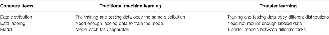
TABLE 1. The difference between ML and TL.
It should be known that TL-based methods have been utilized in many real applications, such as natural language processing, image classification, and pattern diagnosis (Lu et al., 2015; Patel et al., 2015). For example, based upon the FTL method, Long et al. (2014) proposed a method of joint matching with transfer (TMJ) and instance selection while minimizing the distribution distance. Jing et al., (2017) proposed different transformation matrices for the source domain and target domain to achieve the goal of transfer learning. Based on the MTL method, Zhao et al. (2011) proposed the Trans EMDT method, which uses a decision tree to build a robust behavior diagnosis model based on the labeled data. It should be known that limited research studies use the RTL method (Davis and Domingos, 2009). Besides, Ganin et al. (2016) proposed the DANN method, which adds a confrontation to train neural networks. Bousmalis et al. (2016) from Google Brain extended DANN by proposing a DSN network.
According to the abovementioned discussion, TL methods could well benefit the computational efficiency and diagnostic accuracy, which is promising to be used in the rolling bearing fault diagnosis of new energy vehicles. Driven by this, a novel data-driven method named the transfer-based deep neural network (DNN-TL) through integrating CNN, LSTM, and transfer learning is designed in this study. In the DNN-TL method, the characteristics and advantages of the algorithms are used to improve the overall performance of new energy vehicles’ fault diagnostics in terms of diagnostics accuracy and training efficiency. More specifically, CNNs and LSTM can intelligently extract preliminary features, but alleviate the complicated training and fine-tuning process of CNNs hyperparameters. Then, the preliminary features are refined, and the accuracy of the fault condition classification is enhanced by the TL algorithm with maximum mean discrepancy (MMD) and deep domain adaptation (DDA).
The logic of designing the DNN-TL method is detailed below: First, CNNs and LSTM are designed to extract fault-related features from the signals on a rolling bearing of new energy vehicles. To get the appropriate value of hyperparameters, the Grid Search method is improved, namely, step heapsort. Second, the excellent parameter model is saved for transfer learning. Moreover, the loss function is also improved by introducing MMD to optimize the features by eliminating those less relevant to faults. Finally, DDA is developed to fine-tune the extracted feature values to the target data for transfer learning and obtain the final fault diagnosis classification. Case studies with different complexities evince the superiority of the DNN-TL method in comparison with each of the individual base models and other existing TL approaches. The case studies also exemplify the industrial applicability of the DEL approach under real-world environments with noises and signal interferences.
The rest of this study is organized as follows. DNN-TL Method details the framework to derive the DNN-TL method. Experiments and Results illustrates the experiments and analyzes the corresponding results. Finally, conclusions are summarized and further applications, shortages, and challenges are discussed in Conclusion.
DNN-TL Method
Figure 1 illustrates the flowchart of the derived DNN-TL method. Specifically, Step 1 to Step 4 are used for feature extraction of the data set. Step 5 is to classify the data set. Step 6 is to show the evaluation index. After that, the comparison tests would be carried out to verify the effectiveness of the derived DNN-TL method.
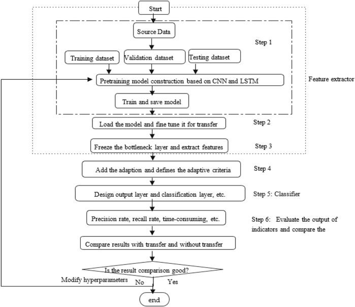
FIGURE 1. Flowchart of the DNN-TL approach.
Deep Neural Network Establishment
To observe a better pre-training model in rolling bearing fault diagnosis of new energy vehicles, this study proposes DCNNL by combining CNN and LSTM for pre-training, as illustrated in Figure 2. Specifically, first, after adding batch normalization (Szegedy et al., 2017b) between the convolutional layer and the pooling layer, the input would be pulled into the convolutional layer back forcibly to the standard normal distribution. This could avoid disappearing from the gradient, further speeding up the convergence and the training speed. Second, by adding the LSTM network (Chi et al., 2020; Landi et al., 2021) after the pooling layer, the long-term dependency problem (gradient explosion) could be solved to better refine the feature. Finally, a dropout layer is added to the fully connected layer for preventing overfitting and improving the generalization ability (Lei et al., 2020). The flowchart of DCNNL based on combined CNN and LSTM is shown in Figure 2.
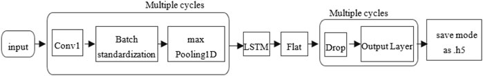
FIGURE 2. Flowchart of the model.
Raw Data Preprocess
To avoid the overfitting issue and increase the generalization ability of the entire network, the original data will be processed by data expansion (Wong et al., 2016), as illustrated in Figure 3. Here, a translational overlap sampling processing method through the sliding window overlap sampling is adopted for 2048 samples. The offset step size (S) is 28. The standard deviation is to standardize the data. Finally, the data encode is one-hot. Through this method, data set N has 620,544 data. Training samples are N- (L-S). According to the Andrew course (Zonneveld, 1994), the processed data sets include the training set, validation set, and test set. The ratio is of 7:2:1. In this context, overlap sampling can increase the data. Standardization makes each of the input close. The network can converge well. Hyperparameters are same for each training. The way can simplify processing hyperparameters later.
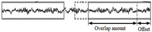
FIGURE 3. Translational overlap sampling method.
Design Hyperparameters of DNN
Deep neural networks (DNNs) have many parameters, which would have a great influence on performing the network. Figure 4 illustrates the types of these hyperparameters. The common hyperparameters include network structure, optimization parameters, and regularization coefficients. The parameter settings include manual search, grid search, and random search (Li et al., 2021d). An improved grid search method of step heapsort is utilized in this study. Table 2 illustrates the detailed procedure of this step heapsort method. Specifically, first, an initial value and maximum value are set for the parameters in the network. Second, a fixed step size is given to get the next parameter, while the result of the corresponding parameter is calculated. Third, the ideal result is obtained through using the Heapsort method. Finally, the computer automatically calculates the comparison result to get the idea hyperparameters.
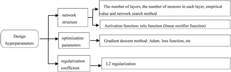
FIGURE 4. Types of related hyperparameters.
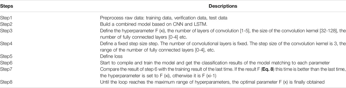
TABLE 2. Procedure of step heapsort.
The number of neurons in the layers, the size of convolution kernel, and the fully connected layer are obtained through the step heapsort method. The activation includes saturated and unsaturated functions (Testoni et al., 2017). The former can solve the gradient disappearance and speed up the convergence speed. The latter cannot. So, this study selects the unsaturated function. Unsaturated functions have ReLU and related variants. The methods of gradient descent include batch gradient descent (BGD), stochastic gradient descent (SGD), mini-batch gradient descent, AdaGrad, and Adam. Adam is better than other adaptive learning methods (Wang et al., 2010), so Adam is selected as the gradient descent method. The regularization coefficient L2 is adopted due to its smooth nature.
The choice of hyperparameters eventually needs the loss. The smaller the loss, the closer the predicted value from the model is to the true value. The loss mainly includes regression loss and classification loss. The choice of commonly used classification is illustrated in Table 3. Many faults belong to the multi-classification problem. Here, the activation for the output layer selects Softmax, and the loss is the cross-entropy loss. The formula is as follows:
where
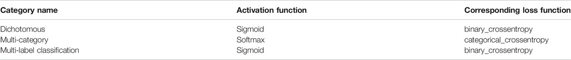
TABLE 3. Choices of classification function.
Considering the CNN and LSTM within the model, the loss function is improved as follows:
with
where
Model Training and Generation
The flowchart of model training is shown in Figure 5. Through the step heapsort method, accuracy rate, training time, and other parameters will be written into the array after each training. The next training can compare with the previous results to get the ideal hyperparameters of the model. Finally, the model is saved to promote the transfer of the model.
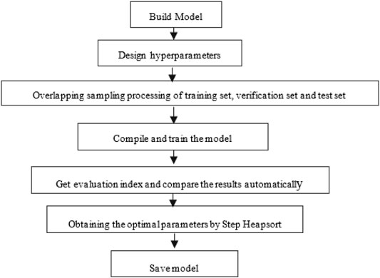
FIGURE 5. Flowchart of model training.
Transfer of the Pre-Trained Model
To find an ideal TL method, after the training model is built, the model in the source domain would be transferred to the target domain and fine-tuned. The fine-tuning of the pre-training model is to freeze the bottleneck layer of the model. The bottleneck layer is from the convolutional layer to the fully connected layer. It uses the weight of the pre-trained model to freeze the layer, extract the feature value of the target domain, and then, add in the source domain and the target domain adaptive layer. The flowchart of the transfer is shown in Figure 6A. The steps of fine-tuning are shown in Figure 6B. 1) Use the data of CWRU as the source data set. Then, train a deep neural network model DCNNL based on CNN + LSTM. Its specific is shown in Figure 6C. In the source model, the model has 18 layers. The previous 12 layers use three layers as a series: convolution, standardization, and maximum pooling. The 13th layer is to add the LSTM network, and the 14th layer is the Flatten layer; the 15th layer performs dropout processing on the Flatten layer. The 16th layer is a fully-connected layer. The 17th layer adds an activation, and the 18th layer is also a fully-connected layer for predicting classification. 2) Create the target model, and copy all the features of the source model except the penultimate fully-connected layer. 3) Add multiple fully-connected layers, add the actual number of target sets, and initialize the model parameters randomly. 4) Train the target model on the target data set, and then, train the classification results of the output layer from scratch. The parameters of other layers are fine-tuned based on the features of the source model.
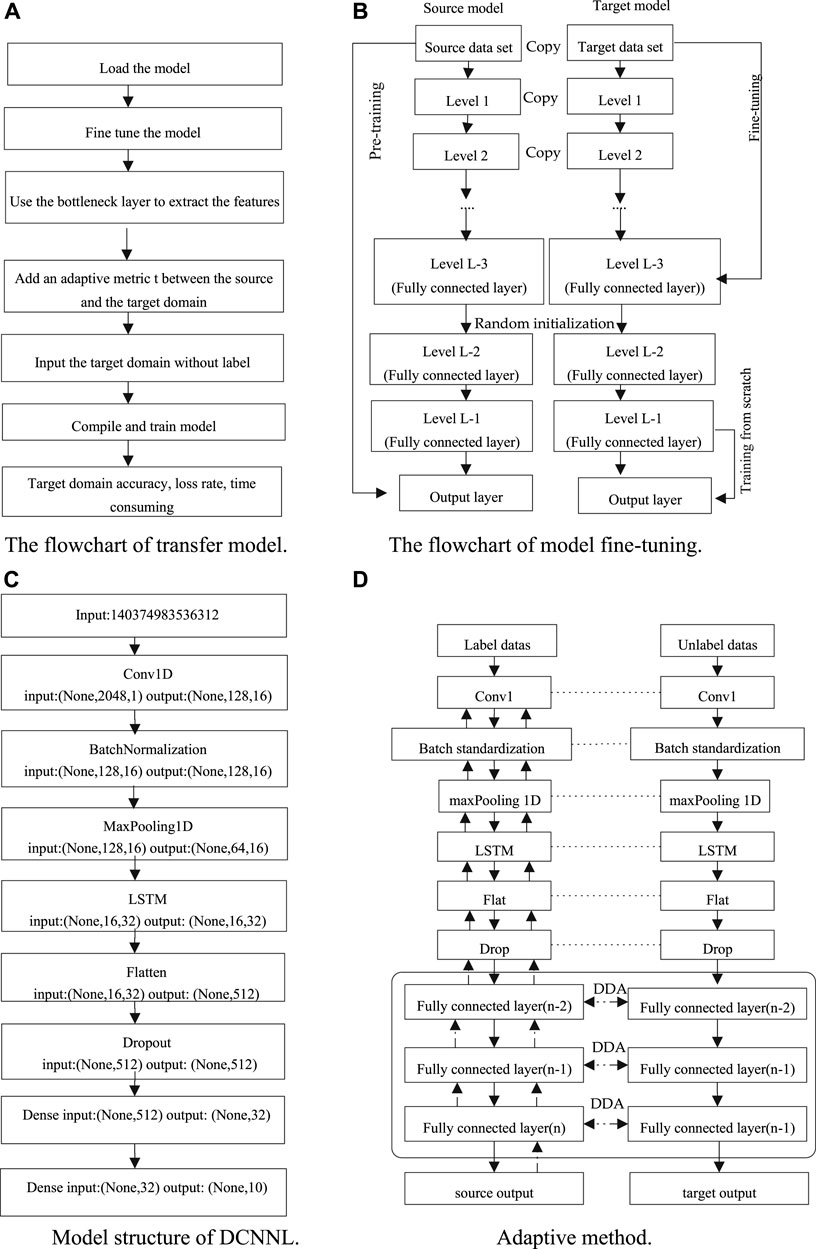
FIGURE 6. The transfer of model. (A) Flowchart of the transfer model. (B) Flowchart of model fine-tuning. (C) Model structure of DCNNL. (D) Adaptive method.
The deep network adaptation layer mainly completes two tasks: (i) Which layers can adapt? (ii) What measurement is for adaptation? The network adaptation method in this study is DDA. Feature extraction is from the bottleneck layer of the transfer model. A layer using an adaptive measurement criterion adds the first three layers of the classifier. The adaptive method is shown in Figure 6D. The paper uses the loss function to measure. The first is multi-class cross-entropy loss. The second half is MMD. The formula of loss is as follows (4) and (5).
Model Evaluation
Evaluation for classification issues is to explore model’s accuracy. To quantify model’s performance, the precision rate (P), recall rate (R), comprehensive evaluation index (F), and weighted average (weighted avg) are adopted. P and R is single induce. F takes both P and R into consideration. These evaluation metrics are described as follows:
where TP is true positive, FP is false positive, FN is false negative, SupportT is the support degree to reflect the actual number of positive categories in the data, and SupportF is another support degree to reflect the actual number of negative categories in the data.
Experiments and Results
Experimental Platform Construction and Data Preparation
To evaluate the effectiveness of the DNN-TL method in the diagnosis of new energy vehicles faults, the data set of Case Western Reserve University (CWRU) and the rolling bearing data set of the laboratory are utilized. Since rolling bearings are key components of new energy vehicles, an experimental platform shown in Figure 7A is used to collect vibration signals of rolling bearings. The platform is powered by a SEW DRE100M4/BE5/HF/V/FI motor. The specifications of the motor are as follows: the output power is 2.2 kW, the rated speed is 1,425 RPM, and the rated torque is 4 Nm. The rolling bearing is a 6,209 deep groove ball bearing. Its inner diameter is 45 mm, outer diameter is 85 mm, and width is 19 mm.
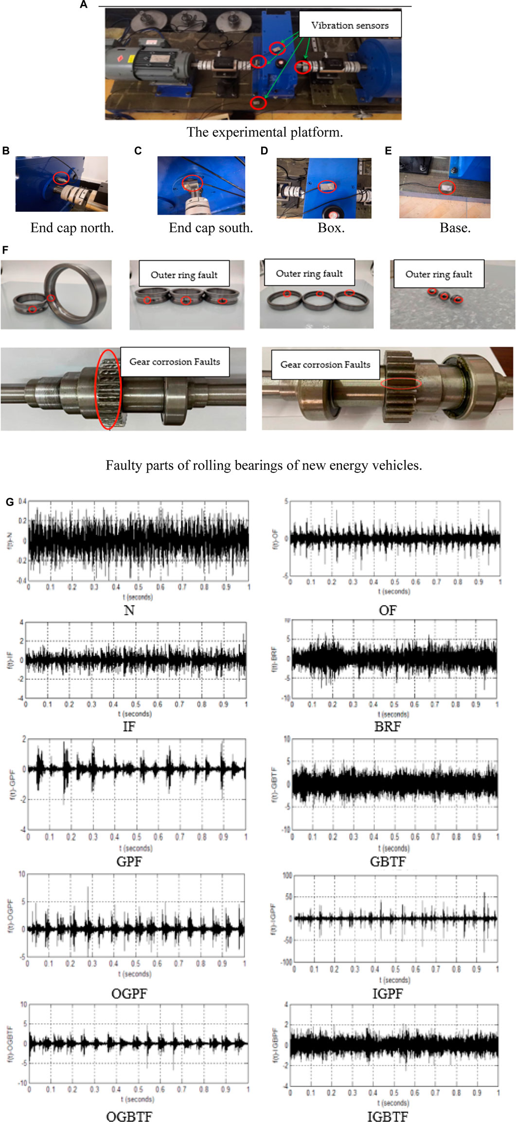
FIGURE 7. Experimental platform deployment. (A) The experimental platform, (B) end cap north, (C) end cap south, (D) box, (E) base, (F) faulty parts of rolling bearings of new energy vehicles, and (G) part of the original data.
The platform has different faults to verify the correctness of the prediction classification of the transfer model. They are the outer ring, inner ring, rolling, and gear of the bearing. To collect different fault signals, there are vibration acceleration sensors on the north of the end cover, the south of the end cover, the box, and the base. The locations of fault point sensors are shown in Figures 7B–E. Vibration signals of the rolling bearings were collected by four vibration sensors deployed on the platform at a sampling frequency of 10.24 kHz for each fault. The data sets include 10 faults in Table 4. The faults are normal (N), bearing outer ring fault (OF), bearing inner ring fault (IF), bearing rolling fault (BRF), gear pitting fault (GPF), gear broken tooth fault (GBTF), bearing outer ring and gear pitting fault (OGPF), bearing inner ring and gear pitting fault (IGPF), bearing outer ring and gear broken tooth fault (OGBTF), and bearing inner ring and gear broken tooth fault (IGBTF). The motor speed and load of different faults are shown in Table 4. There are 30 samples. Each sample is transformed into 1,000 samples using the transnational overlap sampling method. Each contains 1,024 sampling points. The training data set, the verification data set, and the test data set are divided into 700, 200, and 100, respectively. Figure 7G shows a typical part of the original data.
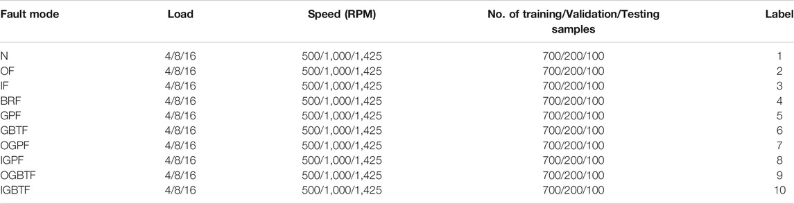
TABLE 4. Descriptions of the rolling bearing data set.
Experimental Results
To verify the versatility of the proposed pre-training model and the possibility of the transfer learning method, this study compares various methods.
The Comparison of the Results of Different Models Without Transfer
The study sets up seven models. They are DNN-TL, CNN, LSTM, DBN, AE, KNN, and SVM. The parameters of the model are shown in Table 5. The size of each model input is self-defined dimensions according to requirements. Training iteration is all set to 10,000. AE encoding layer is as 2048-128-64-10; decoding is the opposite of encoding. The weights of all points in each field of KNN are equal. The penalty parameter in SVM is C. It is 1.0 to get accuracy and generalization. Kernel is Gaussian kernel. The losses in CNN and LSTM are cross-entropy. This study improves the loss of DNN-TL, see Eq. 3. The data are collected by the test platform. The coefficients (
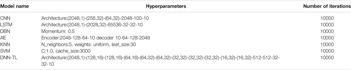
TABLE 5. The hyperparameters of different models.
The hyperparameters of DCNNL are trained by the step heapsort algorithm. Specifically, the data sets of CWRU are as the training data of the domain. Part of the training results are shown in Table 6, and the number of iterations is 11. The training time is at least 13 s, followed by 14 s, and the most is 27 s. The highest accuracy of the training set is 1, the highest accuracy of the validation set is 0.9925, and the lowest loss rates of the training set and validation set are 0.0026428 and 0.05091, respectively. For the shortest time-consuming 13 s, the accuracy rates of the training set and validation set of 3-Conv-32-filters-LSTM-0-dense are 1 and 0.987, and the loss rates are 0.009069 and 0.07128. In the highest accuracy rate of 1, 3-Conv-32-filters-LSTM-1-dense takes the smallest time to be 14 s and the accuracy rate of the validation set is 0.989. The loss rates of the training and validation sets are 0.0073519 and 0.06609, respectively. Considering comprehensively, the accuracy of the 3-Conv-32-filters-LSTM-1-dense training result is the highest with 100%, the loss rate is 0.007352, the lowest is 0.002643, and the time is shorter than 14 s, second only to the lowest 13 s. Considering the highest accuracy rate, 3-Conv-32-filters-LSTM-1-dense is as the transfer model of DNN-TL. So the structure is shown in Table 7.
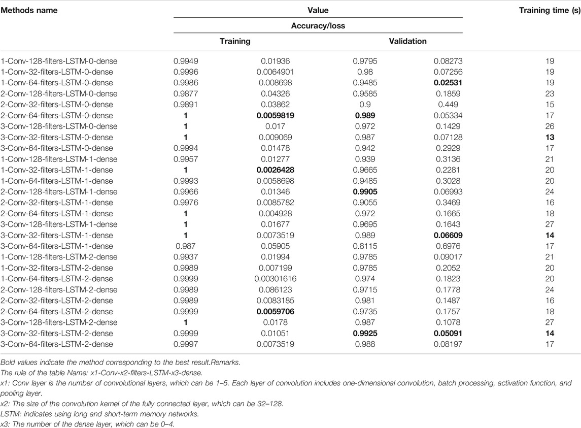
TABLE 6. Training accuracy, loss rate, and time consumption of the DCNNL model.
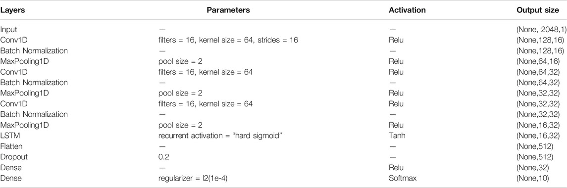
TABLE 7. DCNNL deep neural network topology map.
The experimental results are as follows. First, the average accuracy and time-consuming of the training set, validation set, and test set of the seven models are shown in Table 8A. These results are an average accuracy of 15 times. The results show that accuracy rates of DNN-TL in the training set, validation set, and the test set are 0.99977, 0.9998, and 0.987, respectively. The accuracy rates in the other six models without transfer are 0.9877, 0.8005, and 0.802. The standard deviations of DNN-TL are 0.32, 0.33, and 0.35, and the loss rates are 0.006469, 0.00067, and 1.6763. The minimum deviations of other models without transfer are 0.43, 0.52, and 0.68, and the loss rates are 0.0.0475, 0.1.6824, and 1.6863. The training time of DNN-TL is 18 s, while the lowest CNN of the other six models without transfer takes 20 s. So DNN-TL takes the shortest time, has the highest accuracy rate, and rather small deviation. This result shows the proposed method has a higher accuracy and robustness than other comparable methods in fault diagnosis. Since the DNN-TL model is trained with data from CWRU, it proves that this model has a strong ability to learn and has a good generalization.
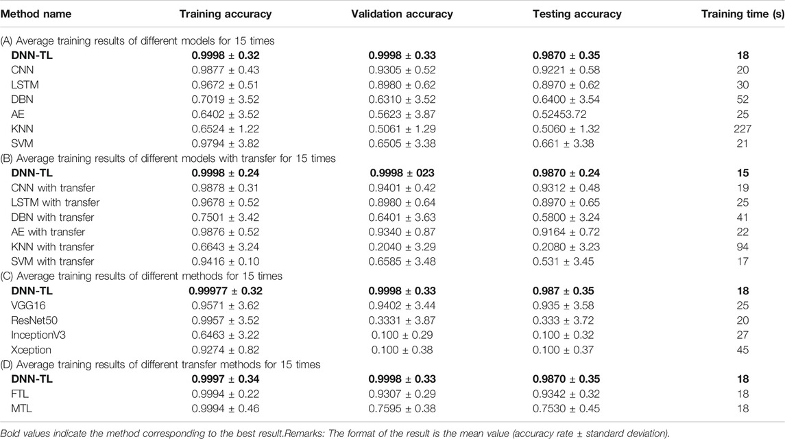
TABLE 8. 15 average training results of different methods.
Figure 8 shows the specific test accuracy of different methods in 15 experiments. In Figure 8, it shows that the accuracy of the DNN-TL model is the highest, which is close to about 99%, and the results are steady, while the results of the other six methods are low and unstable, and the robustness is not good. This result further shows the DNN-TL method is more accurate and more stable than the other six methods.
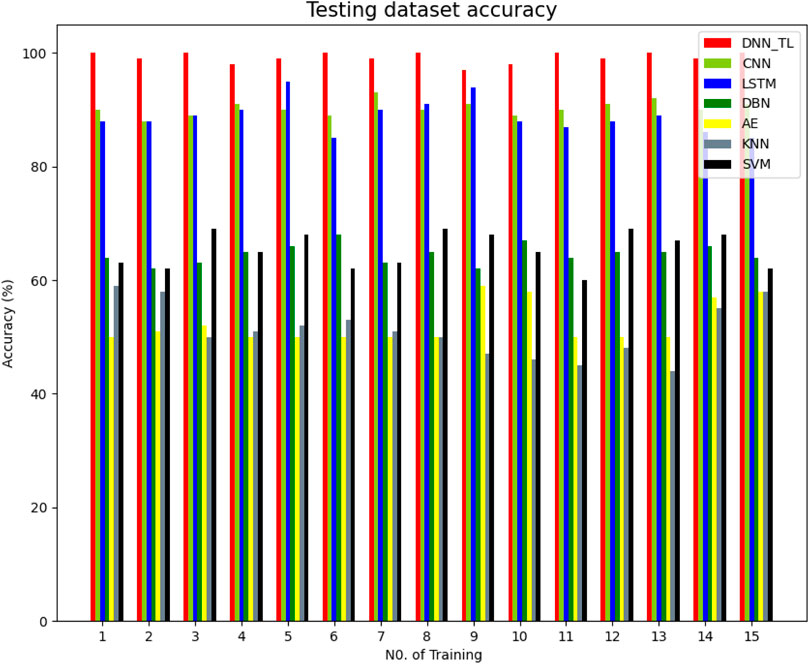
FIGURE 8. Accuracy rate of different methods in 15 experiments.
To further verify the proposed DNN-TL method, more specific experiments were tested. This study gets the P, R, F, and weighted avg of different methods. Figure 9A shows the accuracy of DNN-TL and the other six methods in the test set. The accuracy of DNN-TL is higher than that of other methods, especially in N, IF, OF, and GBTF. The accuracy of other methods is less than 60%. Among them, the diagnosis rate of KNN in most faults is low, not exceeding 40%, and the DNN-TL method reaches more than 95% and has a stable accuracy rate for all faults.
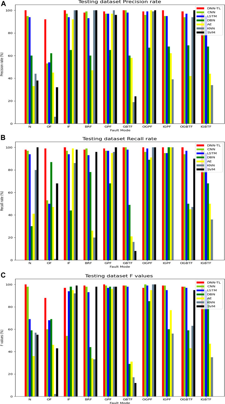
FIGURE 9. P, R, and F of different methods. (A) P; (B) R; and (C) F.
Figure 9B shows the recall rate of DNN-TL and six other methods on the test set. The recall rate of DNN-TL is higher than that of other methods, especially in N, IF, OF, BRF, OGPF, and IBGPF. And, the recall rate of other methods is less than 85%. The DNN-TL method reaches more than 95%.
Although the results of precision and recall are well displayed in the DNN-TL, they cannot evaluate a method comprehensively and objectively. Figure 9C shows the F of different methods. The value of F of the DNN-TL method is above 97% in different faults, especially in N, OF, IF, BRF, GBTF, and OGPF. The most in the other methods are less than 75%.
Table 9A shows the weighted avg of different P, R, and F, which can be clearly seen from the table. The weighted avg of DNN-TL is the highest, so the accuracy and stability of DNN-TL in the overall fault diagnosis are the best.
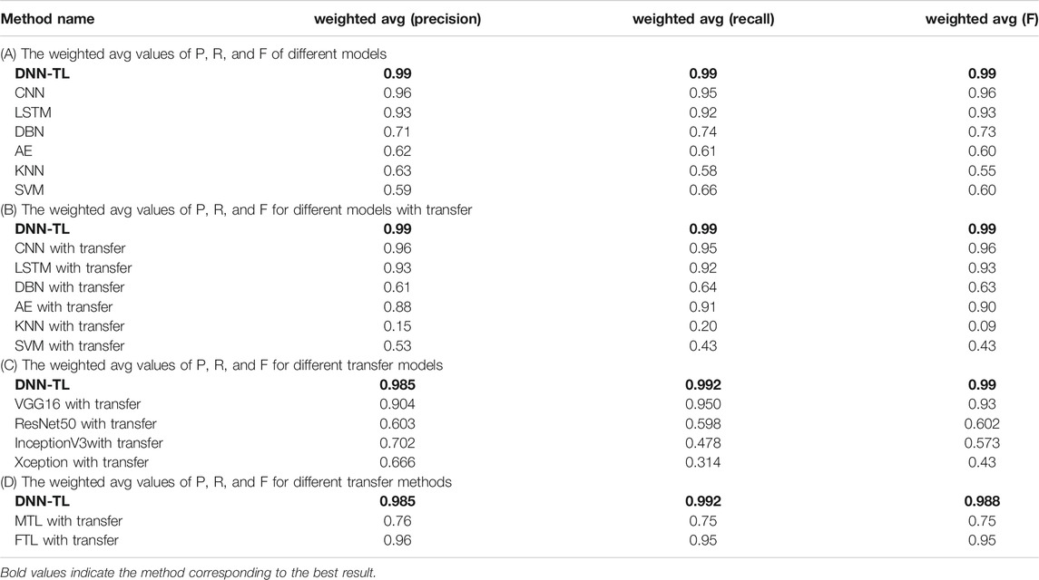
TABLE 9. The weighted avg values of P, R, and F of different methods.
Based on results, it can be implied the DNN-TL method can get higher accuracy, precision, recall, comprehensive evaluation indicators, and weighted avg. The results are more accurate, stable, and have generalization abilities. Besides, because it is transfer learning, the fine-tuning of the parameters simplifies the training time.
The Comparison of Results of Different Transfer Models
To further show the versatility, superiority, and feasibility of the model DNN-TL, the previous training methods of CNN, LSTM, DBN, AE, KNN, and SVM are kept as models, and the same transfer method is used for transfer. The experiment is performed on the same data set.
Table 8B shows the accuracy and time consumption of the training set, validation set, and test set 15 times. From Table 8A,B, it can be seen that the accuracy of the result after the transfer is better than that of the model without transfer; some have been reduced, and the overall time consumption has been shortened. The accuracy rates of the CNN, LSTM, DBN, AE, KNN, and SVM test sets without transfer is 0.9221, 0.8970, 0.6400, 0.5245, 0.5060, and 0.661, respectively; time consumption is 20 s, 30, 52, 25, 227, and 21 s. After transfer, the matching accuracy rate is 0.9312, 0.8970, 0.5800, 0.9164, 0.2080, and 0.531, and the time consumption is 19, 25, 41, 22, 94, and 17 s. It illustrates the versatility and feasibility of the DCCNLTL proposed in this study.
Figure 10, Figures 11A–C, and Table 9B respectively show the specific test accuracy, P, R, F, and weighted avg results of different transfer methods in 15 tests. On the test set, the effect of the DNN-TL method is overall higher than the results of other methods.
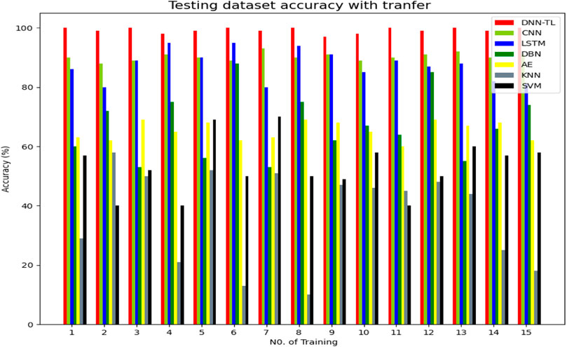
FIGURE 10. Accuracy of different transfer models.
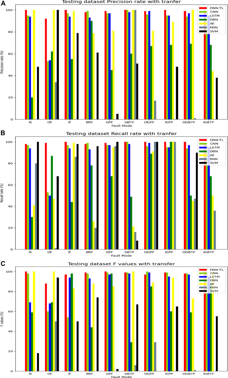
FIGURE 11. P, R, and F of different transfer models. (A) P; (B) R; and (C) F.
To further clarify what conditions can transfer learning and what conditions will have a negative transfer, this study uses mature models in other fields to experiment on the same data set.
The popular deep models are transferred, such as VGG16, ResNet50, InceptionV3, and Xception. The original data of these models are from Image net, which is not in the same field on the data set of this study. This directly fine-tunes and transfers this model to our experimental platform, using the alike measurement of DNN-TL, see Eq. 4. The training results are as follows.
Figures 12–14 and Table 8C show the accuracy and loss rate and time consumption of the training set, validation set, and test set 15 times. It shows that in the 6th training, DNN-TL can quickly achieve a high-accuracy rate of about 99%, and a low loss rate, which is close to about 0.007. The accuracy of the VGG16 method on the verification set in the 10th is relatively high at about 95%. The accuracy of other methods is very low, and the loss rate is very high. It shows the DNN-TL method can get better results in a short time and is convenient for rapid transfer. The time is about 18 s. The results are stable, and the accuracy is higher.
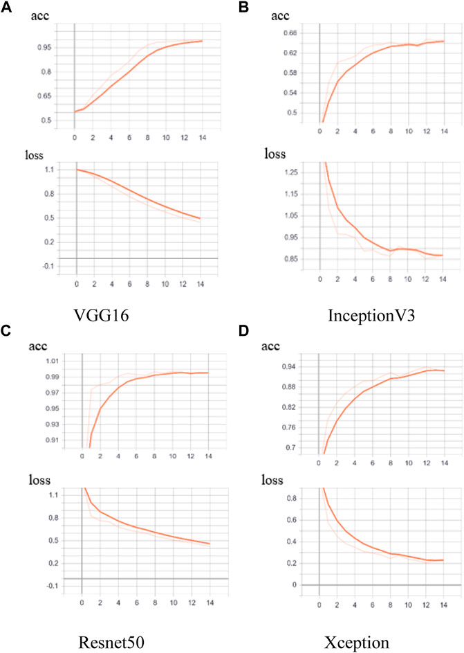
FIGURE 12. Accuracy and loss rate in the pre-trained model training set based on different models.
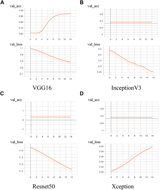
FIGURE 13. Accuracy and loss rate in the pre-trained model validation set on different models.
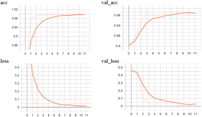
FIGURE 14. Accuracy and loss rate of training and validation sets based on DNN-TL pre-training.
To further verify the effect of the DNN-TL method, quantitative results of different methods are also explored and illustrated. In Figure 15A, the accuracy rate of DNN-TL reached above 95% except for the OF. The accuracy rate of N, IF, GBTF, and IGPF reached 100%. The transfer results of ResNet50, InceptionV3, and Xception were unstable, good, or bad. The accuracy rate of VGG16 with the transfer is about 80%, which is lower than DNN-TL, so the accuracy rate of DNN-TL is the highest and most stable.
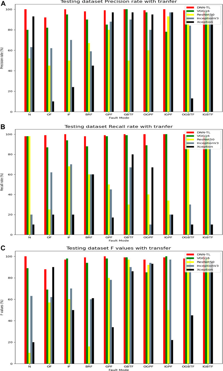
FIGURE 15. P, R, and F of different methods with transfer. (A) P; (B) R; and (C) F.
Similarly, in Figure 15B, the recall rate of DNN-TL is less than 90% except for OF, BRF, and OGPF. The other recall rates have reached more than 90%, while the recall rate of other methods is low and unstable.
According to Figure 15C, the F value of DNN-TL also presents the highest value.
Table 9C shows the weighted avg of P, R, and F. It can be clearly seen that the weighted avg in DNN-TL reaches more than 95%. VGG16 is higher than 90%, and other transfer models are less than 60%. Table 9A,C show in models, the highest weighted avg without transfer is 0.96 (CNN) and the lowest is 0.58 (KNN). In image-related transfer models, the weighted avg is the highest 0.93 (VGG16), and the minimum is 0.314 (Xception). The weighted avg in Table 9 is stable. In Table 9C, the weighted avg of P, R, and F is different. So, the accuracy rate in fault diagnosis is unstable.
The Comparison of the Results of Different Transfer Methods
Next, this study will further verify the accuracy and stability of the proposed DNN-TL in fault diagnosis. Because FTL and MTL are widely used, the DNN-TL uses MTL- and FTL-based transfer methods. This study compares DNN-TL and separate MTL- and FTL-based methods. The method based on MTL is to directly load the pre-trained model to predict the result. The FTL-based method is to extract the feature value of the Flatten layer of the pre-trained model as the input of the model, and then, add a fully connected layer for classification training.
Table 8D shows the accuracy and loss rate and time consumption on the training set, validation set, and test set 15 times. The time consumption of the three transfer methods is 18 s. The DNN-TL has the highest accuracy rate of 0.9997 and the lowest loss rate of 0.006469. The accuracy rate and loss rate of the other method verification sets are lower. So, the transfer method of DNN-TL is superior to the separate transfer methods such as FTL and MTL. The DNN-TL is convenient for rapid transfer and has stable results and high accuracy.
In Figure 16A, the accuracy rate in DNN-TL has reached 95% except for OF faults. The accuracy rates of N, IF, GBTF, and IGPF have reached 100%. The accuracy rates of FTL and MTL are only 100% in OF. So, overall the accuracy rate of DNN-TL is higher and more stable.
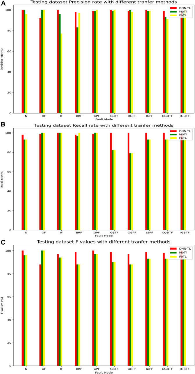
FIGURE 16. P, R, and F of the test set of different transfer methods. (A) P; (B) R; and (C) F.
Similarly, in Figure 16B, the recall rate of DNN-TL is more than 90% except OF, BRF, and OGPF. The recall rates in GBTF, OGPF, IGTF, OGBTF, and IGBTF based on MTL are 82, 79, 93, 93, and 93%, respectively. These based on FTL are 83, 79, 93, and 92%. The recall rate of DNN-TL is as high as 95%.
According to Figure 16C, the F value of DNN-TL, except that OF is lower than FTL and MTL methods, for the F value of other faults, DNN-TL is the highest.
Table 9D shows the weighted avg. The weighted avg of DNN-TL has reached more than 98%. FTL is 95%, and MTL is only 75%.
Experiment Analysis
Based upon the comparisons of the model without transfer, the model with transfer, and the different transfer methods, the following observations can be summarized: 1) It is obvious that the DNN-TL model is superior to other models with transfer, without transfer, and other transfer methods. It explains the relative versatility of the DNN-TL model. 2) Compared with models with transfer and without transfer, DNN-TL can get higher diagnosis results and does not need professional manual extraction of feature values. It directly uses original signal data, which reflects the advantages of unsupervised learning of deep transfer learning. 3) Compared with several other transfer models in different fields, the accuracy of DNN-TL on the training set and validation set is much higher than that in other models, and the loss rate is low. VGG16, ResNet50, InceptionV3, and Xception perform well in image and Visio. But these transfer models are poor in recognizing faults. The adaptive layer and the judgment between the source domain and the target domain are added before the classification layer of all transfer models. It can be concluded that the deep transfer learning cannot give full play to its advantages in unrelated fields. Even there may be a negative transfer. It also shows that the similarity domain judgment proposed in this study has a certain meaning. 4) Different transfer methods show that DNN-TL is better than the MTL and FTL methods alone.
The above conclusions show that DNN-TL l is in related or similar fields, and the likeness can be measured by certain rules. According to the loss rate of Table 8C, if the likeness should be less than 0.007, the accuracy of the transfer is better. At the same time, deep neural networks in feature extraction are better, and the possibility of negative transfer is reduced. The DNN-TL is better than the transfer method alone. So, the DNN-TL with combined adaptive deep transfer learning proposed in this study has certain general and advanced research significance in fault diagnosis.
Conclusion
In this study, to achieve an effective rolling bearing fault diagnosis of new energy vehicles for low carbon economy, a novel DNN-TL method is developed. Specifically, through extracting features by CNNs and LSTM, more effective features can be obtained in supporting new energy vehicles’ fault diagnostics. Besides, through assigning optimized MMD costs and DDA to different faults, the proposed DNN-TL could classify the fault conditions more accurately. According to the case studies of using different methods to validate the accuracy and robustness of the DNN-TL method, some conclusions can be observed as follows: 1) The pre-training model of DCNNL proposed can be used as a better model for feature extraction. 2) MTL- and FTL-based transfer methods that are used in classification issues (such as identifying fault categories) are also applicable. The combined transfer method is better than the individual transfer method. 3) The likeness judgment between the source domain and the target domain is a certain effect. 4) The step heapsort method can quickly and accurately determine the hyperparameters of the model and improve the model accuracy. 5) Areas with low likeness may not be suitable for deep transfer learning. As the remaining life prediction of new energy vehicles has not been considered in this study, our future work would focus on designing the automatic calculation of residual service life prediction in the later stage of bearing fault diagnosis research.
Data Availability Statement
The raw data supporting the conclusion of this article will be made available by the authors, without undue reservation.
Author Contributions
YW is responsible for providing experimental design, data analysis, and code implementation. WL is responsible for providing ideas.
Funding
This research was supported by the National Natural Science Foundation of China (Project No. 51975444) and an advanced manufacturing lab establishment funding supported by the Wuhan University of Technology.
Conflict of Interest
The authors declare that the research was conducted in the absence of any commercial or financial relationships that could be construed as a potential conflict of interest.
Publisher’s Note
All claims expressed in this article are solely those of the authors and do not necessarily represent those of their affiliated organizations, or those of the publisher, the editors, and the reviewers. Any product that may be evaluated in this article, or claim that may be made by its manufacturer, is not guaranteed or endorsed by the publisher.
Acknowledgments
The authors would also acknowledge the review comments from mentors WL and colleagues in the universities of the authors.
References
Bousmalis, K., Trigeorgis, G., Silberman, N., et al. (2016). Domain Separation Networks[J]. Adv. Neural Inf. Process. Syst. 29, 343–351.
Chen, Q., and Pan, G. (2021). A Structure-Self-Organizing DBN for Image Recognition. Neural Comput. Applic 33 (3), 877–886. doi:10.1007/s00521-020-05262-2
Chen, Z., Deng, S., Chen, X., Li, C., Sanchez, R.-V., and Qin, H. (2017). Deep Neural Networks-Based Rolling Bearing Fault Diagnosis. Microelectronics Reliability 75, 327–333. doi:10.1016/j.microrel.2017.03.006
Chi, Y., Yang, S., and Jiao, W. (2020). Multi-label Classification Method of Rolling Bearing Fault Based on LSTM-RNN[J]. J. Vibration, Measurement& Diagn. 40 (3), 563–629.
Chine, W., Mellit, A., Lughi, V., Malek, A., Sulligoi, G., and Massi Pavan, A. (2016). A Novel Fault Diagnosis Technique for Photovoltaic Systems Based on Artificial Neural Networks. Renew. Energ. 90, 501–512. doi:10.1016/j.renene.2016.01.036
Davis, J., and Domingos, P. (2009). “Deep Transfer via Second-Order Markov Logic[C],” in Proceedings of the 26th annual international conference on machine learning, 217–224.
Feng, H., Li, S., and Li, H. (2020). Identification of Key Lines for Multi-Photovoltaic Power System Based on Improved PageRank Algorithm[J]. Front. Energ. Res. 8, 341. doi:10.3389/fenrg.2020.601989
Ganin, Y., Ustinova, E., Ajakan, H., et al. (2016). Domain-adversarial Training of Neural Networks[J]. J. machine Learn. Res. 17 (1), 2096–2030.
Guo, X., Chen, L., and Shen, C. (2016). Hierarchical Adaptive Deep Convolution Neural Network and its Application to Bearing Fault Diagnosis. Measurement 93, 490–502. doi:10.1016/j.measurement.2016.07.054
Hoang, D.-T., and Kang, H.-J. (2019). A Survey on Deep Learning Based Bearing Fault Diagnosis. Neurocomputing 335, 327–335. doi:10.1016/j.neucom.2018.06.078
Hongcan, L. I. U., and Wang, X. (2021). Recent advance in Screening Lithium Solid-State Electrolytes through Machine Learning[J]. Front. Energ. Res. 9, 9.
Janssens, O., Slavkovikj, V., Vervisch, B., Stockman, K., Loccufier, M., Verstockt, S., et al. (2016). Convolutional Neural Network Based Fault Detection for Rotating Machinery. J. Sound Vibration 377, 331–345. doi:10.1016/j.jsv.2016.05.027
Jia, F., Lei, Y., Lin, J., Zhou, X., and Lu, N. (2016). Deep Neural Networks: A Promising Tool for Fault Characteristic Mining and Intelligent Diagnosis of Rotating Machinery with Massive Data. Mech. Syst. Signal Process. 72-73, 303–315. doi:10.1016/j.ymssp.2015.10.025
Jia, F., Lei, Y., Lin, J., Zhou, X., and Lu, N. (2016). Deep Neural Networks: A Promising Tool for Fault Characteristic Mining and Intelligent Diagnosis of Rotating Machinery with Massive Data. Mech. Syst. Signal Process. 72-73, 303–315. doi:10.1016/j.ymssp.2015.10.025
Jing, Z., Li, W., and Ogunbona, P. (2017). “Joint Geometrical and Statistical Alignment for Visual Domain Adaptation[C],” in CVPR.
Landi, F., Baraldi, L., Cornia, M., et al. (2021). Working Memory Connections for LSTM[J]. Neural Networks.
Lecun, Y., Bengio, Y., and Hinton, G. (2015). Deep Learning. Nature 521 (7553), 436–444. doi:10.1038/nature14539
Lei, Y., Yang, B., Jiang, X., Jia, F., Li, N., and Nandi, A. K. (2020). Applications of Machine Learning to Machine Fault Diagnosis: A Review and Roadmap. Mech. Syst. Signal Process. 138, 106587. doi:10.1016/j.ymssp.2019.106587
Li, G., Wang, W., Zhang, W., Wang, Z., Tu, H., and You, W. (2021). Grid Search Based Multi-Population Particle Swarm Optimization Algorithm for Multimodal Multi-Objective Optimization. Swarm Evol. Comput. 62, 100843. doi:10.1016/j.swevo.2021.100843
Li, J., Li, Y., and Yu, T. (2021). Temperature Control of Proton Exchange Membrane Fuel Cell Based on Machine Learning[J]. Front. Energ. Res., 582.
Li, R., Li, W., Zhang, H., Zhou, Y., and Tian, W. (2021). On-Line Estimation Method of Lithium-Ion Battery Health Status Based on PSO-SVM[J]. Front. Energ. Res., 401.
Li, S., Siu, Y. W., and Zhao, G. (2021). Driving Factors of CO2 Emissions: Further Study Based on Machine Learning[J]. Front. Environ. Sci., 323.
Liu, K., Hu, X., Meng, J., et al. (2021). RUBoost-Based Ensemble Machine Learning for Electrode Quality Classification in Li-Ion Battery Manufacturing[J]. IEEE/ASME Trans. Mechatronics.
Liu, K., Hu, X., Zhou, H., et al. (2021). Feature Analyses and Modelling of Lithium-Ion Batteries Manufacturing Based on Random forest Classification[J]. IEEE/ASME Trans. Mechatronics.
Liu, K., Shang, Y., Ouyang, Q., and Widanage, W. D. (2020). A Data-Driven Approach with Uncertainty Quantification for Predicting Future Capacities and Remaining Useful Life of Lithium-Ion Battery[J]. IEEE Trans. Ind. Electron. 68 (4), 3170–3180. doi:10.1109/TIE.2020.2973876
Long, M., Wang, J., Ding, G., Sun, J., and Yu, P. S. (2014). “Transfer Joint Matching for Unsupervised Domain Adaptation,” in CVPR, 1410–1417. doi:10.1109/cvpr.2014.183
Lu, J., Behbood, V., Hao, P., Zuo, H., Xue, S., and Zhang, G. (2015). Transfer Learning Using Computational Intelligence: A Survey. Knowledge-Based Syst. 80, 14–23. doi:10.1016/j.knosys.2015.01.010
Patel, V. M., Gopalan, R., Li, R., and Chellappa, R. (2015). Visual Domain Adaptation: A Survey of Recent Advances. IEEE Signal. Process. Mag. 32 (3), 53–69. doi:10.1109/msp.2014.2347059
Ren, H., Hou, Z. J., Vyakaranam, B., Wang, H., and Etingov, P. (2020). Power System Event Classification and Localization Using a Convolutional Neural Network[J]. Front. Energ. Res. 8, 327. doi:10.3389/fenrg.2020.607826
Rui, Z., Yan, R., Chen, Z., Maob, K., Wangc, P., and Gaoc, R. X. (2019). Deep Learning and its Applications to Machine Health Monitoring[J]. Mech. Syst. Signal Process. 115, 213–237.
Schmidhuber, J. (2015). Deep Learning in Neural Networks: An Overview. Neural networks 61, 85–117. doi:10.1016/j.neunet.2014.09.003
Shao, H., Jiang, H., Wang, F., and Zhao, H. (2017). An Enhancement Deep Feature Fusion Method for Rotating Machinery Fault Diagnosis. Knowledge-Based Syst. 119, 200–220. doi:10.1016/j.knosys.2016.12.012
Shao, H., Jiang, H., Zhang, X., and Niu, M. (2015). Rolling Bearing Fault Diagnosis Using an Optimization Deep Belief Network. Meas. Sci. Technol. 26 (11), 115002. doi:10.1088/0957-0233/26/11/115002
Shao, H., Jiang, H., Zhao, H., and Wang, F. (2017). A Novel Deep Autoencoder Feature Learning Method for Rotating Machinery Fault Diagnosis. Mech. Syst. Signal Process. 95, 187–204. doi:10.1016/j.ymssp.2017.03.034
Shujaat, M., Wahab, A., Tayara, H., and Chong, K. T. (2020). pcPromoter-CNN: A CNN-Based Prediction and Classification of Promoters. Genes 11 (12), 1529. doi:10.3390/genes11121529
Syaifullah, A. H., Shiino, A., Kitahara, H., et al. (2021). Machine Learning for Diagnosis of AD and Prediction of MCI Progression from Brain MRI Using Brain Anatomical Analysis Using Diffeomorphic Deformation[J]. Front. Neurol. 11, 1894. doi:10.3389/fneur.2020.576029
Szegedy, C., Ioffe, S., Vanhoucke, V., et al. (2017). “Inception-v4, Inception-Resnet and the Impact of Residual Connections on Learning[C],” in Thirty-first AAAI conference on artificial intelligence.
Szegedy, C., Ioffe, S., Vanhoucke, V., et al. (2017). “Inception-v4, Inception-Resnet and the Impact of Residual Connections on Learning[C],” in Thirty-first AAAI conference on artificial intelligence.
Testoni, R., Levizzari, R., and De Salve, M. (2017). Coupling of Unsaturated Zone and Saturated Zone in Radionuclide Transport Simulations. Prog. Nucl. Energ. 95, 84–95. doi:10.1016/j.pnucene.2016.11.012
Wang, C., Han, F., Zhang, Y., and Lu, J. (2020). An SAE-Based Resampling SVM Ensemble Learning Paradigm for Pipeline Leakage Detection. Neurocomputing 403, 237–246. doi:10.1016/j.neucom.2020.04.105
Wang, C., Wang, D.-Z., and Lin, J.-L. (2010). ADAM: An Adaptive Multimedia Content Description Mechanism and its Application in Web-Based Learning. Expert Syst. Appl. 37 (12), 8639–8649. doi:10.1016/j.eswa.2010.06.089
Wang, H., Xu, J., Yan, R., Sun, C., and Chen, X. (2020). Intelligent Bearing Fault Diagnosis Using Multi-Head Attention-Based CNN. Proced. Manufacturing 49, 112–118. doi:10.1016/j.promfg.2020.07.005
Weiss, K., Khoshgoftaar, T. M., and Wang, D. D. (2016). A Survey of Transfer Learning[J]. J. Big Data 3 (1), 1–40. doi:10.1186/s40537-016-0043-6
Wong, S. C., Gatt, A., Stamatescu, V., et al. (2016). “Understanding Data Augmentation for Classification: when to Warp? [C],” in 2016 international conference on digital image computing: techniques and applications (DICTA) (Gold Coast, QLD, Australia: IEEE), 1–6.
Zhang, W., Li, C., Peng, G., Chen, Y., and Zhang, Z. (2018). A Deep Convolutional Neural Network with New Training Methods for Bearing Fault Diagnosis under Noisy Environment and Different Working Load. Mech. Syst. Signal Process. 100, 439–453. doi:10.1016/j.ymssp.2017.06.022
Zhao, Z., Chen, Y., Liu, J., et al. (2011). “Cross-People Mobile-Phone Based Activity Diagnosis[C],” in International Joint Conference on Artificial Intelligence (Palo Alto, California, U.S.: AAAI Press).
Keywords: low carbon energy applications, deep learning, transfer learning, fault diagnosis, energy vehicle
Citation: Wang Y and Li W (2021) Transfer-Based Deep Neural Network for Fault Diagnosis of New Energy Vehicles. Front. Energy Res. 9:796528. doi: 10.3389/fenrg.2021.796528
Received: 17 October 2021; Accepted: 08 November 2021;
Published: 14 December 2021.
Edited by:
Kailong Liu, University of Warwick, United KingdomReviewed by:
Run Fang, Wuhan University, ChinaYing Gao, The University of Electro-Communications, Japan
Huang Aibin, Hangzhou Dianzi University, China
Copyright © 2021 Wang and Li. This is an open-access article distributed under the terms of the Creative Commons Attribution License (CC BY). The use, distribution or reproduction in other forums is permitted, provided the original author(s) and the copyright owner(s) are credited and that the original publication in this journal is cited, in accordance with accepted academic practice. No use, distribution or reproduction is permitted which does not comply with these terms.
*Correspondence: Weidong Li, d2VpZG9uZ2xpQHdodXQuZWR1LmNu