Maximizing frequency security margin via conventional generation dispatch and battery energy injection

1 Introduction

Renewable energy sources, notably inverter-connected wind turbines (Xiao et al., 2021; Wei et al., 2022) and photovoltaic solar power, usually do not provide synchronous inertia. The increasing integration of renewable energy sources deteriorates the primary frequency response (Doherty et al., 2010; Ingleson and Allen, 2010; Sharma et al., 2011; Illian, 2017), as synchronous units with governor supplying frequency response are replaced by asynchronous renewable units that contribute little to synchronous inertia and governor response. In this context, the traditional assumptions that synchronous inertia is sufficiently high and governor response is adequate are not always valid, especially under light load and high renewable generation (Eto et al., 2010). Therefore, it becomes more critical to evaluate whether a system can maintain frequency stability following disturbances.

In current practices, simulations are performed under some typical operation modes to examine whether frequency stability requirements are met (Illian, 2017). However, frequency dynamics are closely related to pre-disturbance power dispatch (O’Sullivan and O’Malley, 1996; Doherty et al., 2005; Chávez et al., 2014), equipment characteristics, the disturbance and frequency response provided by fast-acting resources such as battery energy storage system (BESS) (Lian et al., 2017; Zhang et al., 2018; Engels et al., 2020; Golpîra et al., 2020). It is thus challenging to determine the best frequency stability level that a system can achieve through simulation methods. To quantitatively evaluate the maximum frequency stability margin of a system, an appropriate evaluation metric and an effective evaluation method are necessary.

Frequency nadir (the minimum value of frequency) is an important metric for assessing frequency stability (Rezkalla et al., 2018). Simulations are performed in O’Sullivan and O’Malley (1996) to calculate the frequency nadir for a given dispatch to check whether the frequency nadir limit constraint is satisfied. Egido et al. (2009) calculates frequency nadir using a simplified model that includes the regulation speed of governors. Oskouee et al. (2020)derives frequency nadir based on a multi-area system freaquency response model. In Uriarte et al. (2015), reaction time is first proposed to assess frequency stability, which is calculated as a function of microgrid ramp rate magnitudes and local inertia. Zhang et al. (2020) proposes the concept of frequency security margin which is defined as the maximum power imbalance that the system can tolerate. Although the above assessment metrics are utilized for frequency stability assessment, few studies have considered the impact of various control mechanisms, including the dispatch of conventional generation and battery energy injection schedule, on the assessment metrics.

To relate frequency nadir to pre-disturbance generation dispatch, our previous work Zhao et al. (2021) employs a set of discretized differential algebraic equations (DAEs) to express dynamic frequency response in a frequency stability constrained optimal re-dispatch model. It is a beneficial attempt to establish the connections between frequency dynamics and control mechanisms.

In this paper, a frequency nadir based margin metric, frequency security margin (FSM), is developed to quantitatively measure the frequency stability margin. A new dynamic frequency response constrained optimal power flow (DFR-OPF) that incorporates the dynamic frequency response similar to Zhao et al. (2021) is proposed to maximize FSM. DFR-OPF can make the most possible out of system frequency response capability to obtain the maximum frequency stability margin by optimizing the pre-disturbance conventional generation dispatch and battery energy injection schedule.

This paper mainly focuses on under-frequency events, such as those due to loss of generation, because they are more common. The main contributions of the paper are summarized as follows.

• This paper presents an optimization method to evaluate the maximum frequency stability margin considering the power dispatch of conventional units and the schedule of BESS energy injection.

• A smoothing method is developed to incorporate the intentional governor deadbands with negative frequency deviation inputs into an optimization framework.

• A metric is proposed to assess the safety margin and guide the enhancement of the delivered primary frequency response.

• A graphical tool is provided for region-wise frequency stability assessment. It suggests whether frequency stability for the current operating condition with a post-disturbance BESS scheduling can be improved and how much improvement is possible.

The remainder of this paper is organized as follows. Section 2 includes the mathematical model of dynamic frequency response for conventional generating units and BESS. In Section 3, the DFR-OPF model is presented to calculate the maximum of FSM. Section 4 introduces the region-wise graph for frequency stability assessment. The effectiveness of the proposed optimization method is validated in Section 5. Finally, conclusions are drawn in Section 6.

2 Dynamic frequency response model of conventional generating units and discussion on frequency support from BESS

2.1 Generic dynamic model of synchronous generating units governing frequency

The power deficit in a power system, caused by a sudden generation loss, is bound to cause drops in the rotor speed of synchronous units. For synchronous unit i ∈ S_SG, its frequency dynamics can be stated by the swing equations as follows:

$\frac{\mathrm{d}{\delta }_i}{\mathrm{d}t}={\omega }_i-{\omega }_{\text{n}}(1)$

$\frac{\mathrm{d}{\omega }_i}{\mathrm{d}t}=\frac{{\omega }_{\text{n}}}{2H_i}\left(P_{\text{m},i}-P_{\text{e},i}\right),(2)$

where S_SG is the set of the buses that the synchronous units are connected to, δ_i and ω_i are respectively the rotor angle and rotor speed, ω_n is rated synchronous speed, H_i is inertia constant (s), P_m,i is mechanical power of a turbine governor, P_e,i is electromagnetic power of a generator.

As to the electromagnetic power for unit i ∈ S_SG, the following expressions can be used to calculate it:

${\widehat{P}}_{\text{e},i}-\frac{E_i{\widehat{V}}_i\text{sin}\left({\delta }_i-{\widehat{\theta }}_i\right)}{X_{\text{d},i}^{\prime }}=0(3)$

${\widehat{Q}}_{\text{e},i}+\frac{{\widehat{V}}_i^2}{X_{\text{d},i}^{\prime }}-\frac{E_i{\widehat{V}}_i\text{cos}\left({\delta }_i-{\widehat{\theta }}_i\right)}{X_{\text{d},i}^{\prime }}=0,(4)$

where E_i is the constant voltage behind a transient reactance $X_{\text{d},i}^{\prime }$, ${\widehat{V}}_i$ and ${\widehat{\theta }}_i$ are respectively the post-disturbance voltage magnitude and the phase angle for bus i, and Q_e,i is the reactive power output for the unit connected to bus i.

The post-disturbance voltage variables ${\widehat{V}}_i$ and ${\widehat{\theta }}_i$ in 3, 4, i ∈ S_N, i ≠ l, are determined by the following post-disturbance network equations:

$\sum _{j=1}^n{\widehat{V}}_i{\widehat{V}}_j{Y}_{ij}\text{cos}\left({\widehat{\theta }}_i-{\widehat{\theta }}_j-{\alpha }_{ij}\right)+P_{\text{d},i}\left(f_s\right)-{\widehat{P}}_{\text{e},i}=0(5)$

$\sum _{j=1}^n{\widehat{V}}_i{\widehat{V}}_j{Y}_{ij}\text{sin}\left({\widehat{\theta }}_i-{\widehat{\theta }}_j-{\alpha }_{ij}\right)+Q_{\text{d},i}\left(f_s\right)-{\widehat{Q}}_{\text{e},i}=0(6)$

$f_s-\frac{{\sum }_{i=1}^{ng}{\omega }_i{H}_i}{2\pi {\sum }_{i=1}^{ng}{H}_i}=0,(7)$

where $Y_{ij}{e}^{j{\alpha }_{ij}}$ is the entry of the admittance matrix, f_s is the average frequency which is defined in (7) using the center of inertia method (Kundur et al., 1994), P_d,i(f_s) and Q_d,i(f_s) are respectively active and reactive load both expressed as functions of the average frequency, S_N is the set of all buses, and the generation loss is assumed to occur at bus l.

The variation of mechanical power is the direct result of the governor response. To derive the analytical expression of mechanical power, the differential algebraic equations expression of the block diagram for individual governor turbine is needed. There could be generators with different kinds of turbines. Here, The block diagram of a reheated steam turbine in Kundur et al. (1994) shown in Figure 1 is taken as an example to discuss how to formulate the dynamics of turbine governing systems. The boiler pressure is assumed to be constant in this paper. For i ∈ S_SG, i ≠ l, the frequency regulation mechanism of the reheated steam turbine in Figure 1 can be described as:

$\frac{\mathrm{d}{z}_{\text{g}1,i}}{\mathrm{d}t}=\frac{1}{T_{\text{G},i}}\left(K_{\text{G},i}\left({\omega }_i-{\omega }_{\text{n}}\right)-z_{\text{g}1,i}\right)(8)$

$\frac{\mathrm{d}{z}_{\text{g}2,i}}{\mathrm{d}t}=\frac{1}{T_{\text{CH},i}}\left(P_{\text{m0},i}-z_{\text{g}1,i}-z_{\text{g}2,i}\right)(9)$

$\frac{\mathrm{d}{z}_{\text{g}3,i}}{\mathrm{d}t}=\frac{1}{T_{\text{RH},i}}\left(z_{\text{g}2,i}-z_{\text{g}3,i}\right)(10)$

$P_{\text{m},i}-\left(1-F_{\text{HP},i}\right)z_{\text{g}3,i}-F_{\text{HP},i}{z}_{\text{g}2,i}=0,(11)$

where T_G,i, T_CH,i, T_RH,i are time constants, z_g1,i, z_g2,i, and z_g3,i are output variables of integrators, K_G,i is the slope of the droop characteristic equal to the reciprocal of the governor droop, P_m0,i is scheduled mechanical power, and F_HP,i is fraction of total turbine power.

FIGURE 1

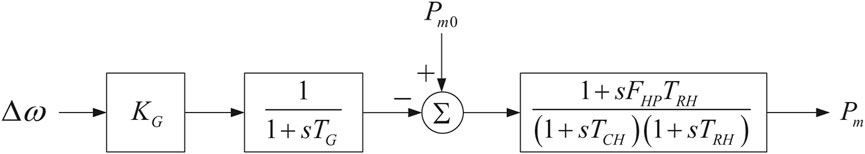
FIGURE 1. Block diagram of a reheated steam turbine.

Besides, the initial condition equations need to be considered in the frequency dynamic studies. For i ∈ S_SG, we have

${\omega }_i^0=2\pi f_0(12)$

$E_i{V}_i\text{sin}\left({\delta }_i^0-{\theta }_i\right)-P_{\text{g},i}{X}_{\text{d},i}^{\prime }=0(13)$

$V_i^2-E_i{V}_i\text{cos}\left({\delta }_i^0-{\theta }_i\right)+Q_{\text{g},i}{X}_{\text{d},i}^{\prime }=0,(14)$

where ${\omega }_i^0$ and ${\delta }_i^0$ are the pre-disturbance rotor speed and rotor angle for the unit connected to bus i, f₀ is the normal frequency, V_i and θ_i are pre-disturbance voltage magnitude and phase angle for bus i, P_g,i and Q_g,i are the scheduled active and reactive power of the unit connected to bus i. Eqs 1–4, 13, 14 develop a relationship between pre-disturbance generation dispatch and frequency dynamics.

2.2 Discretization of dynamic frequency response model expressed as DAEs

In Section 2.1, the dynamic frequency response of a synchronous generating unit is modeled as a set of DAEs. To incorporate these DAEs into an optimization problem, a numerical integration method is required to convert the DAEs to numerically equivalent algebraic equations.

Eqs 1–11 can be written in a general form as:

$\dot{\mathit{u}}={\mathcal{H}}_{\text{d}}\left(\mathit{u},\mathit{y}\right)(15)$

$\mathit{0}{=\mathcal{H}}_{\text{a}}\left(\mathit{u},\mathit{y}\right),(16)$

where u is the vector of the state variables, including δ_i, ω_i, z_g1,i, z_g2,i and z_g3,i. y is the vector of algebraic variables, including P_m,i, P_e,i, E_i, ${\widehat{V}}_i$ and ${\widehat{\theta }}_i$. ${\mathcal{H}}_{\text{d}}$ is the fuctional vector on the right hand side of differential Eqs 1, 2, 8–10. ${\mathcal{H}}_{\text{a}}$ is the fuctional vector of algebraic Eqs 3–7, 11.

As an example, using the trapezoidal rule for 15, 16 yields:

${\mathit{u}}^k-{\mathit{u}}^{k-1}=\frac{h}{2}\left({\mathcal{H}}_{\text{d}}\left({\mathit{u}}^k,{\mathit{y}}^k\right)+{\mathcal{H}}_{\text{d}}\left({\mathit{u}}^{k-1},{\mathit{y}}^{k-1}\right)\right)(17)$

$\mathit{0}{=\mathcal{H}}_{\text{a}}\left({\mathit{u}}^k,{\mathit{y}}^k\right),(18)$

where k = 1⋯, nt is the integration step counter, nt is the number of integration steps, and h is the integration step size. Note that the integration time T = h ∗ nt is set according to the duration of primary frequency regulation.

The dynamic frequency response model of synchronous units is discretized as a set of algebraic equations corresponding to different time through 17, 18, which enables us to dynamically track frequency response performance of in an optimization problem.

2.3 Smoothing of intentional governor deadband

Governor deadbands generally fall into two categories: unintentional and intentional deadband. The unintentional governor deadband is used to describe the inherent mechnical effect of a turbine governor system and is often represented as a backlash. The technical progress and improvement of the governor systems reduce the need to consider backlash (Illian, 2017). An intentional governor deadband adopted in modern governor designs can reduce excessive activity of controls and turbine mechanical wear for normal system frequency variations. In power systems, there are two types of intentional deadband, step deadband (SD) and non-step deadband (NSD). In this paper, only the implementations of non-step governor deadbands with negative frequency deviation inputs are considered to respond to under-frequency events.

The output of an non-step deadband is shown as:

$y_{\text{nsd}}=\left\{\begin{array}{cc}\hfill 0& -D<x\le 0\hfill \\ \hfill x+D& x\le -D\hfill \end{array}\right..(19)$

Note that (19) is not differentiable at some point, which will make an optimization model difficult to solve due to the incorporation of this expression. In this paper a smoothed non-step deadband (SNSD) is developed to smooth (19) as follows:

$y_{\text{nsd}}=\frac{x+D}{1+e^{\sigma \left(x+D\right)}}.(20)$

Figure 2 shows the curves of NSD and SNSD. Equation 20 allow the incorporation of non-step governor deadbands into an optimization problem as constraints.

FIGURE 2

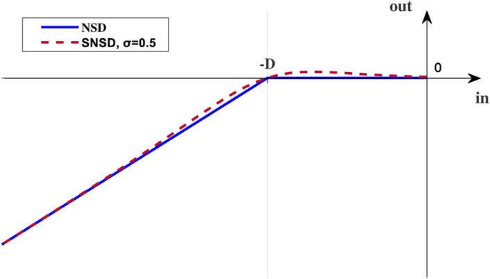
FIGURE 2. Non-step deadband and its smoothing.

2.4 Frequency support provided by BESS

Since this paper focuses on dynamic frequency response for under-frequency events, BESS is assumed only to inject power to the grid but not absorb energy to recover the state of charge of batteries during primary frequency control period. The discharge power of a BESS is considered as an adjustable variable in the proposed optimization problem of this paper and should be within the limits as follows:

$P_{\text{bsmin},i}\le P_{\text{bs},i}^k\le P_{\text{bsmax},i},i\in {\mathrm{S}}_{\mathrm{SE}},k=1\cdots ,nt,(21)$

where $P_{\text{bs},i}^k$ denotes the discharge power of the BESS integrated into Bus i at time k, P_bsmin,i and P_bsmax,i are respectively the upper and lower limit of discharge power, and S_ES is the set of the buses where BESSs are integrated.

The amount of energy a BESS should provide to support frequency during primary frequency response, ES_f,i, is thus:

$E{S}_{f,i}=\sum _{k=1}^{nt}{P}_{\text{dis},i}^{k}h,i\in {\mathrm{S}}_{\text{ES}}.(22)$

In Section 5 we will show that the energy that the batteries inject to provide frequency support is very small compared to their overall energy. Therefore the state of charge of batteries within the primary frequency control time frame is not discussed in this study.

3 DFR-OPF model for solving maximum frequency security margin

3.1 DFR-OPF formulation

We define FSM as the difference between the system frequency nadir and the allowable frequency lower limit:

$\mathrm{F}\mathrm{S}\mathrm{M}=f_{\text{nadir}}-f_{\text{all}},(23)$

where f_nadir and f_all denote system frequency nadir and allowable frequency lower limit respectively. System frequency nadir f_nadir refers to the minimum of frequency nadirs for all generators. Allowable frequency lower limit is the frequency at which load shedding occurs, commonly corresponding to the highest UFLS threshold. FSM represents a safety margin to ensure frequency stability. If FSM >0, the system can maintain frequency stability following a disturbance. Large FSM implies a high level of frequency stability. If FSM ≤0, UFLS may be trigged once a certain disturbance occurs. FSM helps operators know how much safety margin a system has, while the other frequency security related indicators cannot provide this information.

We propose a dynamic frequency response constrained OPF (DFR-OPF) model to obtain the maximum FSM (MFSM). In DFR-OPF, inertial and governor response are mathematically expressed as a set of differential algebraic equations (DAEs), allowing frequency response performance tracking. Two types of under-frequency events, generation loss and load increase, can be considered in the DFR-OPF model.

The objective of DFR-OPF is to maximize FSM.

The constraints of the DFR-OPF formulation include the dynamic frequency response constraints of conventional turbine generators and discharge power limits of BESS, in addition to regular limitations of classical OPF, such as full network power balance relations, technical restrictions, etc.

1. Nodal power balance relations under normal operations: Active and reactive power flow equations under normal operation are written as follows:

$\sum _{j=1}^n{V}_i{Y}_{ij}{V}_j\text{cos}\left({\theta }_i-{\theta }_j-{\alpha }_{ij}\right)+P_{\text{d},i}-P_{\text{g},i}=0(24)$

$\sum _{j=1}^n{V}_i{Y}_{ij}{V}_j\text{sin}\left({\theta }_i-{\theta }_j-{\alpha }_{ij}\right)+Q_{\text{d},i}-Q_{\text{g},i}=0(25)$

$\mathrm{f}\mathrm{o}\mathrm{r}i\in {\mathrm{S}}_{\text{N}}.$

Note that P_g,i = Q_g,i = 0 for the bus where there is no conventional power generation.

2. Swing equations and its related parameters expression: The swing equations in differential form are shown as 1, 2. To include them as constraints, 1, 2 are converted to a set of equivalent algebriac equations according to (17):

${\delta }_i^k-{\delta }_i^{k-1}=\frac{h}{2}\left({\omega }_i^k+{\omega }_i^{k-1}-2{\omega }_{\text{n}}\right)(26)$

${\omega }_i^k-{\omega }_i^{k-1}=\frac{h{\omega }_{\text{n}}}{4H_i}\left(P_{\text{m},i}^k+P_{\text{m},i}^{k-1}-P_{\text{e},i}^k-P_{\text{e},i}^{k-1}\right)(27)$

$\mathrm{f}\mathrm{o}\mathrm{r}i\in {\mathrm{S}}_{\text{SG}},i\ne l,k=1,\dots ,nt.$

If the under-frequency event is a generation loss, it is assumed that the conventional synchronous units connected to bus l are tripped off. And $P_{\text{e},i}^k$ can be expressed in the following form according to (3) and (18):

$P_{\text{e},i}^k=\frac{E_i{\widehat{V}}_i^k\text{sin}\left({\delta }_i^k-{\widehat{\theta }}_i^k\right)}{X_{\text{d},i}^{\prime }}(28)$

$\begin{array}{ll}\hfill & \mathrm{f}\mathrm{o}\mathrm{r}i\in {\mathrm{S}}_{\text{SG}},i\ne l,k=1,\dots ,nt.\hfill \\ \hfill & P_{\text{e},l}^k=0\mathrm{f}\mathrm{o}\mathrm{r}k=1,\dots ,nt.\hfill \end{array}(29)$

3. Post-disturbance nodal power balance relations: The post-disturbance nodal power balance equations should be discretized according to (18) and then represented by the following expressions with the consideration of the frequency support from BESS and two types of possible under-frequency events.

$\begin{array}{ll}\hfill & \sum _{j=1}^n{\widehat{V}}_i^k{Y}_{ij}{\widehat{V}}_j^k\text{cos}\left({\widehat{\theta }}_i^k-{\widehat{\theta }}_j^k-{\alpha }_{ij}\right)+P_{\text{d},i}\left(f_s\right)\hfill \\ \hfill & +\mathrm{\Delta }{P}_{\text{d},i}-P_{\text{e},i}^k-P_{\text{dis},i}^k=0\hfill \end{array}(30)$

$\begin{array}{ll}\hfill & \sum _{j=1}^n{\widehat{V}}_i^k{Y}_{ij}{\widehat{V}}_j^k\text{sin}\left({\widehat{\theta }}_i^k-{\widehat{\theta }}_j^k-{\alpha }_{ij}\right)+Q_{\text{d},i}\left(f_s\right)\hfill \\ \hfill & +\mathrm{\Delta }{Q}_{\text{d},i}-Q_{\text{e},i}^k=0\hfill \end{array}(31)$

$\mathrm{f}\mathrm{o}\mathrm{r}i\in {\mathrm{S}}_{\text{N}},k=1,\dots ,nt,$

where ΔP_d,i and ΔQ_d,i are the active and reactive load increase at Bus i. If the disturbance is a generation loss, ΔP_d,i = ΔQ_d,i = 0. If the disturbance is a load increase, no generation loss occurs at Bus l. P_dis,i = 0 if no BESS inject power to bus i. $Q_{\text{e},i}^k$ can be expressed in the following form according to (4) and (18):

$Q_{\text{e},i}^k=-\frac{{\left({\widehat{V}}_i^k\right)}^2}{X_{\text{d},i}^{\prime }}+\frac{E_i{\widehat{V}}_i^k\text{cos}\left({\delta }_i^k-{\widehat{\theta }}_i^k\right)}{X_{\text{d},i}^{\prime }}(32)$

$\begin{array}{ll}\hfill & \mathrm{f}\mathrm{o}\mathrm{r}i\in {\mathrm{S}}_{\text{SG}},i\ne l,k=1,\dots ,nt.\hfill \\ \hfill & Q_{\text{e},l}^k=0\mathrm{f}\mathrm{o}\mathrm{r}k=1,\dots ,nt.\hfill \end{array}(33)$

4. Dynamic frequency response of turbine governors: Based on their block diagrams, the frequency response for turbine governors can be expressed as a set of DAEs and then transformed to the following discrete form:

${\mathit{u}}_{\text{tg}}^k-{\mathit{u}}_{\text{tg}}^{k-1}=\frac{h}{2}\left({\mathcal{H}}_{\text{tg,\hspace{0.17em}d}}\left({\mathit{u}}_{\text{tg}}^k,{\mathit{y}}_{\text{tg}}^k\right)+{\mathcal{H}}_{\text{tg,\hspace{0.17em}d}}\left({\mathit{u}}_{\text{tg}}^{k-1},{\mathit{y}}_{\text{tg}}^{k-1}\right)\right)(34)$

$\mathit{0}{=\mathcal{H}}_{\text{tg,\hspace{0.17em}a}}\left({\mathit{u}}_{\text{tg}}^k,{\mathit{y}}_{\text{tg}}^k\right)(35)$

$\mathrm{f}\mathrm{o}\mathrm{r}k=1,\dots ,nt,$

where u_tg and y_tg are the state variable vector and the algebraic variable vector for turbine governors, and ${\mathcal{H}}_{\text{tg,\hspace{0.17em}d}}$ and ${\mathcal{H}}_{\text{tg,\hspace{0.17em}a}}$ are the differential equation vector and algebraic equation vector for turbine governors.

5. Operational and technical constraints: Before the disturbance occurs, the nodal voltage magnitude, the generating power and the current of lines are bounded by:

$V_{\text{min},i}\le V_i\le V_{\text{max},i},i\in {\mathrm{S}}_{\text{N}}(36)$

$P_{\text{gmin},i}\le P_{\text{g},i}\le P_{\text{gmax},i},i\in {\mathrm{S}}_{\text{SG}}(37)$

$Q_{\text{gmin},i}\le Q_{\text{g},i}\le Q_{\text{gmax},i},i\in {\mathrm{S}}_{\text{SG}}(38)$

$I_{ij}^2\le I_{\text{max},ij}^2,\left(i,j\right)\in S_{\text{Line}},(39)$

where I_ij is the current of line (i, j) and S_Line is the set of transmission lines.

Following an under-frequency event, the conventional generators increase their active power injection through speed governing systems. The incremental mechanical power of individual turbine generator should keep positive throughout primary frequency control:

$P_{\text{g},i}\le P_{\text{m},i}^k,i\in {\mathrm{S}}_{\text{SG}},i\ne l,k=1,\dots ,nt.(40)$

When a disturbance occurs, BESS begins to inject power to compensate for the power deficit. The discharging power limit constraint (21) should also be included.

6. Frequency nadir constraints: Since it is difficult to identify which unit contributes system frequency nadir and what time it is reached, this paper enforces unit frequency at every integration time above system frequency nadir, as expressed by:

$\frac{{\omega }_i^k}{2\pi }\ge f_{\text{nadir}},i\in {\mathrm{S}}_{\text{SG}},k=1\cdots ,nt.(41)$

Note that only the constraint with unit frequency at some time equal to system frequency nadir is bounded. Therefore, constraint (41) helps find out system frequency nadir in an indirect way.

7. Rate of change of frequency (ROCOF) constraints: It is necessary to ensure that ROCOF for all generators will not exceed the allowed upper limit, as shown below:

$\frac{{\omega }_i^{k-1}-{\omega }_i^k}{2\pi }\le {\mathrm{R}}_{\text{lim}}^{\text{cf}},i\in {\mathrm{S}}_{\text{SG}},k=1\cdots ,nt,(42)$

where ${\mathrm{R}}_{\text{lim}}^{\text{cf}}$ is the allowed maximum ROCOF. Note that the ROCOF throughout primary frequency regulation is considered. The ROCOF is enforced like this because the maximum ROCOF for individual generator does not always emerge immediately following the disturbance.

Thus, the DFR-OPF model is summarized as follows:

max FSM

s.t. 24–27, 30–31, 34–42.

Any well-developed nonlinear programming algorithms can be used to effectively solve this problem.

3.2 Allocation of primary reserves

The primary reserves allocated to the units responsible for governor response can be obtained based on the solution of the proposed DFR-OPF model. The primary reserve for each conventional unit is considered as the maximum of the incremental mechanical power output of the turbine during primary frequency control interval, expressed by:

$\begin{array}{ll}\hfill P_{\text{r},i}=\underset{k=1,\dots ,nt}{\text{max}}& \left(P_{\text{m},i}^k\right)-P_{\text{g},i},\hfill \\ \hfill & i\in {\mathrm{S}}_{\text{SG}},i\ne l,k=1,\dots ,nt,\hfill \end{array}(43)$

where P_r,i is the primary reserve for the unit integrated in Bus i. Allocating primary reserves among all conventional units based on (43) promises to arrest frequency decline after an under-frequency event and to recover frequency partially before second frequency control works.

4 Region-wise graph for frequency security assessment

Based on MFSM, this section provides a graphical tool to enable region-wise frequency stability assessment. The tool is appliable to both generation loss and load increase event.

A sudden under-frequency event, caused by generation loss or load increase, will lead to a power deficit. For a certain under-frequency event, varying its power deficit can produce a set of event scenarios. For those event scenarios, the proposed DFR-OPF model is run many times to explore the variation of MFSM under different values of power deficit. The curve of MFSM under different power deficit values is shown in Figure 3 as the dotted curve. Then, the point where MFSM is zero can be located on the curve. The power deficit value corresponding to this point is the maximum allowable imbalance power (MAIP) that a system can endure. Finally, three regions can be obtained as shown in Figure 3.

• The green part with FSM above zero represents the stable region. If the point corresponding to a current operating condition with an appropriate post-disturbance BESS scheduling falls in this region, it indicates that the current operating condition can maintain frequency stability if the BESS follows the post-disturbance scheduling.

• The blue part with FSM below zero and power deficit less than MAIP is called the correctable region. Although the FSMs in the correctable region are negative, the frequency stability level in this region could be improved and pushed to the stable region through re-dispatching the power generation of conventional units and re-scheduling the BESS power injection. The proposed DFR-OPF model can give an optimal power generation resdispatch and BESS power reschedule to move a point from the blue region to a location at the edge of the green region with the same power deficit, as shown in Figure 3.

• The red part with FSM below zero and power deficit greater than MAIP is the unstable region. If a power deficit exceeds MAIP, the system cannot maintain frequency stability following the disturbance. Furthermore, no dispatch operation through re-dispatching generation power and re-scheduling BESS power injection can make the system go back to the stable region.

FIGURE 3

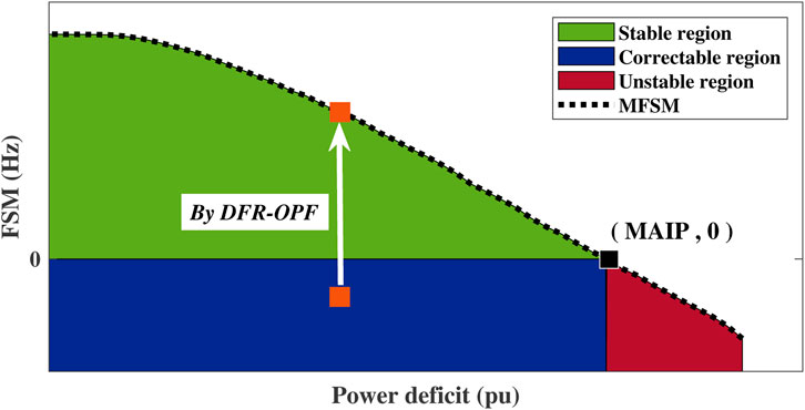
FIGURE 3. Region-wise graph for frequency security assessment.

The region-wise graph can provide operators situational awareness of the frequency stability and guide them to take actions when necessary. Specifically, the operators should first calculate FSM for a given conventional generation dispatch and BESS power schedule under an anticipated under-frequency event through time-domain simulation. If the obtained FSM falls in the stable region, the operating condition with the BESS power schedule is acceptable to resist the under-frequency event. If the obtained FSM falls in the correctable region, the operators could employ the proposed DFR-OPF model to maximize FSM, eventually obtaining the most reliable conventional generation dispatch and BESS power schedule. If the obtained FSM falls in the unstable region, the operators should first consider enhancing the primary frequency response of the online conventional generators. A simple way is to start up more generators with large inertia constants. To decide the additional generators to start in an optimal way, the unit commitment model in Restrepo and Galiana (2005)considering frequency stability constraints can be solved .

5 Case studies

5.1 WSCC 3-machine 9-bus system

The WSCC 3-machine 9-bus system and New England 10-machine 39-bus system are used to validate the FSM metric and the effectiveness of the proposed optimization method. All traditional generators are thermal power units. Their governors are modeled as the WSCC Type G governor (Power World Corporation, 2022) as shown in Figure 4, and the power limit in turbine-governing system is handled as Zhao et al. (2021). To exclude the impact of the variations of active load power and network loss on system frequency to facilitate analysis, all loads are formulated as constant power loads and the resistance of the transmission lines and transformers are ignored. The DFR-OPF model is formulated in GAMS and solved using the IPOPTH solver (Wächter and Biegler, 2006). All calculations are performed on a HP EliteOne 800 computer with a four-core 3.2-GHz processor and 8-GB RAM memory.

FIGURE 4

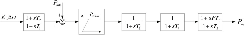
FIGURE 4. The block diagram of the WSCC Type G governor.

The system data of the WSCC 3-machine 9-bus system in Sauer and Pai (1997) are used here. Table 1 shows the characteristics and technical parameters of turbine governors and generators. Other parameters for calculations are given in Table 2. A BESS is supposed to be integrated to bus 4, and its rated power and rated energy capacity are the same. A sudden load increase (LI) is assumed to occur at bus 5.

TABLE 1

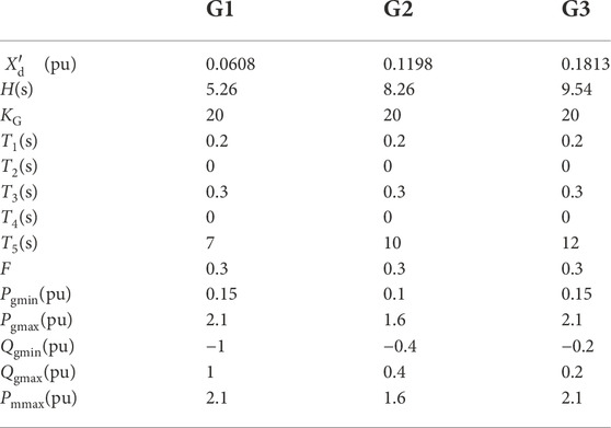
TABLE 1. Parameters of generators and turbine governors for WSCC 9-bus system.

TABLE 2

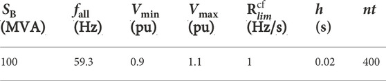
TABLE 2. Other parameters for calculation in 9-bus system.

Figure 5 shows the region-wise graphs with and without BESS participating in frequency regulation. It can be observed that the stable region is enlarged with the help of frequency support from BESS. It implies that the frequency stability capability is enhanced. And the increase of MAIP from 0.3694 pu to 0.4404 pu indicates the system’s improved ability to resist under-frequency events.

FIGURE 5

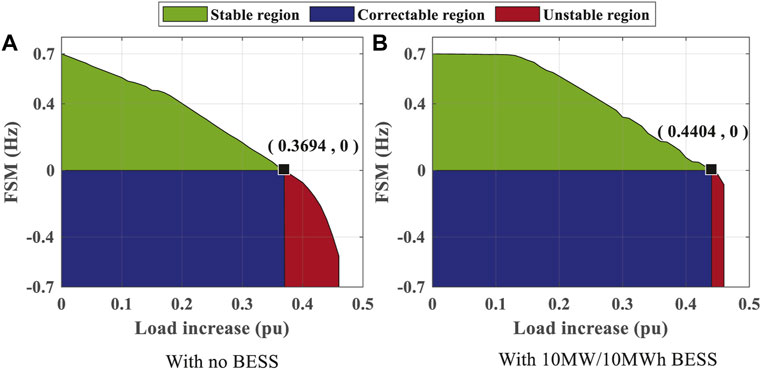
FIGURE 5. A comparison of two region-wise graphs between with no BESS and with 10 MW/10 MWh BESS.

Figure 6 illustrates the variation of MFSM with the rated power of BESS under different load increase events. The value of MFSM grows as the rated power of BESS increases under the same amount of LI. It implies that the more power capacity a BESS has, the higher level of frequency stability a system can achieve. Figure 6 also shows that small LI yields large MFSM for the same BESS rated power. It indicates that the less the imbalance power is, the stronger capability to ensure frequency security a system has.

FIGURE 6

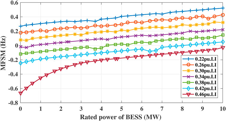
FIGURE 6. The variation of MFSM with the rated power of BESS following different load increase events.

Figure 7A illustrates the average frequency under different BESSs providing frequency support. As BESS’s rated power increases, the average frequency nadir increases and the rate of change of frequency decreases. It is due to the effect of the virtual inertia and the frequency response from BESSs. The total electromagnetic power (Total Pe) of all the conventional generators decreases with the increase of the BESS rated power as shown in Figure 7B, because the BESS with higher rated power injects more power into the system to help compensate the power deficit. It is noted that the total electromagnetic power during primary frequency control may include one or several sudden increase. It is probably due to the time-space distribution characteristics of frequency (Jin et al., 2019). Actually, the electromagnetic power for each generator shows oscillational change. The sum of those oscillational changes may easily come into being sudden increase. Figure 7C privides the changes of BESS discharge power (DP) with time. It is seen that BESS begins to discharge power immediately after the disturbance and provides frequency support throughout primary frequency regulation. Note that BESS does not keep discharging power without interruption, for the total electromagnetic power include sudden increase. Moreover, only a small amount of BESS energy is needed to participate in frequency regulation during primary frequency control, as shown in Figure 7D.

FIGURE 7

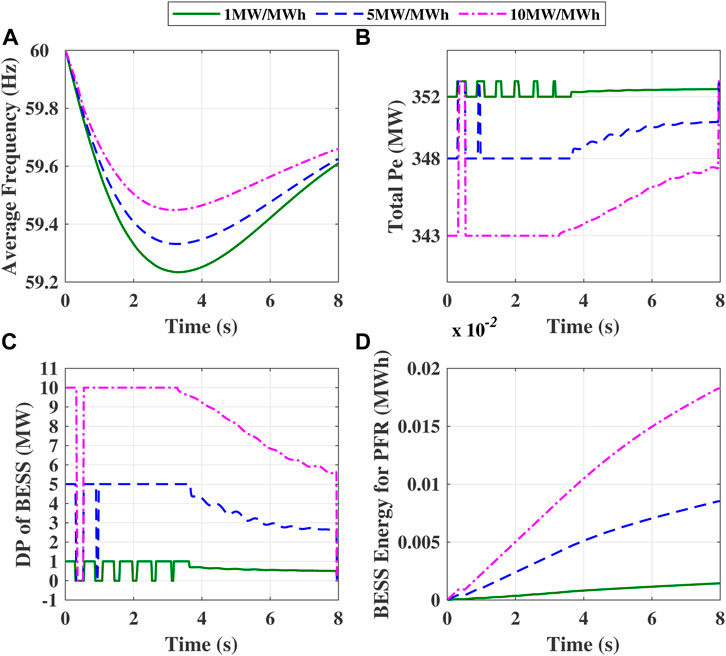
FIGURE 7. Curves (average frequency curve, total Pe curve, DP of BESS curve and BESS energy for PFR curve) for different BESSs providing power injection for the load increase of 0.38 pu.

The impact of a non-step deadband on frequency stability is then discussed here. Figure 8 shows the effect of changing the governor non-step deadband on average frequency and MFSM for a 0.34 pu load increase when a 10MW/10 MWh BESS participating frequency regulation. Compared to the results for no deadband, the non-step deadband reduces the frequency stability level. A smaller deadband ensures a stronger capability of arresting frequency decline and offering a larger frequency security margin.

FIGURE 8

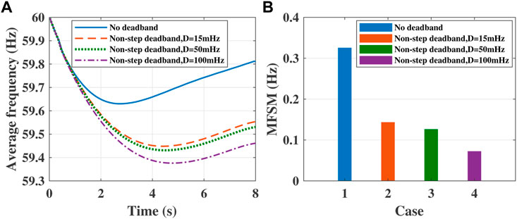
FIGURE 8. The effects of non-step deadbands on average frequency and MFSM.

5.2 New England 10-machine 39-bus system

The New England 10-machine 39-bus system has ten generators to be dispatched, but only G1-G9 can provide governor response to respond to a frequency deviation. The network data can be found in Pai (1989). Parameters of generators and turbine governors are listed in Tables 3, 4. The parameters for calculation are in Table 5. It is assumed that a sudden generation loss occurs due to G1 tripping off. A BESS is integrated into bus 10 to participate in frequency regulation.

TABLE 3

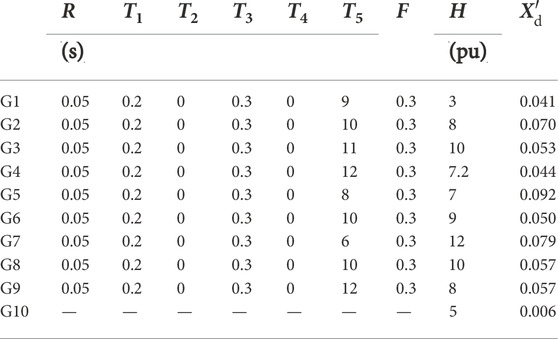
TABLE 3. Parameters of turbine governors and generators for 39-bus system.

TABLE 4

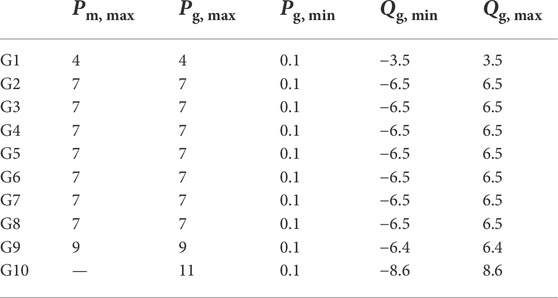
TABLE 4. Technical parameters in per unit for 39-bus system.

TABLE 5

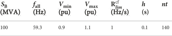
TABLE 5. Other parameters for calculation in 39-bus system.

Since unit frequencies are different from each other following an under-frequency event, not all units reach the minimum frequency nadir. Here, we call the units with the minimum frequency nadir critical-frequency units. According to FSM’s definition, the critical-frequency units play a decisive role on FSM. To study FSM from the point of view of individual units, we define unit FSM as the difference of unit frequency nadir, not system frequency nadir, from the allowable frequency lower limit. Figure 9 shows the unit FSMs following different generation losses without power injection from BESS. For generation losses of 0.86 pu, 0.91 pu, 0.96 pu, 1 pu, the critical-frequency units are marked by stars. It is observed that the combinations of the critical-frequency units are not the same under different generation losses. When a 10 MW/10 MWh BESS injects energy to the system, the enhanced capability to ensure frequency stability is observed in Figure 10. And the combination of the critical-frequency units changes after considering the BESS power injection under the same generation loss. This observation is consistent with the time-space distribution characteristic of frequency (Jin et al., 2019).

FIGURE 9

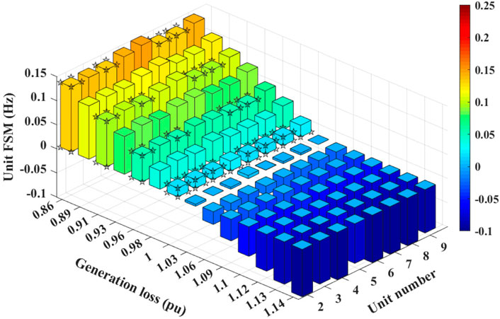
FIGURE 9. Unit frequency stability margin with no integration of BESS.

FIGURE 10

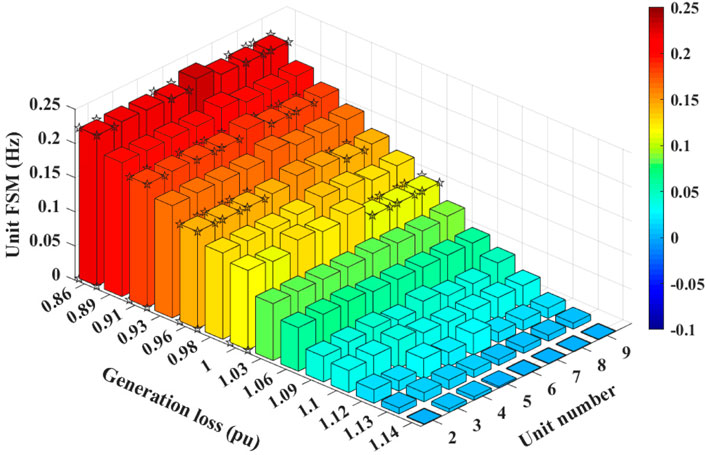
FIGURE 10. Unit frequency stability margin with a 10 MW/10 MWh BESS providing frequency support.

It can be seen from Table 6 that the incorporation of BESS brings a different pre-disturbance dispatch compared to the results for no BESS injection following the same generation loss of 1.00 pu. The pre-disturbance power dispatch needs to be adjusted to adapt to the integration of BESS. Then the primary preserves for all units, P_r,i in (43), are decreased due to the power injection of the BESS following the disturbance.

TABLE 6

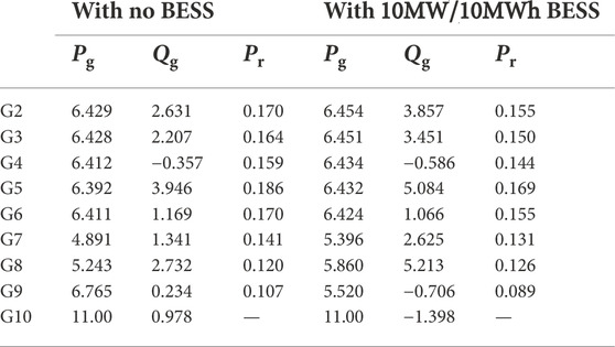
TABLE 6. Generation power dispatch and primary reserve in per unit.

Figure 11 shows the average frequency curves under different levels of inertial response for the generation loss of 1.00 pu. When the inertia constant H for all generators are reduced by 30%, the average frequency curve’s descent speed increases, and the average frequency nadir decreases. To increase the average frequency nadir to the original level and still satisfy the ROCOF limits, an 8.6 MW/8.6 MWh BESS is needed to be integrated into bus 10 to participate in frequency regulation. BESS can effectively prevent the deterioration of frequency stability caused by insufficient inertial response capability.

FIGURE 11

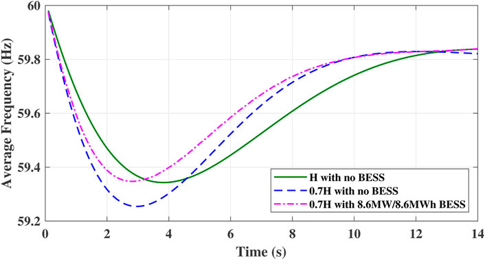
FIGURE 11. The effect of virtual inertia from BESS on frequency stability.

6 Conclusion

This paper proposes a dynamic frequency response constrained OPF model to maximize FSM with consideration of the frequency support provided by BESS during primary frequency control. Based on MFSM, a region-wise graph can be drawn to evaluate the degree of frequency stability for a given operating condition and post-disturbance BESS schedule. Case studies demonstrate that MFSM is a reasonable metric for assessing the frequency stability capability. In addition, by participating in frequency regulation, BESS can help a system enhance its resistance to an under-frequency event and improve the frequency stability. This paper’s outcome provides a way to quantitatively evaluate the system’s capability to maintain frequency stability under under-frequency events. It also provides information about whether the ability of frequency regulation during primary frequency control is adequate.

Data availability statement

The original contributions presented in the study are included in the article/Supplementary Material, further inquiries can be directed to the corresponding author.

Author contributions

Conceptualization, XZ and HW; methodology, XZ and PL; software, XZ and PL; validation, XZ and HW; formal analysis, XZ, JQ, and PL; investigation, XZ and HW; resources, XZ; data curation, XZ and PL; writing—original draft preparation, XZ; writing—review and editing, XZ, HW, JQ, and PL; visualization, XZ; super-vision, HW; project administration, HW; funding acquisition, HW, XZ, and PL. All authors have read and agreed to the published version of the manuscript.

Funding

This research was supported in part by the National Natural Science Foundation of China under Grant no. 51967001, in part by Guangxi Special Fund for Innovation-Driven Development under Grant no. AA19254034, in part by Guangxi Key Laboratory of Power System Optimization and Energy Technology Research Grant, and in part by the Basic Scientific Research Ability Enhancement Program for Young and Middle-aged Teachers of Guangxi Higher Education Institutions under Grant no. 2022KY0162.

Conflict of interest

The authors declare that the research was conducted in the absence of any commercial or financial relationships that could be construed as a potential conflict of interest.

Publisher’s note

All claims expressed in this article are solely those of the authors and do not necessarily represent those of their affiliated organizations, or those of the publisher, the editors and the reviewers. Any product that may be evaluated in this article, or claim that may be made by its manufacturer, is not guaranteed or endorsed by the publisher.

References

Chávez, H., Baldick, R., and Sharma, S. (2014). Governor rate-constrained OPF for primary frequency control adequacy. IEEE Trans. Power Syst. 29, 1473–1480. doi:10.1109/TPWRS.2014.2298838

CrossRef Full Text | Google Scholar

Doherty, R., Lalor, G., and O’Malley, M. (2005). Frequency control in competitive electricity market dispatch. IEEE Trans. Power Syst. 20, 1588–1596. doi:10.1109/TPWRS.2005.852146

CrossRef Full Text | Google Scholar

Doherty, R., Mullane, A., Nolan, G., Burke, D. J., Bryson, A., and O’Malley, M. (2010). An assessment of the impact of wind generation on system frequency control. IEEE Trans. Power Syst. 25, 452–460. doi:10.1109/TPWRS.2009.2030348

CrossRef Full Text | Google Scholar

Egido, I., Fernandez-Bernal, F., Centeno, P., and Rouco, L. (2009). Maximum frequency deviation calculation in small isolated power systems. IEEE Trans. Power Syst. 24, 1731–1738. doi:10.1109/TPWRS.2009.2030399

CrossRef Full Text | Google Scholar

Engels, J., Claessens, B., and Deconinck, G. (2020). Optimal combination of frequency control and peak shaving with battery storage systems. IEEE Trans. Smart Grid 11, 3270–3279. doi:10.1109/TSG.2019.2963098

CrossRef Full Text | Google Scholar

Eto, J. H., Undrill, J., Mackin, P., Daschmans, R., Williams, B., Illian, H., et al. (2010). Use of frequency response metrics to assess the planning and operating requirements for reliable integration of variable renewable generation. Tech. rep. doi:10.2172/1003830

CrossRef Full Text | Google Scholar

Golpîra, H., Atarodi, A., Amini, S., Messina, A. R., Francois, B., and Bevrani, H. (2020). Optimal energy storage system-based virtual inertia placement: A frequency stability point of view. IEEE Trans. Power Syst. 35, 4824–4835. doi:10.1109/TPWRS.2020.3000324

CrossRef Full Text | Google Scholar

Illian, H. (2017). “Measurement, monitoring and reliability issues related to primary governing frequency response,”. Tech. rep. in IEEE Task Force on Measurement, Monitoring and Reliability Issues Related to Primary Governing Frequency Response.

Google Scholar

Ingleson, J. W., and Allen, E. (2010). “Tracking the eastern interconnection frequency governing characteristic,” in IEEE PES General Meeting. doi:10.1109/PES.2005.1489585

CrossRef Full Text | Google Scholar

Jin, C., Li, W., Shen, J., Li, P., Liu, L., and Wen, K. (2019). Active frequency response based on model predictive control for bulk power system. IEEE Trans. Power Syst. 34, 3002–3013. doi:10.1109/TPWRS.2019.2900664

CrossRef Full Text | Google Scholar

Kundur, P., Balu, N. J., and Lauby, M. G. (1994). Power system stability and control. New York: McGraw-Hill.

Google Scholar

Lian, B., Sims, A., Yu, D., Wang, C., and Dunn, R. (2017). Optimizing lifepo4 battery energy storage systems for frequency response in the UK system. IEEE Trans. Sustain. Energy 8, 385–394. doi:10.1109/TSTE.2016.2600274

CrossRef Full Text | Google Scholar

O’Sullivan, J. W., and O’Malley, M. J. (1996). Economic dispatch of a small utility with a frequency based reserve policy. IEEE Trans. Power Syst. 11, 1648–1653. doi:10.1109/59.535710

CrossRef Full Text | Google Scholar

Oskouee, S. S., Kamali, S., and Amraee, T. (2020). Primary frequency support in unit commitment using a multi-area frequency model with flywheel energy storage. IEEE Trans. Power Syst. 36, 5105–5119.

Google Scholar

Pai, M. (1989). Energy function analysis for power system stability. 1st ed edn. Netherlands: Springer.

Google Scholar

Power World Corporation (2022). Powerworld simulator 18 block diagrams.

Google Scholar

Restrepo, J., and Galiana, F. (2005). Unit commitment with primary frequency regulation constraints. IEEE Trans. Power Syst. 20, 1836–1842. doi:10.1109/TPWRS.2005.857011

CrossRef Full Text | Google Scholar

Rezkalla, M., Pertl, M., and Marinelli, M. (2018). Electric power system inertia: Requirements, challenges and solutions. Electr. Eng. 100, 2677–2693. doi:10.1007/s00202-018-0739-z

CrossRef Full Text | Google Scholar

Sauer, P. W., and Pai, M. (1997). Power system dynamics and stability. 1st edn. Urbana-Champaign: Prentice-Hall.

Google Scholar

Sharma, S., Huang, S., and Sarma, N. (2011). “System inertial frequency response estimation and impact of renewable resources in ERCOT interconnection,” in 2011 IEEE Power and Energy Society General Meeting. doi:10.1109/PES.2011.6038993

CrossRef Full Text | Google Scholar

Uriarte, F. M., Smith, C., VanBroekhoven, S., and Hebner, R. E. (2015). Microgrid ramp rates and the inertial stability margin. IEEE Trans. Power Syst. 30, 3209–3216. doi:10.1109/TPWRS.2014.2387700

CrossRef Full Text | Google Scholar

Wächter, A., and Biegler, L. (2006). On the implementation of an interior-point filter line-search algorithm for large-scale nonlinear programming. Math. Program. 106, 25–57. doi:10.1007/s10107-004-0559-y

CrossRef Full Text | Google Scholar

Wei, C., Zhao, Y., Zheng, Y., Xie, L., and Smedley, K. M. (2022). Analysis and design of a nonisolated high step-down converter with coupled inductor and zvs operation. IEEE Trans. Ind. Electron. 69, 9007–9018. doi:10.1109/TIE.2021.3114721

CrossRef Full Text | Google Scholar

Xiao, D., Chen, H., Wei, C., and Bai, X. (2021). Statistical measure for risk-seeking stochastic wind power offering strategies in electricity markets. J. Mod. Power Syst. Clean Energy 10, 1437–1442. Early Access. doi:10.35833/MPCE.2021.000218

CrossRef Full Text | Google Scholar

Zhang, Y. J. A., Zhao, C., Tang, W., and Low, S. H. (2018). Profit-maximizing planning and control of battery energy storage systems for primary frequency control. IEEE Trans. Smart Grid 9, 712–723. doi:10.1109/TSG.2016.2562672

CrossRef Full Text | Google Scholar

Zhang, Z., Du, E., Teng, F., Zhang, N., and Kang, C. (2020). Modeling frequency dynamics in unit commitment with a high share of renewable energy. IEEE Trans. Power Syst. 35, 4383–4395. doi:10.1109/tpwrs.2020.2996821

CrossRef Full Text | Google Scholar

Zhao, X., Wei, H., Qi, J., Li, P., and Bai, X. (2021). Frequency stability constrained optimal power flow incorporating differential algebraic equations of governor dynamics. IEEE Trans. Power Syst. 36, 1666–1676. doi:10.1109/TPWRS.2020.3025335

CrossRef Full Text | Google Scholar