Research on large-scale wind power consumption in the electricity market considering demand response and energy storage systems

1 Introduction

Renewable energy sources such as wind power are playing an increasingly significant role worldwide to address energy shortages and the environmental problems caused by fossil fuels (Jamali et al., 2020; Khaloie et al., 2022). Due to the intermittency and inverse peak regulation characteristics of wind power, large-scale wind power integration brings great challenges to the balance of supply and demand in the power system. The demand response (DR) and energy storage system (ESS) play crucial roles in coping with the intermittency and inverse peak regulation characteristics of renewable energy (Yousefi et al., 2013; Le et al., 2021). The development of high-percentage renewable energy power systems is difficult without flexible load and storage systems (Saberi et al., 2019). The consumption of large-scale wind power in an electricity market environment has become a concern for many researchers (Wei and Zhong, 2015).

There have been many studies on the use of DR to assist in source-load balancing in an electricity market environment. Yousefi et al. (2013) considered a price-based demand response to construct a production model of the user. Bottieau et al. (2020) investigated the problem of optimal hourly electricity consumption scheduling considering real-time electricity prices, and a dynamic price-based DR model was proposed. Agrali et al. (2020) studied the operation of an integrated energy system in the presence of DR. The abovementioned studies only consider the price-based demand response (PBDR) but not the incentive-based demand response (IBDR).

Due to the very important role of incentive-based demand response, a two-stage data-driven unit combination scheduling scheme based on IBDR is proposed by Child et al. (2018), and the commercial air conditioner is modeled as incentive-based demand response to wind power changes. A day-ahead power market clearing model considering DR is proposed by Li and Hong (2016), and the proposed IBDR approach provides flexible load profiles and reduces the ramping need for a conventional generator. Samal and Tripathy (2019) propose a stochastic bidding strategy for virtual power plants, considering IBDR to improve the profitability of wind farms in the electricity market. Asensio and Contreras (2015) proposed a stochastic framework accounting for IBDR for an offer strategy. In the abovementioned literature, only IBDR is considered and not PBDR. In practice, IBDR and PBDR exist simultaneously. Sadati et al. (2019) propose a two-layer framework containing PBDR and IBDR, and the operational scheduling of smart distribution companies is studied. Kim et al. (2021) propose a two-stage stochastic robust optimal energy trading management for microgrids to reduce the peak hour load while ensuring the reliability of the microgrid. The potential of PBDR and IBDR in power systems is investigated by Hajibandeh et al. (2019). Neda et al. (2018) propose a DR-based operation method to cope with the uncertainty and intermittency of wind power generation. The main role of DR in the operation of future power markets is presented. In the abovementioned literature, the model of IBDR is relatively simple, only including its offer model. The amount of load shifting/curtailment and its price are obtained through market clearing. Table 1 is a summary of previous studies considering DR.

TABLE 1

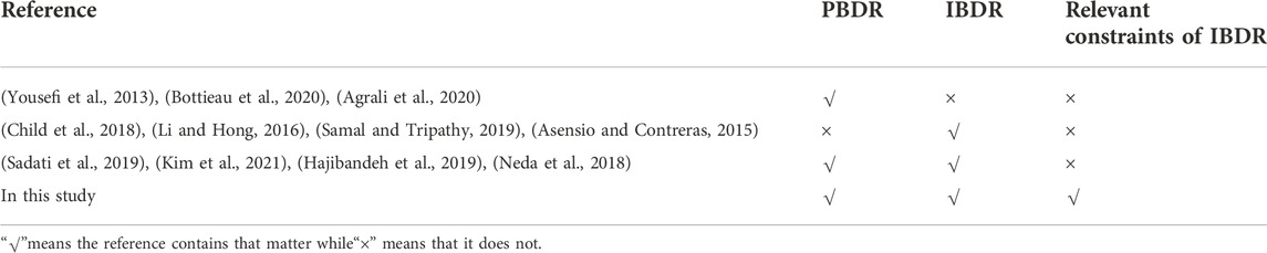
TABLE 1. Summary of previous studies considering DR.

In addition, some studies have explored the impact of energy storage systems (ESSs) on wind power consumption. A robust scheduling framework is proposed to obtain an optimal unit commitment in the system, which includes a large-capacity ESS, wind power, conventional units, and DR (Heydarian-Forushani et al., 2015). Arteaga and Zareipour (2019) established a model of ESS participating in the electricity market and studies the potential profit of ESS in providing multiple services. Khaloie et al. (2020) presented multistage electricity market trading strategies, taking environmental factors, ESS, thermal units, and wind power into account. According to the policy of promoting wind power development (Guangdong Provincial People’s Government, 2021), to ensure effective wind power consumption, encouraging the installation of energy storage systems for wind power generation is required. At present, few studies have analyzed the effects and economic benefits of energy capacity and power rating of ESS for wind power consumption.

Much literature has studied the supply–demand balance in power systems containing renewable energy using energy management. Ahmad et al. (2020a) presented the joint energy management and energy trading models, which provides low-cost electricity consumption to the distribution system. Ahmad et al. (2020b) proposed a demand side management (DSM) model to reduce electricity costs and minimize distribution losses. A heuristic algorithm is proposed by Ahmad et al. (2018) to develop an autonomous system, which can manage photovoltaic panels and wind turbines effectively and efficiently. Different DSM schemes are employed for consumer demand management by Yaqub et al. (2016) to optimize energy consumption with minimum consumer interaction. Ahmad et al. (2019) proposed a novel residential energy management approach for efficient energy consumption. Different from the abovementioned studies, mainly making use of active load resources through the DSM method, our research uses price signals (PBDR) and DR trading (IBDR) to assist supply–demand balance.

In this paper, a detailed DR model is established in the electricity market with large-scale wind power integration. Market trading includes two stages: day-ahead (DA) market and real-time (RT) market. DR includes PBDR and IBDR, of which IBDR is further divided into load shifting (LS) and load curtailment (LC). Different types of DR enable active consumers to play a flexible role in a two-stage electricity market. The main contributions of this study can be summarized as follows:

1) A detailed DR model is established, including PBDR and IBDR. The IBDR model not only contains its bidding and market clearing but also contains relevant constraints: maximum/minimum duration time, shifting/curtailment gap time, and shifting/curtailment frequency.

2) The effects of ESS energy capacity and power rating are investigated.

3) The influence of different wind power scales on system operation is analyzed.

4) The effects and economic benefits of different market participants for wind power consumption are analyzed.

2 Electricity market transaction mechanism

2.1 Market participants

DA market participants include conventional units (CUs), rapid adjustment units (RAUs), wind power, and LS, whereas RT market participants include RAUs, wind power, ESS, and LC.

2.2 Market transaction process

Considering PBDR, the system load will change in response to PBDR, followed by DA market and RT market transactions. The market transaction process is shown in Figure 1. The DA market is to clear 1 day in advance of the operation day to obtain the relevant resources operating status of the operation day. RT market transactions are conducted 15 min before the actual operation of the system, and rolling clearing is carried out to obtain the scheduling resource operating condition for the next 15 min.

FIGURE 1

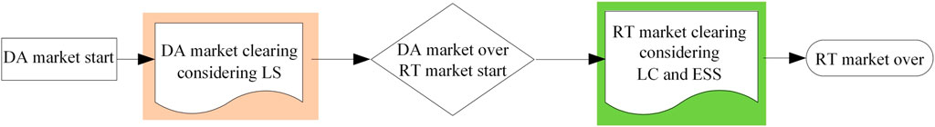
FIGURE 1. Market transaction process.

Consumers usually participate in PBDR based on price signals and do not directly participate in market transactions. LS only participates in the DA market to reduce the system peak–valley difference and ramping need for units. LC and ESS only participate in the RT market to reduce wind curtailment and load shedding. CUs have a slow adjustment speed, while RAUs have a rapid adjustment speed; therefore, CUs only participate in the DA market and RAUs participate in both DA and RT markets.

2.3 Market expense settlement

After the operation day, the relevant market participants will be charged through the DA and RT clearing electricity prices.

PBDR does not need to be settled. LS is settled according to the load shifting quantity and the DA price obtained from DA market clearing, while LC and ESS are settled by the RT price.

CUs are settled by the DA price and their power quantity, which is obtained by DA market clearing. When the RT market clearing power quantity of RAUs is greater than or equal to the DA market, the DA power quantity is settled by the DA price, and the excess part is settled by the RT price. On the contrary, when the clearing power quantity of RAUs in the RT market is less than the DA market, the RT power quantity will be settled by the DA price. The reduced power quantity will be subsidized to RAUs by the difference between DA price and RT price. It means that RAUs make room for wind power generation to utilize excess wind power in the RT market.

Like the RAUs, when the output of wind farms in the RT market is greater than the DA market, wind farms are settled by the DA price, and the excess part is settled by the RT price. On the contrary, when the output of wind power in the RT market is less than the DA market, the wind power is settled by the DA price. It means that the RT output of wind farms is less than the DA output, the wind power is insufficient, and the insufficient output is punished by the penalty coefficient.

3 Model introduction

3.1 Price-based demand response

The time-of-use (TOU) price is used to divide the peak–valley–flat periods of electricity consumption. The price signal is used to guide the consumers to change the power curve. The formula of PBDR is as follows:

$D_{n,t}=D_{n,t}^0\left\{1+{\displaystyle \sum }_{t^{\prime }=1}^T{E}_{t,t^{\prime }}\frac{\left({\rho }_{t^{\prime }}-{\rho }_{t^{\prime }}^0\right)}{{\rho }_{t^{\prime }}^0}\right\}(1)$

where $D_{n,t}$ and $D_{n,t}^0$, respectively, represent the load power demand before and after PBDR, ${\rho }_{t^{\prime }}^0$ and ${\rho }_{t^{\prime }}$ are, respectively, the electricity prices before and after PBDR in time $t^{\prime }$, and the prices are parameters set in advance. It relies on price difference to adjust consumers’ power consumption. $E_{t,t^{\prime }}$ is the elasticity coefficient of power demand between time t and $t^{\prime }$. Before PBDR, the electricity price for a whole day is the same; after PBDR, TOU prices are set up, and a day is divided into peak–valley–flat periods with different prices. The aforementioned formula embodies “self-elasticity” and “mutual -elasticity” of the consumer. The “self-elasticity” means that if ${\rho }_{t^{\prime }}>{\rho }_{t^{\prime }}^0$, the load power demand of period $t^{\prime }$ will decrease, while if ${\rho }_{t^{\prime }}<{\rho }_{t^{\prime }}^0$, it will increase. The “mutual-elasticity” means that if ${\rho }_{t^{\prime }}>{\rho }_{t^{\prime }}^0$, the load power demand of period t ($t\ne t^{\prime }$) will increase, while if ${\rho }_{t^{\prime }}<{\rho }_{t^{\prime }}^0$, it will decrease. Cutting the peak and filling the valley of the power curve can be realized by the consumers participating in PBDR. It is worth mentioning that PBDR is for all consumers, and its power changes have uncertainty; the analysis of PBDR uncertainty is beyond the scope of this study.

3.2 Incentive-based demand response

The IBDR discussed in this study can be divided into two types: LS and LC. Both types need to declare the shifting/curtailment quantity and price to the system operator. The declared quantity and price have a piecewise linear curve as shown in Figure 2, which shows a stepwise rise. The higher the compensation, the greater the LS/LC shift/curtail. According to Li and Hong (2016) and Neda et al. (2018), the bidding in this study is divided into four segments.

FIGURE 2

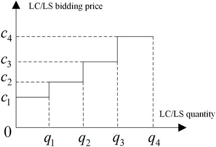
FIGURE 2. Demand response bidding curve.

3.2.1 Load shifting

LS participates in the DA market. Figure 3 shows the schematic of load shifting. The green parts represent load shifting, while the blue parts represent load recovery.

FIGURE 3

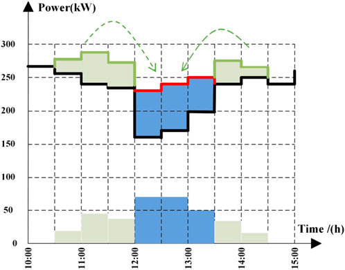
FIGURE 3. Schematic of load shifting.

The total load shifting quantity and its constraint are:

$P_{ls,t}^{LS}=q_{ls,0}^{LS}{u}_{ls,t}^{LS}+{\displaystyle \sum }_{m=1}^4{q}_{ls,m,t}^{LS}(2)$

$0\le q_{ls,m,t}^{LS}\le q_{ls,m,t}^{LS\max }{u}_{ls,t}^{LS}(3)$

where $P_{ls,t}^{LS}$ is the total load shifting quantity of DR aggregator ls in time t, $q_{ls,0}^{LS}$ is the initial minimum shifting quantity, $u_{ls,t}^{LS}$ is the binary status indicator of DR aggregator ls in time t, $q_{ls,m,t}^{LS}$ is the subsequent segmental load shifting, and $q_{ls,m,t}^{LS\max }$ is the segmental maximum load shifting.

The total cost of load shifting is:

$C_{ls,t}^{LS}=c_{ls,0,t}^{LS}{u}_{ls,t}^{LS}+{\displaystyle \sum }_{m=1}^4{c}_{ls,m,t}^{LS}{q}_{ls,m,t}^{LS}(4)$

where $C_{ls,t}^{LS}$ is the total cost and $c_{ls,0,t}^{LS}$ and $c_{ls,m,t}^{LS}$ are the offering prices of initial shifting quantity and the subsequent segmental shifting quantity, respectively.

$u_{ls,t}^{LS}=0,t\notin T_{ls}^{LS}(5)$

${\displaystyle \sum }_{t^{\prime }=t}^{t+LS{T}_{ls}^{\min }-1}{u}_{ls,t^{\prime }}^{LS}\ge LS{T}_{ls}^{\min }\left(u_{ls,t}^{LS}-u_{ls,t-1}^{LS}\right)(6)$

${\displaystyle \sum }_{t^{\prime }=t}^{t+LS{T}_{ls}^{\max }}{u}_{ls,t^{\prime }}^{LS}\le LS{T}_{ls}^{\max }(7)$

${\displaystyle \sum }_{t^{\prime }=t}^{t+LSga{p}_d-1}\left(1-u_{ls,t^{\prime }}^{LS}\right)\ge LSga{p}_{ls}\left(u_{ls,t-1}^{LS}-u_{ls,t}^{LS}\right)(8)$

Eq. 5 is the constraint of shifting time, Eqs. 6–7 are the maximum/minimum duration shifting time limit, and Eq. 8 is the constraint of load shifting time interval. $T_{ls}^{LS}$ is the period allowing to shift, $LS{T}_{ls}^{\max }$/$LS{T}_{ls}^{\min }$ is the maximum/minimum duration shifting time, and $LSga{p}_{ls}$ is the minimum time interval.

The constraints of load shifting times are:

${\varsigma }_{ls,t}^{LS}=\max \left\{0u_{ls,t}^{LS}-u_{ls,t-1}^{LS}\right\}(9)$

${\displaystyle \sum }_{t\in T}{\xi }_{ls,t}^{LS}\le M_{ls}^{LS}(10)$

where ${\varsigma }_{ls,t}^{LS}$ is an auxiliary variable used to record the shifting times within the scheduling periods and $M_{ls}^{LS}$ is the maximum transfer time of DR aggregator ls.

The constraints of power recovery quantity and recovery time are:

${\displaystyle \sum }_{t\in T_{ls}^{LR}}{P}_{ls,t}^{LR}={\displaystyle \sum }_{t\in T_{ls}^{LS}}{\lambda }_{ls}{P}_{ls,t}^{LS}(11)$

$u_{ls,t}^{LR}{P}_{ls}^{LR\min }\le P_{ls,t}^{LR}\le u_{ls,t}^{LR}{P}_{ls}^{LR\max },\forall t\in T_{ls}^{LR}(12)$

$u_{ls,t}^{LR}=0,\forall t\notin T_{ls}^{LR}(13)$

where $P_{ls,t}^{LR}$ is the recovery quantity, ${\lambda }_{ls}$ is the recovery coefficient; $u_{ls,t}^{LR}$ is a binary status indicator of power recovery in time t, $P_{ls}^{LR\max }$ and $P_{ls}^{LR\min }$ are the upper and lower limits of recovery power in each t, respectively, and $T_{ls}^{LR}$ is the recoverable time period.

3.2.2 Load curtailment

LC participates in the RT market. Figure 4 shows the schematic of load curtailment; the blue parts represent the load curtailment. The total load curtailment quantity and its curtailment quantity are:

$P_{lc,t}^{LC}=q_{lc,0,t}^{LC}{u}_{lc,t}^{LC}+{\displaystyle \sum }_{m=1}^4{q}_{lc,m,t}^{LC}(14)$

$0\le q_{lc,m,t}^{LC}\le q_{lc,m,t}^{\max }{u}_{lc,t}^{LC}(15)$

where $P_{lc,t}^{LC}$ is the total load curtailment quantity of DR aggregator lc in time t, $q_{lc,0}^{LC}$ is the initial minimum curtailment quantity, $u_{lc,t}^{LC}$ is the binary status indicator of DR aggregator lc in time t, $q_{lc,m,t}^{LC}$ is the subsequent segmental load curtailment, and $q_{lc,m,t}^{LC\max }$ is the segmental maximum curtailment load.

FIGURE 4

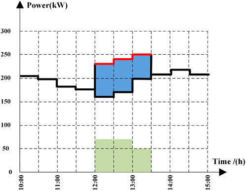
FIGURE 4. Schematic of load curtailment.

The total cost of load curtailment is:

$C_{lc,t}^{LC}=c_{lc,0,t}^{LC}{u}_{lc,t}^{LC}+{\displaystyle \sum }_{m=1}^4{c}_{lc,m,t}^{LC}{q}_{lc,m,t}^{LC}(16)$

where $C_{lc,t}^{LC}$ is the total cost $c_{lc,0,t}^{LC}$ and $c_{lc,m,t}^{LC}$ are the offering price of the initial curtailment quantity and the subsequent segmental curtailment quantity, respectively.

$u_{lc,t}^{LC}=0,t\notin T_{lc}^{LC}(17)$

${\displaystyle \sum }_{t^{\prime }=t}^{t+LC{T}_{lc}^{\min }-1}{u}_{lc,t^{\prime }}^{LC}\ge LC{T}_{lc}^{\min }\left(u_{lc,t}^{LC}-u_{lc,t-1}^{LC}\right)(18)$

${\displaystyle \sum }_{t^{\prime }=t}^{t+LC{T}_{lc}^{\max }}{u}_{lc,t^{\prime }}^{LC}\le LC{T}_{lc}^{\max }(19)$

${\displaystyle \sum }_{t^{\prime }=t}^{t+LCga{p}_d-1}\left(1-u_{lc,t^{\prime }}^{LC}\right)\ge LCga{p}_{lc}\left(u_{lc,t-1}^{LC}-u_{lc,t}^{LC}\right)(20)$

Eq. 17 is the constraint of curtailable time, Eqs. 18–19 are the maximum/minimum duration curtailment time limits, and Eq. 20 is the constraint of load curtailment time interval. $T_{lc}^{LC}$ is the period allowing to curtail, $LC{T}_{lc}^{\max }$ and $LC{T}_{lc}^{\min }$ are the maximum and minimum duration curtailment time, respectively, and $LCga{p}_{lc}$is the minimum time interval.

The constraints of load curtailment times are:

${\varsigma }_{lc,t}^{LC}=\max \left\{0,u_{lc,t}^{LC}-u_{lc,t-1}^{LC}\right\}(21)$

${\displaystyle \sum }_{t\in T}{\xi }_{lc,t}^{LC}\le M_{lc}^{LC}(22)$

where ${\varsigma }_{lc,t}^{LC}$ is an auxiliary variable used to record the curtailment times within the scheduling period and $M_{lc}^{LC}$ is the maximum curtailment times of DR aggregator lc.

3.3 Day-ahead market clearing model

The objective function of the DA market is to minimize the total cost:

$\min \mathit{Cos}{t}^{DA}={\displaystyle \sum }_{t=1}^T\left\{\begin{array}{l}{\displaystyle \sum }_{i=1}^{NG}\left[\begin{array}{l}{C}_{i,t}\left(P_{i,t}\right)+S{U}_{i,t}\\ +S{D}_{i,t}\end{array}\right]+{\displaystyle \sum }_{if=1}^{N{G}_f}\left[\begin{array}{l}{C}_{if,t}^{DA}\left(P_{if,t}^{DA}\right)+S{U}_{if,t}\\ +S{D}_{if,t}\end{array}\right]+{\displaystyle \sum }_{ls}^{NLS}{C}_{l\mathrm{s},t}^{LS}+\\ M_1{\displaystyle \sum }_{w=1}^{NW}Qwin{d}_{w,t}^{DA}+{\displaystyle \sum }_{l=1}^{NL}{M}_2\left[S{L}_{l,t}^{DA+}+S{L}_{l,t}^{DA-}\right]\end{array}\right\}(23)$

where $C_{i,t}\left(P_{i,t}\right),S{U}_{i,t},S{D}_{i,t}$ is the generation cost and start-up/shutdown cost of CUs i; $C_{if,t}^{DA}\left(P_{if,t}^{DA}\right),S{U}_{if,t},S{D}_{if,t}$ is the generation cost and start-up/shutdown cost of RAUs if; $C_{l\mathrm{s},t}^{LS}$ is the cost of LS, and the LS model is described in detail in Section 3.2.1; $M_1$ and $M_2$ are the wind power curtailment penalty coefficient and the network power flow constraint penalty coefficient, respectively; $Qwin{d}_{w,t}^{DA}$ is wind power curtailment in the DA market; and $S{L}_{l,t}^{DA+}$ and $S{L}_{l,t}^{DA-}$ are slack variables for forward and reverse power flow of line l in the DA market, respectively. The decision variables are $u_{i,t},u_{if,t},u_{ls,t}^{LS},P_{i,t},P_{if,t}^{DA},q_{ls,m,t}^{LS},Qwin{d}_{w,t}^{DA}$ subject to the following constraints. The meaning of the symbols can be obtained from the nomenclature table.

3.3.1 Day-ahead system power balance constraints

$\{\begin{array}{l}{\displaystyle \sum }_{i=1}^{NG}{P}_{i,t}+{\displaystyle \sum }_{if=1}^{N{G}_f}{P}_{if,t}^{DA}+{\displaystyle \sum }_{w=1}^{NW}{P}_{w,t}^{DA}={\displaystyle \sum }_{n=1}^N{D}_{n,t}+{\displaystyle \sum }_{ls=1}^{NLS}\left(P_{ls,t}^{LR}-P_{ls,t}^{LS}\right)\\ P_{w,t}^{DA}=P_{w,t}^{DA\max }-Qwin{d}_{w,t}^{DA}\end{array}(24)$

where $P_{i,t}$ is the power generation of CUs, $P_{if,t}^{DA}$ is the power generation of RAUs, $P_{w,t}^{DA}$ is DA wind power consumption, $P_{w,t}^{DA\max }$ is the maximum wind power that is predicted in DA, and $D_{n,t}$ is the load power demand at bus n after PBDR.

3.3.2 System power flow constraints

$\{\begin{array}{l}{P}^{SP}=B\theta \\ P_{j,k}=\left({\theta }_j-{\theta }_k\right)/x_{jk}\\ P_{j,k}-S{L}_{l,t}^{DA+}\le P_{j,k}^{\max }\\ P_{j,k}+S{L}_{l,t}^{DA-}\ge -P_{j,k}^{\max }\\ j,k=\mathrm{1,2,3}\dots N\end{array}(25)$

where $P^{SP}$ is the N-dimensional column vector of injected power of bus n. The first and second rows of Eq. 25 represent the DC power flow, and the third and fourth rows represent the maximum forward and reverse flow of the branch between bus j and k, respectively.

3.3.3 Unit constraints

The related constraints of CUs and RAUs are similar, which include power generation upper and lower limit, ramp up/down limit, and minimum start-up/shutdown duration time limit. For brevity, only the CU model is presented here.

1) Constraints of power generation

$\{\begin{array}{l}0\le q_{i,t,m}\le u_{i,t}{q}_{i,m}^{\max }\\ P_{i,t}=u_{i,t}{q}_{i,0}+{\displaystyle \sum }_{m=1}^4{q}_{i,m,t}\\ C_{i,t}\left(P_{i,t}\right)=c_{i,0}{u}_{i,t}+{\displaystyle \sum }_{m=1}^4{c}_{i,m,t}{q}_{i,m,t}\end{array}(26)$

where $q_{i,0}$ is the initial minimum power generation, $u_{i,t}$ is the binary status indicator of CU i in time t, $q_{i,t,m}$ is the subsequent segmental power generation, $q_{i,m}^{\max }$ is the segmental maximum power generation, and $c_{i,0}$ and $c_{i,m,t}$ are the offering price of initial power generation and the subsequent segmental power generation, respectively.

2) Constraints of ramp up/down

$\{\begin{array}{l}{P}_{i,t}-P_{i,t-1}\le R{U}_i{u}_{i,t-1}+SU{R}_i{y}_{i,t}\\ P_{i,t-1}-P_{i,t}\le R{D}_i{u}_{i,t}+SD{R}_i{z}_{i,t}\end{array}(27)$

where $R{U}_i$($R{D}_i$) is the ramp-up (ramp-down) rate of CU I, $SU{R}_i$($SD{R}_i$) is the startup (shutdown) ramp rate of CU i, and $y_{i,t}$($z_{i,t}$) is the startup (shutdown) binary status indicator of CU i in time t.

3) Constraints of minimum start-up/shutdown duration time

$\{\begin{array}{l}{u}_{i,t}=1,t\in \left[1,U_i\right]\\ {\displaystyle \sum }_{x=t}^{t+T_{oni}-1}{u}_{i,x}\ge T_{oni}\left(u_{i,t}-u_{i,t-1}\right),t\in \left[U_i+1,T-T_{oni}+1\right]\\ {\displaystyle \sum }_{x=t}^T{u}_{i,x}\ge \left(u_{i,t}-u_{i,t-1}\right),t\in \left[T-T_{oni}+2,T\right]\end{array}(28)$

$\{\begin{array}{l}{u}_{i,t}=0,t\in \left[1,D_i\right]\\ {\displaystyle \sum }_{x=t}^{t+T_{offi}-1}\left(1-u_{i,x}\right)\ge T_{offi}\left(u_{i,t-1}-u_{i,t}\right),t\in \left[D_i+1,T-T_{offi}+1\right]\\ {\displaystyle \sum }_{x=t}^T{u}_{i,x}\ge \left(u_{i,t-1}-u_{i,t}\right),t\in \left[T-T_{offi}+2,T\right]\end{array}(29)$

where $U_i$($D_i$) represents the period during which CU i must be on/off at the beginning of the scheduling cycle; it is determined by the state of CU i at the end of the last scheduling cycle. $T_{oni}$($T_{offi}$) is the period of the minimum on/off time of CU i.

The relevant constraints of LS are given in Eqs. 2–13.

3.4 Real-time market clearing model

RT market transactions are conducted 15 min before the actual operation of the system, and rolling clearing is carried out to obtain the scheduling resource operating condition for the next 15 min.

$\min \mathit{Cos}{t}^{RT}=\left\{\begin{array}{l}{\displaystyle \sum }_{if=1}^{N{G}_f}{C}_{if,t}^{RT}\left(P_{if,t}^{RT}\right)+{\displaystyle \sum }_{lc=1}^{NLC}{C}_{lc,t}^{LC}+{\displaystyle \sum }_{ib=1}^{NB}{C}_{ib,t}^{degra}+M_1{\displaystyle \sum }_{n=1}^{N}Qloa{d}_{n,t}^{RT}+{\displaystyle \sum }_{l=1}^{NL}{M}_2\left[S{L}_{l,t}^{RT+}+S{L}_{l,t}^{RT-}\right]\\ +M_3{\displaystyle \sum }_{w=1}^{N_W}Qwin{d}_{w,t}^{RT},t=\mathrm{1,2,3},...,T\end{array}\right\}(30)$

where $C_{if,t}^{RT}\left(P_{if,t}^{RT}\right)$ is the generation cost of RAU if in the RT market, $C_{lc,t}^{LC}$ is the cost of load curtailment; the LC model is described in detail in Section 3.2.2, $C_{ib,t}^{degra}$ is the degradation cost of ESS, $Qwin{d}_{w,t}^{RT}$,$Qloa{d}_{n,t}^{RT}$ are the wind power curtailment and load shedding in the RT market, respectively, $M_1$,$M_2$,$M_3$ are penalty coefficients; and $S{L}_{l,t}^{RT+},S{L}_{l,t}^{RT-}$ are slack variables for forward and reverse power flow of line l in the RT market, respectively. The decision variables are $u_{lc,t}^{LC},u_{ib,t}^{ch},u_{ib,t}^{dis}{P}_{if,t}^{RT},q_{lc,m,t}^{LC},$ $P_{ib,t}^{ch},P_{ib,t}^{dis},Qwin{d}_{w,t}^{RT},Qloa{d}_{n,t}^{RT}$, subject to following constraints. The meaning of the symbols can be obtained from the nomenclature table.

3.4.1 Real-time system power balance constraints

$\{\begin{array}{l}{\displaystyle \sum }_{i=1}^{NG}{P}_{i,t}+{\displaystyle \sum }_{if=1}^{N{G}_f}{P}_{if,t}^{RT}+{\displaystyle \sum }_{w=1}^{NW}{P}_{w,t}^{RT}+{\displaystyle \sum }_{ib=1}^{NB}\left(P_{ib,t}^{dis}-P_{ib,t}^{ch}\right)={\displaystyle \sum }_{n=1}^N(D_{n,t}^{LS}-Qloa{d}_{n,t}^{RT})-{\displaystyle \sum }_{lc=1}^{NLC}{P}_{lc,t}^{LC}\\ P_{w,t}^{RT}=P_{w,t}^{RT\max }-Qwin{d}_{w,t}^{RT}\end{array}(31)$

where $P_{i,t}$ is the power generation of CUs, which is given by the DA market clearing results, $P_{if,t}^{RT}$ is the power generation of RAUs in the RT market, $P_{w,t}^{RT}$ is the RT wind power consumption, $P_{w,t}^{RT\max }$ is the maximum wind power, which is predicted in RT, $P_{ib,t}^{dis}$ and $P_{ib,t}^{ch}$ are the discharge and charge power of ESS, respectively, and $D_{n,t}^{LS}$ is the load power demand at bus n after LS.

3.4.2 Energy storage system constraints

$\{\begin{array}{l}0\le P_{ib,t}^{ch}\le P_{ib,t}^{ch\max }{u}_{ib,t}^{ch}\\ 0\le P_{ib,t}^{dis}\le P_{ib,t}^{dis\max }{u}_{ib,t}^{dis}\end{array}(32)$

$\{\begin{array}{l}E{L}_{ib,t}=E{L}_{ib,t-1}+∆\mathrm{t}\left({\eta }_{ch}{P}_{ib,t-1}^{ch}-\left(P_{ib,t-1}^{ch}/{\eta }_{dis}\right)\right)\\ E{L}_{ib,t}\le E{L}_{ib}^{\max }\end{array}(33)$

$C_{ib,t}^{degra}={\lambda }_{ib}\left(P_{ib,t}^{ch}+P_{ib,t}^{dis}\right)(34)$

$u_{ib,t}^{dis}+u_{ib,t}^{ch}\le 1(35)$

where $P_{ib,t}^{dis\max }$ and $P_{ib,t}^{ch\max }$ are the maximum discharge and charge power, respectively, $u_{ib,t}^{dis}$ and $u_{ib,t}^{ch}$ are binary status indicators ESS, $E{L}_{ib,t}$ is the stored power energy of ESS in time t; $E{L}_{ib,t}^{\max }$ is the stored power energy of ESS, ${\eta }_{ch}$ and ${\eta }_{dis}$ are charge and discharge efficiency coefficients, respectively, and ${\lambda }_{ib}$ is the ESS degradation coefficient.

For the relevant constraints of LC, refer to Eqs. 14–22, and for the other constraints (power generation upper and lower limit for RAUs and ramp up/down limit for RAUs), refer to the day-ahead market model.

4 Results and discussions

In this section, the numerical results are presented to validate the effectiveness of the proposed model. Case studies, carried out in the IEEE 30 bus system, are shown in Figure 5. The IEEE-30 bus system is a typical power grid, and the studies in a typical power system can verify the accuracy and effectiveness of the proposed models. There are three conventional units, one rapid adjustment unit, four wind farms, and four IBDR aggregators. A day is divided into 96 periods. PBDR parameters such as peak–valley–flat periods division and corresponding electricity price are shown in Table 2. The self-elasticity coefficient and mutual-elasticity coefficient are set as -0.12 and 0.012, respectively (Aalami et al., 2010). There are four IBDR aggregators in the bus, 5, 7, 21, and 30, where the power demand is large. The total aggregated load of aggregators accounts for 7% of the total system load. The predictive DA and RT wind power are shown in Figure 6. The proportion of wind power to the total load of the system is 50%. The real wind power historical data of Belgium in Elia are scaled down and used as the wind power DA forecast output and RT forecast output in this study. In DA market clearing and RT market clearing, the objective of wind power is to reduce the amount of wind curtailment as much as possible, and the wind power consumption does not exceed the predicted output.

FIGURE 5

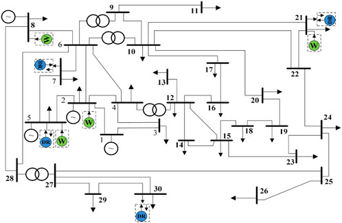
FIGURE 5. IEEE 30 bus system.

TABLE 2

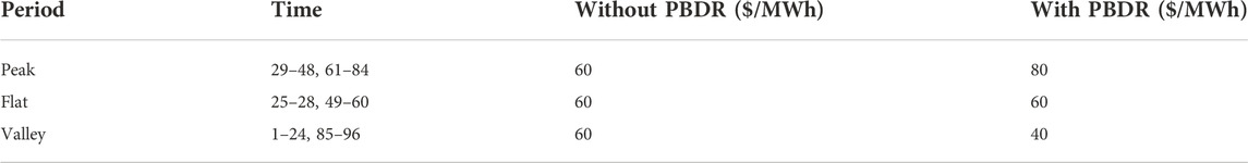
TABLE 2. TOU electricity price for PBDR.

FIGURE 6

FIGURE 6. Day-ahead and real-time wind power.

The DA and RT two-stage market clearing model are MILP problems essentially, which can be efficiently solved by GAMS using the CPLEX solver. The solution flowchart is shown in Figure 7.

FIGURE 7

FIGURE 7. Solution flowchart.

4.1 Day-ahead market and real-time market clearing results

Figure 8 shows the comparison between the original load of the system and the load considering PBDR and LS. After PBDR and LS, the load decreases in the peak periods (29–48 and 61–84) and increases in the valley periods (1–24 and 85–96), making the peak–valley difference of the load curve smaller. It can enhance the reliability and security of system operation.

FIGURE 8

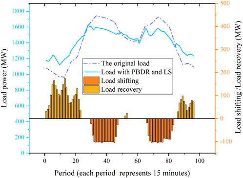
FIGURE 8. Original load and load with PBDR and LS.

Figure 9 shows the curtailment of LC in the RT market. Load curtailment takes place during the peak demand periods (29–48, 61–84). Figure 10 shows one of the ESS’s charge power, discharge power, and stored energy. ESS discharges when the RT wind power is lower than DA and charges when the RT wind power is higher. LC and ESS are used to solve the uncertainty problem of wind power. Each wind farm is equipped with ESS. ESS does not participate in bidding in the RT market directly, and the charge/discharge power are obtained by solving the RT model.

FIGURE 9

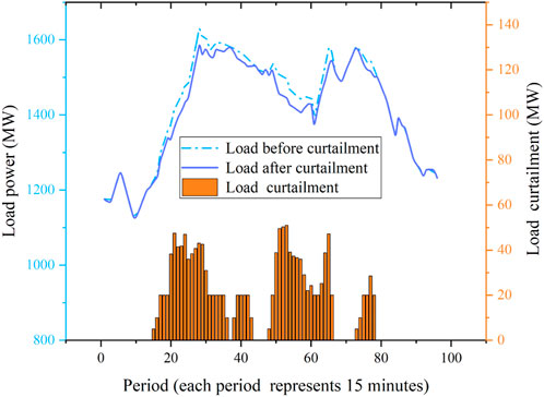
FIGURE 9. Load curtailment in the RT market.

FIGURE 10

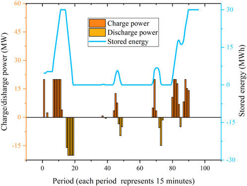
FIGURE 10. ESS’s charge power, discharge power, and stored energy.

4.2 Effects of incentive-based demand response relevant constraints and different incentive-based demand response scales

The IBDR model in this study not only includes its bidding and market clearing but also contains relevant constraints: maximum/minimum duration time, shifting/curtailment gap time, and shifting/curtailment frequency. The IBDR model does not contain these constraints in many reports in the literature. The effects of IBDR relevant constraints are analyzed in this section, and the results are shown in Table 3. Without relevant constraints, the maximum duration time and shifting/curtailment frequency are 28 and 3, respectively, which are not adjustable. With relevant constraints, the maximum duration time and shifting/curtailment frequency are 16 and 2, respectively, which are adjustable. There is a limit on load shifting or load curtailment; too long duration time and too high frequency for IBDR will have a great impact on the production and life of IBDR providers. Therefore, relevant constraints are considered for the IBDR model in this study.

TABLE 3

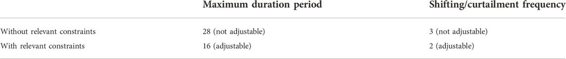
TABLE 3. Effects of IBDR with or without relevant constraints.

To obtain the best scales of DR, we analyzed the effects of different DR scales. The results are shown in Table 4. The proportion of DR in the total system load increased from 1 to 10%. When the DR scale increases, system cost, wind power curtailment, and the system total ramping need (including ramp up/down) of the unit show a decreasing trend. However, the marginal benefit brought by the DR per scale is constantly decreasing. When the proportion of DR increases to 7%, the system cost and wind power curtailment no longer decrease significantly. Therefore, in the following studies, the DR scale is set at 7%.

TABLE 4

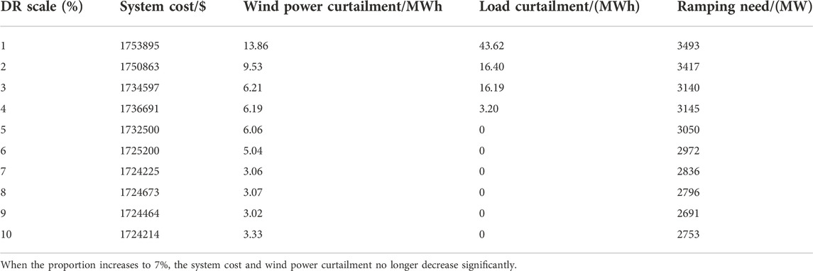
TABLE 4. Effects of different DR scales.

4.3 Effects of energy storage system energy capacity and power rating

The effects of ESS energy capacity and power rating are investigated. Figure 11 and Figure 12 respectively show the system cost and wind power curtailment under different energy capacities and power ratings. When energy capacity and power rating are improved, the total system cost and wind power curtailment can be reduced effectively. This is because the ESS with a large capacity and large charge, discharge power rating can store more excess wind power, making full use of wind energy, and reducing the generation cost of units. It is worth noting that due to the investment cost and operation maintenance cost of the ESS, when the energy capacity and power rating are too large, the total system cost will increase. When the energy capacity/power rating is 50 MWh/25MW, the cost of the system is higher than when it is 30 MWh/15 MW.

FIGURE 11

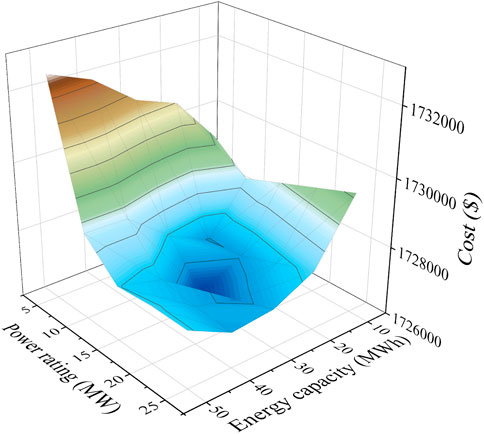
FIGURE 11. System cost.

FIGURE 12

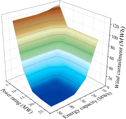
FIGURE 12. Wind power curtailment.

The system cost and wind curtailment at the lowest power rating and maximum capacity (50 MWh/5 MW) are larger than the highest power rating and minimum capacity (10 MWh/25 MW), respectively. Although these two conditions are not the most conducive to wind power consumption, the combination of high capacity and low power rating negatively affects wind consumption more. Therefore, if the budget of the ESS is limited during the system planning, a relatively high power rating should be given priority. The same conclusion can also be drawn from the variation trend in Figure 11 and Figure 12. As the power rating increases from small to large, the reduction trend of the system cost and wind power curtailment becomes more intense than the capacity increases.

4.4 Effects of wind power scale

The effects of the wind power scale were analyzed, and the proportion of wind power in the total load changed from 10 to 70%. The results are shown in Table 5. With the increasing proportion of wind power, the system cost is constantly decreasing, and the ramp need of unit is increasing. When the proportion of wind power is 70%, the wind curtailment is 323 MWh, which is 1.4% of total wind power, indicating that it is difficult for the system to utilize such a high proportion of wind power completely. However, the proportion of wind curtailment is acceptable.

TABLE 5

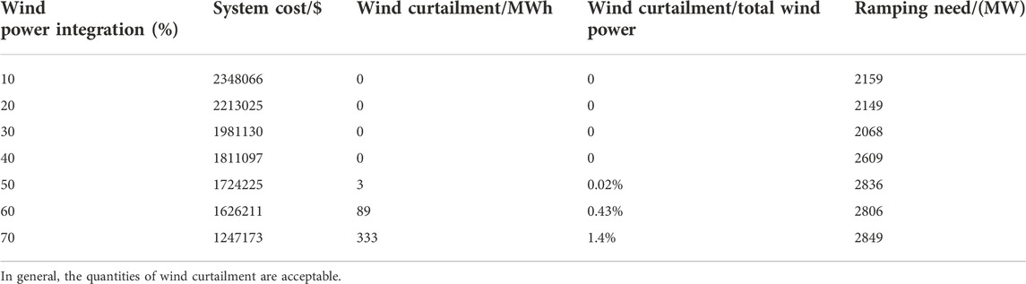
TABLE 5. Effects of different wind power integrations.

Figure 13 shows the DA and RT market clearing price and the variation of the total load shifting and load curtailment within a day. With the increasing wind power, the average DA and RT price reduces. The DA price reduces from $60 to $30, and the RT price reduces from $50 to $20. RT price is lower than DA price because when wind curtailment appears in some periods, there will be some negative electricity, and it is more likely to appear in the RT market. Therefore, the RT price will be lower. The total load curtailment decreases (from 900 to 300 MWh) with the increasing wind power output because when the proportion of wind power is small, the power generation of CUs and RAUs is large, the market clearing price will be high, and LC will curtail more load. With the increasing wind power, the power generation of CUs and RAUs gradually reduces, the system clearing price decreases, and LC will curtail less load. Compared with the load curtailment, the overall trend of the load shifting does not change much with the increase of the wind power output.

FIGURE 13

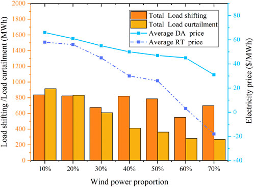
FIGURE 13. Market clearing price, total load shifting, and load curtailment.

4.5 Effects of different market participants

The effects of different market participants are analyzed. The market participants in various cases are shown in Table 6.

TABLE 6

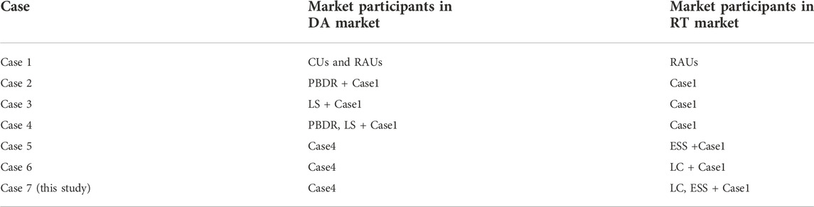
TABLE 6. Different cases of market participants.

Figure 14 shows the comparison of PBDR and LS in cases 1–4, and Table 7 shows the related results in each case. According to cases 1–4 in Figure 14 and Table 7, both PBDR and LS can reduce the load in peak periods (29–48 and 61–84) and increase the load in valley periods (1–24 and 85–96). It can help to reduce the peak–valley difference of the system, the ramping need of units, and the system cost. Considering LS alone is more effective than considering PBDR alone; the combination of PBDR and LS works best.

FIGURE 14

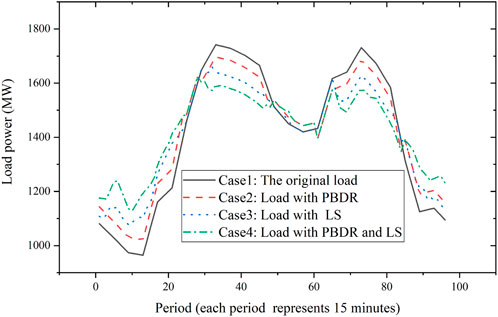
FIGURE 14. Comparison of PBDR and LS.

TABLE 7

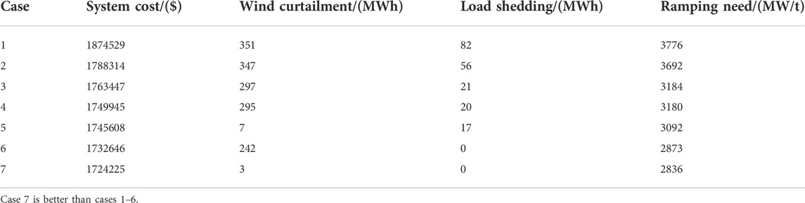
TABLE 7. Comparison of different cases.

Figure 15 shows the comparison of wind curtailment and load shedding in each case. There are large wind curtailments in cases 1–4; this means that cases 1–4 cannot utilize wind power efficiently. Cases 1–4 show load shedding which is unacceptable. Case 5 curtails little wind power and shows load shedding. Case 6 shows wind curtailment but does not cause load shedding. Case 7 does not curtail wind power and does not show load shedding. According to the previous analysis, ESS can effectively avoid wind curtailment, but each ESS has a charge power and discharge power limit. When the RT wind power is much smaller than the DA wind power, a serious shortage of the system supply will appear. The system supply shortage will not be solved just by relying on the RAUs and ESS, which will cause load shedding. LC provides additional regulation capacity to the system, which makes the system appear less or no load shedding and enhances the reliability of the system’s power supply to consumers. The combination of ESS and LC works best.

FIGURE 15

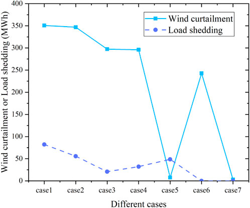
FIGURE 15. Wind curtailment and load shedding.

Case 7, the method adopted in this study, is better than cases 1–6 in terms of system cost, wind curtailment, load shedding, and ramping need.

5 Conclusion

Large-scale wind power integration has brought great challenges to the balance of supply and demand in the power system. DR and ESS play crucial roles in the consumption of large-scale wind power. This study designs a DA and RT two-stage electricity market trading method including various market participants: wind power, ESS, and multiple types of DR. An innovative DR model is established considering PBDR and IBDR. The IBDR model not only includes its bidding and market clearing but also contains relevant constraints: maximum/minimum duration time, shifting/curtailment gap time, and shifting/curtailment frequency. Some examples are studied in the IEEE-30 bus system. The roles and economic effects of various market participants in the consumption of large-scale wind power are analyzed. The conclusions are as follows:

1) It makes more sense to take relevant constraints of IBDR into account than not. The optimal proportion of DR in this study is about 7%.

2) Increasing the energy capacity and power rating of ESS can effectively reduce the total system cost and system wind curtailment, and the power rating increase should be given priority.

3) It can achieve the best effect when PBDR and LS are considered in the DA market, while ESS and LC participate in the RT market. Minimum system cost, wind curtailment, and load shedding can be attained.

For future research, the uncertainty of DR can be considered, and relevant stochastic optimization techniques will be studied.

Data availability statement

The raw data supporting the conclusions of this article will be made available by the authors, without undue reservation.

Author contributions

All authors listed have made a substantial, direct, and intellectual contribution to the work and approved it for publication.

Funding

The authors thank the support of the Natural Science Foundation of Guangdong Province (No. 2021A1515012073) and the National Natural Science Foundation of China (No. 52077083).

Conflict of interest

The authors declare that the research was conducted in the absence of any commercial or financial relationships that could be construed as a potential conflict of interest.

Publisher’s note

All claims expressed in this article are solely those of the authors and do not necessarily represent those of their affiliated organizations, or those of the publisher, the editors, and the reviewers. Any product that may be evaluated in this article, or claim that may be made by its manufacturer, is not guaranteed or endorsed by the publisher.

References

Aalami, H. A., Moghaddam, M. P., and Yousefi, G. R. (2010). Demand response modeling considering Interruptible/Curtailable loads and capacity market programs. Appl. Energy 87 (1), 243–250. doi:10.1016/j.apenergy.2009.05.041

CrossRef Full Text | Google Scholar

Agrali, C., Gultekin, H., Tekin, S., and Oner, N. (2020). Measuring the value of energy storage systems in a power network. Int. J. Electr. Power & Energy Syst. 120, 106022. doi:10.1016/j.ijepes.2020.106022

CrossRef Full Text | Google Scholar

Ahmad, H., Ahmad, A., and Ahmad, S. (2018). “Efficient energy management in a microgrid[C],” in 2018 International Conference on Power Generation Systems and Renewable Energy Technologies (PGSRET), Pakistan, 10-12 Sept. 2018, 1–5.

Google Scholar

Ahmad, S., Naeem, M., and Ahmad, A. (2019). Low complexity approach for energy management in residential buildings. Int. Trans. Electr. Energy Syst. 29 (1), e2680. doi:10.1002/etep.2680

CrossRef Full Text | Google Scholar

Ahmad, S., Alhaisoni, M. M., Naeem, M., Ahmad, A., and Altaf, M. (2020). Joint energy management and energy trading in residential microgrid system. IEEE Access 8, 123334–123346. doi:10.1109/access.2020.3007154

CrossRef Full Text | Google Scholar

Ahmad, S., Naeem, M., and Ahmad, A. (2020). Unified optimization model for energy management in sustainable smart power systems. Int. Trans. Electr. Energy Syst. 30 (4), e12144. doi:10.1002/2050-7038.12144

CrossRef Full Text | Google Scholar

Arteaga, J., and Zareipour, H. (2019). A price-maker/price-taker model for the operation of battery storage systems in electricity markets. IEEE Trans. Smart Grid 10 (6), 6912–6920. doi:10.1109/tsg.2019.2913818

CrossRef Full Text | Google Scholar

Asensio, M., and Contreras, J. (2015). Risk-constrained optimal bidding strategy for pairing of wind and demand response resources[J]. IEEE Trans. Smart Grid 8, 1. doi:10.1109/TSG.2015.2425044

CrossRef Full Text | Google Scholar

Bottieau, J., Hubert, L., Grève, Z. D., Vallee, F., and Toubeau, J. F. (2020). Very-short-term probabilistic forecasting for a risk-aware participation in the single price imbalance settlement. IEEE Trans. Power Syst. 35 (2), 1218–1230. doi:10.1109/tpwrs.2019.2940756

CrossRef Full Text | Google Scholar

Child, M., Bogdanov, D., and Breyer, C. (2018). The role of storage technologies for the transition to a 100% renewable energy system in Europe[J]. Energy Procedia 155, 44. doi:10.1016/j.egypro.2018.11.067

CrossRef Full Text | Google Scholar

Guangdong Provincial People's Government (2021). The general office of the Guangdong provincial People's government issued the notice on promoting the orderly development of offshore wind power and the implementation plan for the sustainable development of related industries[J]. Bull. Guangdong Prov. People's Gov. 18 (17), 23–29. Available at: http://www.gd.gov.cn/zwgk/gongbao/2021/17/content/post_3367237.html.

Google Scholar

Hajibandeh, N., Ehsan, M., Soleymani, S., Shafie-khah, M., and Catalao, J. P. (2019). Prioritizing the effectiveness of a comprehensive set of demand response programs on wind power integration. Int. J. Electr. Power & Energy Syst. 107, 149–158. doi:10.1016/j.ijepes.2018.11.024

CrossRef Full Text | Google Scholar

Heydarian-Forushani, E., Golshan, M. E. H., Moghaddam, M. P., Shafie-khah, M., and Catalao, J. (2015). Robust scheduling of variable wind generation by coordination of bulk energy storages and demand response. Energy Convers. Manag. 106, 941–950. doi:10.1016/j.enconman.2015.09.074

CrossRef Full Text | Google Scholar

Jamali, A., Aghaei, J., Esmaili, M., Nikoobakht, A., Niknam, T., Shafie-khah, M., et al. (2020). Self-scheduling approach to coordinating wind power producers with energy storage and demand response. IEEE Trans. Sustain. Energy 11 (3), 1210–1219. doi:10.1109/tste.2019.2920884

CrossRef Full Text | Google Scholar

Khaloie, H., Abdollahi, A., Shafie-Khah, M., Siano, P., Catalao, J., Nojavan, S., et al. (2020). Coordinated wind-thermal-energy storage offering strategy in energy and spinning reserve markets using a multi-stage model[J]. Appl. Energy 259, 114168. doi:10.1016/j.apenergy.2019.114168

CrossRef Full Text | Google Scholar

Khaloie, H., Anvari-Moghaddam, A., Contreras, J., Toubeau, J. F., Siano, P., and Vallee, F. (2022). Offering and bidding for a wind producer paired with battery and CAES units considering battery degradation. Int. J. Electr. Power & Energy Syst. 136, 107685. doi:10.1016/j.ijepes.2021.107685

CrossRef Full Text | Google Scholar

Kim, H. J., Kim, M. K., and Lee, J. W. (2021). A two-stage stochastic p-robust optimal energy trading management in microgrid operation considering uncertainty with hybrid demand response. Int. J. Electr. Power & Energy Syst. 124, 106422. doi:10.1016/j.ijepes.2020.106422

CrossRef Full Text | Google Scholar

Le, L., Fang, J., Zhang, M., Zeng, K., Ai, X., Wu, Q., et al. (2021). Data-driven stochastic unit commitment considering commercial air conditioning aggregators to provide multi-function demand response. Int. J. Electr. Power & Energy Syst. 129 (1), 106790. doi:10.1016/j.ijepes.2021.106790

CrossRef Full Text | Google Scholar

Li, Y. C., and Hong, S. H. (2016). Real-time demand bidding for energy management in discrete manufacturing facilities[J]. IEEE Trans. Industrial Electron. 64 (1), 1. doi:10.1109/TIE.2016.2599479

CrossRef Full Text | Google Scholar

Neda, H., Miadreza, S. K., Saber, T., Shahab, D., Nima, A., Silvio, M., et al. (2018). Demand response based operation model in electricity markets with high wind power penetration. IEEE Trans. Sustain. Energy, 1. doi:10.1109/TSTE.2018.2854868

CrossRef Full Text | Google Scholar

Saberi, K., Pashaei-Didani, H., Nourollahi, R., Zare, K., and Nojavan, S. (2019). Optimal performance of CCHP based microgrid considering environmental issue in the presence of real time demand response. Sustain. Cities Soc. 45, 596–606. doi:10.1016/j.scs.2018.12.023

CrossRef Full Text | Google Scholar

Sadati, S. M. B., Moshtagh, J., Shafie-khah, M., Rastgou, A., and Catalao, J. (2019). Operational scheduling of a smart distribution system considering electric vehicles parking lot: A bi-level approach. Int. J. Electr. Power & Energy Syst. 105, 159–178. doi:10.1016/j.ijepes.2018.08.021

CrossRef Full Text | Google Scholar

Samal, R. K., and Tripathy, M. (2019). Cost savings and emission reduction capability of wind-integrated power systems. Int. J. Electr. Power & Energy Syst. 104, 549–561. doi:10.1016/j.ijepes.2018.07.039

CrossRef Full Text | Google Scholar

Wei, M., and Zhong, J. (2015). “Scenario-based real-time demand response considering wind power and price uncertainty[C],” in 2015 12th International Conference on the European Energy Market (EEM), Lisbon, Portugal, 19-22 May 2015, 1–5.

Google Scholar

Yaqub, R., Ahmad, S., Ahmad, A., and Amin, M. (2016). Smart energy-consumption management system considering consumers' spending goals (SEMS-CCSG). Int. Trans. Electr. Energy Syst. 26 (7), 1570–1584. doi:10.1002/etep.2167

CrossRef Full Text | Google Scholar

Yousefi, A., Iu, H. C., Fernando, T., and Trinh, H. (2013). An approach for wind power integration using demand side resources. IEEE Trans. Sustain. Energy 4 (4), 917–924. doi:10.1109/tste.2013.2256474

CrossRef Full Text | Google Scholar

Nomenclature

Indices and sets

t, t' (T) index (set) of time periods, each period represents 15 mins

n, j, k (N) index (set) of buses

ls (NLS), lc (NLC) index (set) of LS, LC aggregators

m(M) index (set) of bidding segments

i (NG), if (NG_f) index (set) of CUs, RAUs

w(NW) index (set) of wind farms

l(NL) index (set) of system branches

ib (NB) index (set) of ESS

Parameters

$D_{n,t}$($D_{n,t}^0$) load power demand before (after) PBDR

${\rho }_t^0$(${\rho }_t$) electricity price before (after) PBDR

$E_{t,t^{\prime }}$ elasticity coefficient

$q_{ls,0}^{LS}$($q_{lc,0}^{LC}$) initial minimum load shifting (curtailment) quantity

$q_{i,0}$ initial minimum power generation

$q_{ls,m,t}^{LS\max }$($q_{lc,m,t}^{LC\max }$) the segmental maximum load shifting (curtailment) quantity

$q_{i,m}^{\max }$ the segmental maximum power generation

$c_{ls,0,t}^{LS}$($c_{ls,m,t}^{LS}$) the offering price of initial shifting quantity (segmental shifting quantity)

$c_{lc,0,t}^{LC}$($c_{lc,m,t}^{LC}$) the offering price of initial curtailment quantity (segmental curtailment quantity)

$c_{i,0}$($c_{i,m,t}$) the offering price of initial power generation (segmental power generation)

$T_{ls}^{LS}$($T_{ls}^{LR}$) the periods allowing to shift (recovery)

$T_{lc}^{LC}$ the periods allowing to curtail

$LS{T}_{ls}^{\max }$($LS{T}_{ls}^{\min }$) the maximum (minimum) duration shifting time

$LC{T}_{lc}^{\max }$($LC{T}_{lc}^{\min }$) the maximum (minimum) duration curtailment time

$LSga{p}_{ls}$($LCga{p}_{lc}$) minimum time interval of LS(LC)

$R{U}_i$($R{D}_i$) ramp-up (ramp-down) rate of CUs i

$SU{R}_i$($SD{R}_i$) startup (shutdown) ramp rate of CUs i

$U_i$($D_i$) periods during which CUs i must be on/off at the beginning of the scheduling cycle

$T_{oni}$($T_{offi}$) the periods of the minimum on/off time of CUs i.

$M_{ls}^{LS}$($M_{lc}^{LC}$) the maximum transfer times of DR aggregator ls (lc).

${\lambda }_{ls}$ the recovery coefficient

$P_{ls}^{LR\max }$($P_{ls}^{LR\min }$) the upper and lower limits of recovery power

$P_{w,t}^{DA\max }$($P_{w,t}^{RT\max }$) maximum wind power which is predicted in day ahead (read time) $M_1$,$M_2$,$M_3$ penalty coefficients

$P_{ib,t}^{dis\max }$($P_{ib,t}^{ch\max }$) maximum discharge (charge) power

$E{L}_{ib,t}^{\max }$ maximum stored power energy of ESS

${\eta }_{ch}$(${\eta }_{dis}$) charge and discharge efficiency coefficients

${\lambda }_{ib}$ ESS degradation coefficients

Variables

$P_{ls,t}^{LS}$($P_{ls,t}^{LR}$) total load shifting (recovery) quantity

$P_{lc,t}^{LC}$ total load curtailment quantity

$P_{i,t}$($P_{if,t}^{DA}$) power generation of CUs (RAUs)

$P_{if,t}^{RT}$ power generation of RAUs in RT market

$P^{SP}$ N-dimensional column vector of injected power of bus n.

$u_{ls,t}^{LS}$($u_{ls,t}^{LR}$) binary status indicator for load shifting (recovery) of DR aggregator ls

$u_{lc,t}^{LC}$ binary status indicator for load curtailment of DR aggregator lc

$u_{i,t}$ binary status indicator of CUs i in time t

$u_{ib,t}^{dis}$($u_{ib,t}^{ch}$) binary status indicators ESS discharge (charge)

$y_{i,t}$($z_{i,t}$) startup (shutdown) binary status indicator of CUs i in time t

$q_{ls,m,t}^{LS}$($q_{lc,m,t}^{LC}$) the segmental load shifting (curtailment) quantity

$q_{i,t,m}$ the segmental power generation of CUs i in time t

$C_{ls,t}^{LS}$($C_{lc,t}^{LC}$) the total cost of LS (LC)

${\varsigma }_{ls,t}^{LS}$(${\varsigma }_{lc,t}^{LC}$) the auxiliary variable used to record the shifting (curtailment) times

$C_{i,t}$($C_{if,t}^{DA}$) the generation cost of CUs (RAUs) in DA market

$C_{if,t}^{RT}$ the generation cost of RAUs if in RT market

$S{U}_{i,t}\left(S{D}_{i,t}\right)$ start-up (shutdown) cost of CUs

$S{U}_{if,t}\left(S{D}_{if,t}\right)$ start-up (shutdown) cost of RAUs

$P_{w,t}^{DA}$($P_{w,t}^{RT}$) DA (RT) wind power consumption

$Qwin{d}_{w,t}^{DA}$($Qwin{d}_{w,t}^{RT}$) wind power curtailment in DA (RT) market

$Qloa{d}_{n,t}^{RT}$ load shedding in RT market $S{L}_{l,t}^{DA+}$,$S{L}_{l,t}^{DA-}$($S{L}_{l,t}^{RT+},S{L}_{l,t}^{RT-}$) slack variables for power flow of line l in DA (RT) market

$P_{ib,t}^{dis}$($P_{ib,t}^{ch}$) discharge (charge) power of ESS

$E{L}_{ib,t}$ stored power energy of ESS in time t