Machine learning predictive model for electronic slurries for smart grids

1 Introduction

Electricity, a fundamental energy source in modern society, is essential to human and industrial progress (Park and Heo, 2020). Intelligent power grid provides stable, efficient and intelligent power energy supply is the guarantee of the benign development of regional economy. Numerous academics have worked on algorithmic optimization, but fewer have focused on material optimization (Ma et al., 2021a). Electronic slurries are a fixed powder and organic solvent through three-roll rolling combined homogeneous slurries, frequently as dielectric and conductor slurries. Electronic slurry (Yiwei et al., 2007) is an indispensable key material, and its various properties are far superior to traditional circuit devices such as resistance wire and electric heaters, and it is environmentally friendly, efficient and energy-saving (Ma et al., 2021b). Electronic slurries, which are used to make intelligent circuit devices, are the starting point for the creation of the fundamental components of the intelligent power grid, and their physical characteristics (Rabek, 2012) play a crucial part in the effective and reliable operation of the intelligent power grid. The chance of the intelligent power grid remaining stable over the long run will be significantly increased by research into high-performance, low-cost raw materials.

One of the current research areas is the creation of electronic slurries with good optoelectronic characteristics. The group of semiconductors known as narrow bandgap materials makes good thermoelectric materials. There are numerous classes of semiconductor materials in the real world, and the needs cannot be met by the limited experimental data currently available on bandgap. It is also more challenging to operationally make measurements on bigger scale data. Accurate bandgap prediction and calculation are necessary for further screening of new high performance thermoelectric materials. Semiconductor materials are employed in a variety of applications, such as photovoltaic materials (Ahn et al., 2010), transistors (Radisavljevic et al., 2011), and LED (Schubert and Kim, 2005; Zhuo et al., 2018). One of the crucial characteristics affecting semiconductor materials is the material bandgap energy.

The bandgap (Matsuoka et al., 2002) is a straightforward yet crucial parameter in the study of optoelectronics that is used to describe semiconductors and insulators. Since it is challenging to find high-quality single crystals, experimentally determined bandgap values are very small. Single crystals are crucial for bandgap prediction. Due to the advancement of bandgap prediction techniques in the field of materials, the first principles approach is widely employed to calculate the bandgap values for a wide range of compounds. The difference between the lowest unoccupied and highest occupied energy eigenvalues is utilized as an approximation of the bandgap in density functional theory (Cohen et al., 2012) (DFT), which is the theoretical foundation for the electronic structure of many materials. The resulting bandgap values are frequently less than the genuine values because of the limitations of DFT theory. More laborious techniques are employed to get more precise bandgap values, however these techniques have the problem of taking a lot of time and resources. Finding a bandgap estimation method that considers both computing capacity and accuracy is necessary.

To examine the characteristics of materials, several scientists have experimented with machine learning (Wei et al., 2019). The subject of materials science has been more interested in machine learning (Pilania et al., 2016) recently as a result of its growth and performance in numerous fields. Many scholars (Zhaochun et al., 1998; Zeng et al., 2002; Yiwei et al., 2007; Xie and Grossman, 2018) have proposed that basic disciplines attempt introducing machine learning-related techniques to address the problems they are now facing (Lee et al., 2016). As demonstrated by the success of applications in other industries, machine learning techniques are simple to use, use fewer computer resources, and have good prediction accuracy. In order to forecast innovative material properties, machine learning techniques can be used. This can greatly improve prediction accuracy, lower computation costs, and give guidance for both material testing and application. The study is mostly conducted utilizing the descriptors (Himanen et al., 2020) of material physical characteristics with a focus on machine learning, which has produced positive outcomes in the interpretability of material properties.

Studies have demonstrated that standard machine learning produces better results than deep learning models built using complicated neural networks for this type of tabular data of this physical attribute (Grinsztajn et al., 2022). Data calculations for material physical characteristics are labor-intensive and take a long time to complete. The Materials Genome Project' (Jain et al., 2013)s advancements and the study of high-throughput computing systems have given machine learning techniques enough data to work with. In order to hasten the creation of new materials, machine learning techniques are utilized in this paper to forecast material characteristics, such as bandgap values.

2 Methodology

The upper bound of the ultimate effect of the model is established by a high-quality dataset data mining procedure, which also serves as a strong basis. The goal of data pre-processing is to process raw data with missing values, outliers, etc. into a high-quality dataset.

2.1 Data preprocess

The data cleaning (Plutowski and White, 1993) process includes filling missing values, smooth processing of noisy data, removing duplicate values, and handling outliers. The data is subjected to a number of integrations in order to standardize it. Among these, handling outliers, removing duplicate values, and processing noisy data all have defined processing goals. Data preprocessing includes handling missing values, which is a more crucial step. Missing values result in a large amount of useful information being absent from the dataset as a whole, making the distribution of the dataset more muddled and the information it expresses more challenging to understand. Large numbers of missing values in the data will interfere with the typical model training process and produce extremely unstable model outcomes. There may be techniques like deletion, manual padding, padding using the mean value of that feature for addressing missing values. K-Nearest Neighbor method (Cover and Hart, 1967), regression, and no processing at all. For a feature with a high number of missing values, the feature can be considered for deletion so that the dataset does not contain missing values. When the dataset itself is well known and there is industry expertise, the missing value may be precisely filled using industry expertise. When a numerical value is missing, the other non-missing values of the feature can be used to fill in the gap. If the missing value is not plural, the plural of the other non-missing values should be used. For numerical missing values, we use Manhattan distance, Euclidean distance, and cosine distance to find the distance between them. For discrete missing values, we use Hamming distance and the K-Nearest Neighbor method, which are easy to understand and use. Using the full dataset, a machine learning regression model is built to fill in the missing values by using features that are known to have no missing values as input and predicting the missing values.

2.2 Feature engineering

After data pre-processing, feature engineering is one of the crucial steps in the data mining process. Data pre-processing and model selection are connected by feature engineering, which is crucial in carrying out the top and bottom. Models and algorithms only get close to this maximum limit of machine learning, which is determined by data and features. After data pre-processing, significant features are extracted from the data and used to create new features that algorithms and models can exploit. The three steps of feature engineering are feature extraction, feature selection, and feature derivation.

2.2.1 Feature selection

Professional empirical method: Feature selection uses either a manual process or an algorithm to choose features that are relevant to the prediction labels. This makes data mining work better. In some fields, it's important to get the practical advice of experts who have a lot of experience. This is because figuring out which features are related to the prediction goal and which ones are not can greatly lower the cost of the feature engineering process.

Variance filtering method (Dong et al., 2018): the contribution of features to the prediction value lies in the difference between the feature values under the same feature, and if all of the feature values for a certain feature are the same, the feature has no influence on the outcome of the prediction. To get rid of comparable features, utilize the variance filtering method.

Correlation filtering method: After feature engineering, a technique called data correlation can be used to examine the relationship between two or more features. The correlation analysis approach can be used to determine why two features or groups of features are interdependent, as well as to predict other features and help fill in missing values during the pre-processing of data.

Pearson correlation coefficient (Hauke and Kossowski, 2011), or “linear correlation coefficient”, is a method of correlation filtering. This method calculates the degree of linear correlation between the features, and the values are [-1, 1], the correlation of features close to 0 is weaker, and the higher the contribution to the future model, the weaker the connection is. The numbers -1 and one reflect fully linear negative and positive correlations, respectively. The Pearson correlation coefficient is quick and simple to compute, and it uses numbers to measure the link between data components, and can also indicate the direction of the relationship between features by positive and negative signs. For continuous data, the Pearson correlation coefficient can be used to compare two features whose variances are both non-zero and who are linearly related. The eigenvalues of these two features must also follow a normal distribution, or something that is very similar to a single-peaked normal distribution.

The Pearson correlation coefficient is calculated as shown in Eq. 1.

${\mathit{\rho }}_{\mathit{X},\mathit{Y}}=\frac{\mathit{c}\mathit{o}\mathit{v}\left(\mathit{X},\mathit{Y}\right)}{{\mathit{\sigma }}_{\mathit{X}}{\mathit{\sigma }}_{\mathit{Y}}}=\frac{\mathit{E}\left[\left(\mathit{X}-\mathit{E}\mathit{X}\right)\left(\mathit{Y}-\mathit{E}\mathit{Y}\right)\right]}{{\mathit{\sigma }}_{\mathit{X}}{\mathit{\sigma }}_{\mathit{Y}}}=\frac{\mathit{E}\left(\mathit{X}\mathit{Y}\right)-\mathit{E}\left(\mathit{X}\right)\mathit{E}\left(\mathit{Y}\right)}{\sqrt{\mathit{E}\left({\mathit{X}}^{\mathbf{2}}-{\mathit{E}}^{\mathbf{2}}\left(\mathit{X}\right)\right)\sqrt{\mathit{E}\left({\mathit{Y}}^{\mathbf{2}}-{\mathit{E}}^{\mathbf{2}}\left(\mathit{Y}\right)\right)}}}(1)$

$cov$ is the covariance and $\sigma$ is the standard deviation.

In the actual calculation of the Pearson correlation coefficient, r is typically used to denote the correlation coefficient. For instance, the sample points of two characteristics (X, Y) are used in the calculation, and the correlation coefficient is calculated using the sample estimation expectation Eq. 2, variance Eq. 3, and covariance Eq. 4.

$\mathit{E}\left(\mathit{X}\right)=‾\mathit{X}=\frac{\mathbf{1}}{\mathit{n}}{\displaystyle \sum }_{\mathit{i}=\mathbf{1}}^{\mathit{n}}{\mathit{X}}_{\mathit{i}}(2)$

${\mathit{\sigma }}_{\mathit{X}}^{\mathbf{2}}=\frac{\mathbf{1}}{\mathit{n}-\mathbf{1}}{\displaystyle \sum }_{\mathit{i}=\mathbf{1}}^{\mathit{n}}{\left({\mathit{X}}_{\mathit{i}}-‾\mathit{X}\right)}^{\mathbf{2}}(3)$

$\mathit{c}\mathit{o}\mathit{v}\left(\mathit{X},\mathit{Y}\right)=\frac{\mathbf{1}}{\mathit{n}-\mathbf{1}}{\displaystyle \sum }_{\mathit{n}}^{\mathit{i}=\mathbf{1}}\left({\mathit{X}}_{\mathit{i}}-‾\mathit{X}\right)\left({\mathit{Y}}_{\mathit{i}}-‾\mathit{Y}\right)(4)$

Substituting Eq. 2–4 into the definition of the correlation coefficient yields Eq. 5.

$\mathit{r}=\frac{{\displaystyle \sum }_{\mathit{i}=\mathbf{1}}^{\mathit{n}}\left({\mathit{X}}_{\mathit{i}}-‾\mathit{X}\right)\left({\mathit{Y}}_{\mathit{i}}-‾\mathit{Y}\right)}{\sqrt{{\displaystyle \sum }_{\mathit{i}=\mathbf{1}}^{\mathit{n}}{\left({\mathit{X}}_{\mathit{i}}-‾\mathit{X}\right)}^{\mathbf{2}}}\sqrt{{\displaystyle \sum }_{\mathit{i}=\mathbf{1}}^{\mathit{n}}{\left({\mathit{Y}}_{\mathit{i}}-‾\mathit{Y}\right)}^{\mathbf{2}}}}(5)$

Eq. 5 can be used to calculate the correlation coefficient, and the range of values listed in Table1 can be used to assess the strength of the connection between the features.

TABLE 1

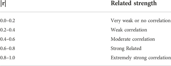
TABLE 1. Table of feature correlated intensity.

Feature correlation has a big impact on machine learning performance. The central hypothesis is that good feature sets contain features that are highly correlated with the class, yet uncorrelated with each other (Hall, 1999).

2.2.2 Feature derivation

In order to create additional features that are crucial to the model, derived features are created by leveraging the data’s original features. On the one hand from the business perspective, on the other hand from the machine learning model perspective.

With the use of statistical techniques and commercial expertise, new features are created from the original data in order to extract key information. For instance, if you are knowledgeable about the business logic, you may glean a lot of useful information from it. You can also glean incremental features from features with rather significant changes in feature values.

Feature derivation, which is also known as feature discretization, expands the value of a single feature to produce numerous features. The category characteristics must be encoded using one-hot encoding to produce multiple features before being fed into the linear model if one is utilized; The feature values for numerical features could be binned into a number of fixed interval segments, followed by the use of one-hot encoding to create the interval segments. Such a method can make it easier for features to be combined later.

The technique of combining two or more features in a certain way to create new features from a dataset is known as feature combination. Features are combined by feature intersection, which combines their intersection, concatenation, complementary, and Cartesian set intersection. Numerical operations include adding, removing, multiplying, and dividing features.

2.3 Machine learning methods

Machine learning is divided into two main parts: supervised learning (Breiman, 2001) and unsupervised learning (Friedman, 2001). To train a classification model that can discriminate between cats and dogs, for example, existing photos must be labeled to indicate whether each image is of a cat or a dog. Supervised learning requires labeled datasets for model training. The datasets are directly grouped via unsupervised learning, which eliminates the need to label the datasets; data inside the same group shares characteristics. The common models used in machine learning algorithms are classified as decision trees into regression decision trees (Hoerl and Kennard, 1970) and classification decision trees (Fletcher and Islam, 2019).

2.3.1 XGBoost

The premise behind the boost approach (Schapire, 1999), which was evolved from classification decision tree models, is that it is significantly simpler to train many models with low prediction accuracy than it is to train just one model accurately. The Boost algorithm uses its loss function to adjust the next weak learner after each training weak learner. The final model is obtained once the loss function has decreased to a predetermined small value.

By lowering the gradient of the prior weak learner in Boost (gradient = actual value - predicted value), GBDT (Ke et al., 2017) creates a new weak learner in the direction of gradient reduction (Schapire, 1999; Friedman, 2001; Ke et al., 2017). Following this GBDT sequentially constructs the weak classifier with reduced gradient.

The XGBoost (Chen and Guestrin, 2016) regression algorithm is derived from the GBDT algorithm, which is derived from the Boost regression algorithm. The benefit of XGBoost is that the loss function’s form may be customized, enhancing the model’s generalizability.

XGBoost has made a lot of advancements in order to raise the model’s efficacy. Among them include the employment of a regularization term to prevent model overfitting and the provision of column sampling to increase the model’s generalizability. The loss function of the model is also expanded from squared loss to second-order derivable function loss. The method of XGBoost uses the Taylor expansion quadratic term as the loss function, and the first two orders as the improved gradient; the regularization limits the complexity of the model, and a model with higher complexity is prone to lead to overfitting. This type of training produces a model with low error and strong outcomes on the training set, but it performs terribly on the test set and has poor generalization ability. The column sampling method can be employed in XGBoost to increase the model’s generalization capacity because it is comparable to the random forest feature sampling method.

The loss function and the regularization term make up the two components of the XGBoost objective function. The XGBoost objective function’s derivation is carried out below.

It is known that the training set $\mathrm{T}=\left\{\left({\mathrm{x}}_1,y_1\right),\left({\mathrm{x}}_2,y_2\right),\dots ,\left({\mathrm{x}}_n,y_n\right)\right\}$, the loss function $\iota \left(y_i,{\widehat{y}}_i\right)$, and the regularization term $\Omega \left(f_k\right)$ the overall objective function can be written as Eq. 6:

$\mathrm{O}\mathrm{b}\mathrm{j}={\displaystyle \sum }_i\text{ι}\left(y_i,{\widehat{y}}_i\right)+{\displaystyle \sum }_k\text{Ω}\left(f_k\right)(6)$

Where $\mathrm{O}\mathrm{b}\mathrm{j}$ is the expression on linear space; $i$ is the ith sample and $\mathrm{k}$ is the kth tree; and ${\widehat{y}}_i$ is the predicted value of the ith sample $x_i$. $\mathrm{O}\mathrm{b}\mathrm{j}$ can be translated into Eq. 7:

$\mathrm{O}\mathrm{b}\mathrm{j}={\displaystyle \sum }_i\text{ι}\left(y_i,{\widehat{y}}_i^{t-1}+f_t\left(x_i\right)\right)+{\displaystyle \sum }_k\text{Ω}\left(f_k\right)(7)$

Three steps to optimize the XGBoost objective function: first, the Taylor expansion of the objective function is carried out to the quadratic term and the constant term is removed, thus optimizing the loss function term to obtain Eq. 8:

$\mathit{O}\mathit{b}\mathit{j}={\displaystyle \sum }_{\mathit{i}=\mathbf{1}}^{\mathit{n}}\left[\mathit{\iota }\left({\mathit{y}}_{\mathit{i}},{\widehat{\mathit{y}}}_{\mathit{i}}^{\mathit{t}-\mathbf{1}}\right)+{\mathit{g}}_{\mathit{i}}{\mathit{f}}_{\mathit{t}}\left({\mathit{x}}_{\mathit{i}}\right)+\frac{\mathbf{1}}{\mathbf{2}}{\mathit{h}}_{\mathit{i}}{\mathit{f}}_{\mathit{t}}^{\mathbf{2}}\left({\mathit{x}}_{\mathit{i}}\right)\right]+{\displaystyle \sum }_{\mathit{k}}\mathit{\Omega }\left({\mathit{f}}_{\mathit{k}}\right)(8)$

Then, expanding the regularization term and removing the constant term yields Eq. 9:

$\mathit{O}\mathit{b}\mathit{j}={\displaystyle \sum }_{\mathit{i}=\mathbf{1}}^{\mathit{n}}\left[{\mathit{g}}_{\mathit{i}}{\mathit{f}}_{\mathit{t}}\left({\mathit{x}}_{\mathit{i}}\right)+\frac{\mathbf{1}}{\mathbf{2}}{\mathit{h}}_{\mathit{i}}{\mathit{f}}_{\mathit{t}}^{\mathbf{2}}\left({\mathit{x}}_{\mathit{i}}\right)\right]+\mathit{\Omega }\left({\mathit{f}}_{\mathit{k}}\right)(9)$

Next, combining the primary and quadratic coefficients yields Eq. 10:

$\mathit{\Omega }\left({\mathit{f}}_{\mathit{k}}\right)=\mathit{\gamma }\mathit{{\rm T}}+\frac{\mathbf{1}}{\mathbf{2}}\mathit{\lambda }{\displaystyle \sum }_{\mathit{j}=\mathbf{1}}^{\mathit{T}}{\mathit{w}}_{\mathit{j}}^{\mathbf{2}}(10)$

Bringing $f_t\left(x_i\right)=w_{q\left(x_i\right)}$ into the objective function yields Eq. 11:

$\mathit{O}\mathit{b}\mathit{j}={\displaystyle \sum }_{\mathit{i}=\mathbf{1}}^{\mathit{n}}\left[{\mathit{g}}_{\mathit{i}}{\mathit{w}}_{\mathit{q}\left({\mathit{x}}_{\mathit{i}}\right)}+\frac{\mathbf{1}}{\mathbf{2}}{\mathit{h}}_{\mathit{i}}{\mathit{w}}_{\mathit{q}\left({\mathit{x}}_{\mathit{i}}\right)}^{\mathbf{2}}\right]+\mathit{\gamma }\mathit{{\rm T}}+\frac{\mathbf{1}}{\mathbf{2}}\mathit{\lambda }{\displaystyle \sum }_{\mathit{j}=\mathbf{1}}^{\mathit{T}}{\mathit{w}}_{\mathit{j}}^{\mathbf{2}}(11)$

Taking all training samples and grouping them by leaf nodes yields Eq. 12:

$\mathit{O}\mathit{b}\mathit{j}={\displaystyle \sum }_{\mathit{i}=\mathbf{1}}^{\mathit{T}}\left[\left({\displaystyle \sum }_{\mathit{i}\in {\mathit{I}}_{\mathit{j}}}{\mathit{g}}_{\mathit{i}}\right){\mathit{w}}_{\mathit{j}}+\frac{\mathbf{1}}{\mathbf{2}}\left({\displaystyle \sum }_{\mathit{i}\in {\mathit{I}}_{\mathit{j}}}{\mathit{h}}_{\mathit{i}}+\mathit{\lambda }\right){\mathit{w}}_{\mathit{j}}^{\mathbf{2}}\right]+\mathit{\gamma }\mathit{{\rm T}}(12)$

Define Eqs. 13 and 14:

$G_j={\displaystyle \sum }_{i\in I_j}{g}_i(13)$

$H_j={\displaystyle \sum }_{i\in I_j}{h}_i(14)$

Bringing $G_j$ and $H_j$ into the objective function yields Eq. 15:

$\mathit{O}\mathit{b}\mathit{j}={\displaystyle \sum }_{\mathit{i}=\mathbf{1}}^{\mathit{T}}\left[{{\mathit{G}}_{\mathit{j}}\mathit{w}}_{\mathit{j}}+\frac{\mathbf{1}}{\mathbf{2}}\left({\mathit{H}}_{\mathit{j}}+\mathit{\lambda }\right){\mathit{w}}_{\mathit{j}}^{\mathbf{2}}\right]+\mathit{\gamma }\mathit{{\rm T}}(15)$

2.3.2 Stacking

One of the integrated learning approaches, along with bagging and boosting, is stacking. Where the k-fold cross-validation method is used to address the data leaking issue and output the samples for each component. Here, we implement the following design using 5-fold cross-validation as an example. In the beginning, the data is split into five segments, of which four are used as the training set and one as the validation set. A total of five models are then trained. Second, the models trained on the training set predict the validation set, and the prediction results are used as the input of the second layer model. Finally, there are five output values that are averaged and utilized as the input of the second layer after each trained model predicts the test set in step three. In order for the weak learners to complement one another’s strengths and be able to develop the ideal strong learner, the weak learners with less resemblance are chosen.

Input: Training set$\mathrm{D}=\left\{\left(x_1,y_1\right),\left(x_2,y_2\right),\dots ,\left(x_m,y_m\right)\right\}$

Elementary learning algorithms ${\mathfrak{L}}_1,{\mathfrak{L}}_1,\dots ,{\mathfrak{L}}_T$

Secondary learning algorithm $\mathfrak{L}$

Process:

1. for $\mathbf{t}=\mathbf{1,2},\dots ,\mathbf{T}$ do

2. $h_t={\mathfrak{L}}_t\left(D\right)$

3. End for

4. $D^{\prime }=\varnothing$

5. for $i=\mathrm{1,2},\dots ,m$ do

6. for $t=\mathrm{1,2},\dots ,T$ do

7. $z_{it}=h_t\left(x_i\right)$

8. End for

9. $D^{\prime }=D^{\prime }\cup \left(\left({\mathit{z}}_{\mathit{i}\mathbf{1}},{\mathit{z}}_{\mathit{i}\mathbf{2}},\dots ,{\mathit{z}}_{\mathit{i}\mathit{T}}\right),{\mathit{y}}_{\mathit{i}}\right);$

10. End for

11. $h^{\prime }=$ $\mathfrak{L}\left(D^{\prime }\right)$

12. Output: $H\left(x\right)=h^{\prime }\left(h_1\left(x\right),h_2\left(x\right),\dots ,h_T\left(x\right)\right)$

3 Proposed approach

3.1 Data pre-processing

The dataset underwent data pre-processing, such as data cleaning, data integration, data statute, and data transformation. We first sought advice from specialists in the field of materials before doing data preprocessing for machine learning.

First, the data with feature value of PAW_PBE in feature dft_type was selected. Then, the features identified after consultation with material domain experts that are not relevant to the bandgap valuesspecies_pp, species_pp_version, valence_cell_iupac, valence_cell_std, Egap_fit, energy_cutoff, delta_electronic_energy_convergence, kpoints, delta_electronic_energy_threshold, positions_fractional, bravais_lattice_orig, lattice_variation_orig, lattice_system_orig, Pearson_symbol_orig, Bravais_lattice_relax, lattice_variation_relax, lattice_system_relax, Pearson_ symbol_relax, others_json_type, all_json_type, attachment_file, created_at, updated_at, and deleted_at, etc.

3.1.1 Data cleaning

First, the attributes must be chosen and processed. Then, have to get rid of features that were made by combining other features (natoms, compound, dft_type), features whose element values are separated by commas and are messy and irregular, and features that are missing more than 80% of their values. Finally, you have to fill the empty values with the mean value of SpinF features.

Get rid of the columns of features that are missing more than 20% of their values. Using the logic behind the remaining feature values, we can figure out that the number of oxygen atoms needs to be filled. Using the periodic table of elements, we can find that the number of oxygen atoms needs to be set to 6. All of the missing vacancies in the feature species pp ZVAL are made of oxygen.

The compound can be made up of the composition and species to make future feature engineering easier and to make the input model more convenient. The feature compound can be removed.

The volume cell is equal to the product of the volume atom times the number of atoms. The energy cell is equal to the product of the energy atom times the number of atoms. The enthalpy cell is equal to the product of the enthalpy atom times the number of atoms. The PV cell is equal to the product of the PV atom times the number of atoms. Spin cell is the same as spin atom times the number of atoms. Stoich is the same as the ratio of the number of atoms of different elements in the compound. Spacegroup relax and spacegroup_orig are the same as spacegroup relax and spacegroup_orig.

The cost of training a model can be cut by getting rid of one of the features for characteristics that can be combined with other features or have the same feature value more than once.

3.2 Feature engineering

3.2.1 Characteristic analysis of variance

When the variance of the internal feature vector is 0, the feature does not give the model any more information. Following data preprocessing, the calculated variance of the attributes is displayed in Table 2.

TABLE 2

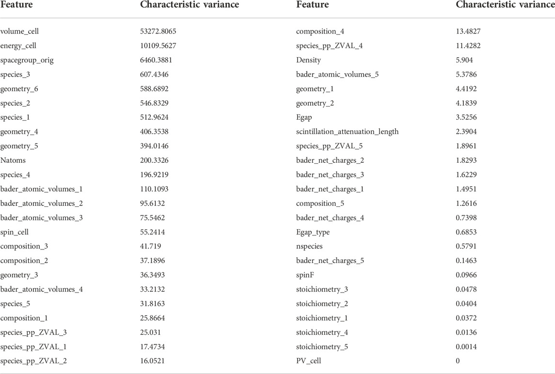
TABLE 2. Variance of feature.

In addition to evaluating the variance of the internal vector of the feature, the correlation of each feature must be calculated, which will speed up the construction of the machine learning model. So, the next will calculate the Pearson correlation of each feature.

3.2.2 Feature multicollinearity analysis

Multicollinearity between features during model training has a detrimental impact on the trained model scores, and this effect is particularly pronounced in linear models. In this study, we filter away the features whose absolute value of correlation is equal to one and keep one of them using Pearson’s coefficient of correlation approach. When multiple features are positively or negatively correlated with the same feature, it is sufficient to keep one feature.

The multicollinearity is computed using the Pearson correlation coefficient method, and the heat map of the derived Pearson correlation coefficient component is displayed in Figure 1.

FIGURE 1

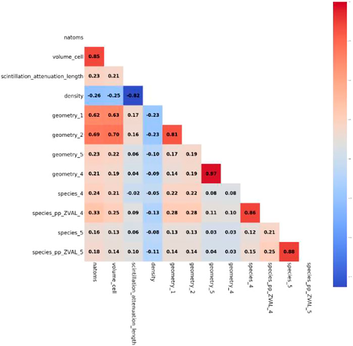
FIGURE 1. Heat map of features’ pearson correlation coefficient.

The correlation between natoms and volume cell is 0.85, according to the calculation of the Pearson correlation coefficient, the correlation coefficient between scintillation_attenuation_length and density is -0.82, the correlation between geometry_1 and geometry_2 The correlation coefficient between geometry_1 and geometry_2 is 0.81, the correlation coefficient between geometry_5 and geometry_4 is 0.97, the correlation coefficient between species_4 and species_pp_ZVAL_4 is 0.86, and the correlation coefficient between species_5 and species_pp_ZVAL_5 is 0.88. This work attempts to eliminate one of the extremely strongly associated aspects for these and their significantly correlated features. Table 3 displays the model assessment values of these features both before and after elimination.

TABLE 3

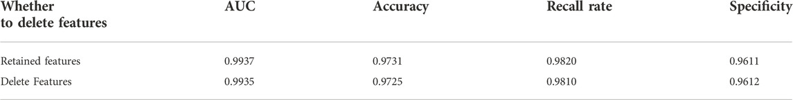
TABLE 3. The compare of whether to retain Strongly relevant features’ classification model.

The retention of these extremely strongly associated feature models is more productive, as shown by the assessment metrics of the aforementioned tests.

4 Machine learning experiments

In order to be more effective when using the model, the experimental protocol design should adhere to the original logic of the data business. In the area of material bandgap, there are also some physical laws. The law that states that bandgap values are 0 for metals and greater than 0 for nonmetals is revealed by a review of references and data exploration (Zhuo et al., 2018), and the data for material compounds with bandgap values of 0 and those with bandgap values greater than 0 are comparable. Additionally, the physical qualities of materials that share the same composition or structure are more similar.

Based on the above material characteristics two major types of scenarios are designed in this section. The process is shown in the Figure 2. The construction of methods for forecasting the bandgap values of metallic and non-metallic materials is the first major category, and it is further broken down into direct regression models, categorical regression models, and stacking procedures. The second major category of solutions is to design solutions for predicting non-metallic bandgap values, which comprise training the regression model, dividing the dataset into groups based on the different element kinds, and direct regression model prediction.

FIGURE 2

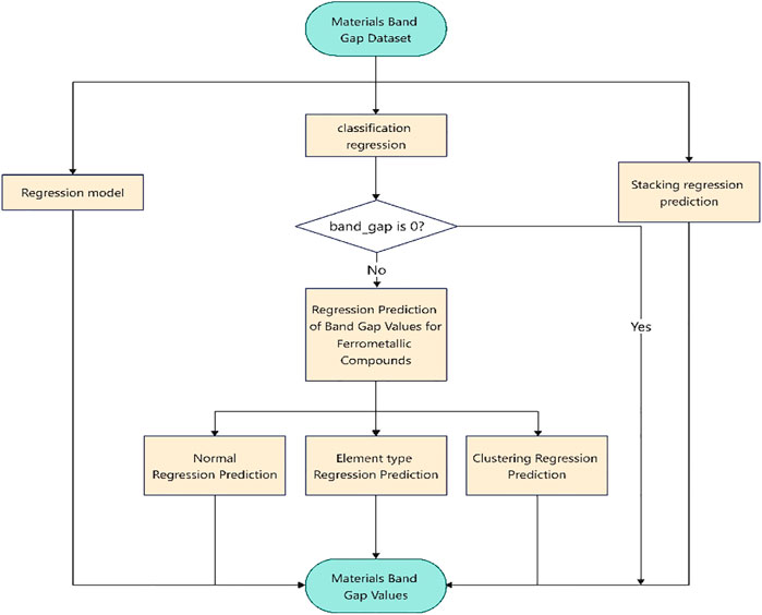
FIGURE 2. Experiment scheme flow chart.

4.1 Classification model

The partial confusion matrix obtained from the training model in 10-fold cross validation using the XGBoost classification algorithm is displayed in Figure 3. The distinction between metal and non-metal materials is almost perfectly made by the average AUC value of 0.9937. There is a 97.3% accuracy rate. The specificity is 0.9611 and the recall is 0.9820.

FIGURE 3

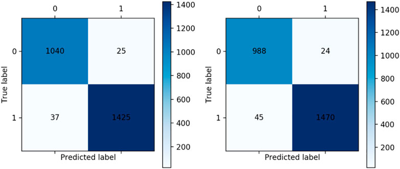
FIGURE 3. XGBoost 10-fold confusion Matrix.

Figure 4 displays the ROC curves that were generated using the ten-fold cross-validation procedure. The model’s area under the ROC curve is clearly visible in the figure, demonstrating that the model has a strong classification effect.

FIGURE 4

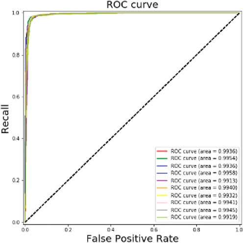
FIGURE 4. XGBoost 10-fold ROC.

4.2 Regression model

The experimental procedure and results of splitting the dataset according to the number of compound elemental species are described in detail. The scheme of dividing the dataset according to the compound elemental species performed best on the test set in predicting the regression model for non-metallic compounds. The non-metallic dataset contained in this dataset has 2, 3, 4, and five elemental compounds, so the regression model for predicting the four bandgap values was trained.

There are 14,457 non-metallic compound data available. The best model among the three models, XGBoost, random forest, and lightGBM, is now chosen for training prediction using a ten-fold cross-validation approach.

The evaluation metrics of the three regression models on the five datasets are shown in Figure 5.

FIGURE 5

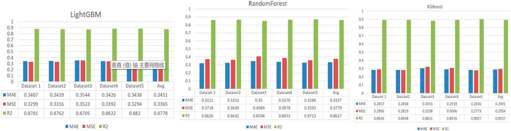
FIGURE 5. Three models evaluation metrics.

As shown in the Figure 6. By observing the average values of the evaluation metrics of the three models on the five test sets, it can be concluded that the XGBoost model has the best phenotype, so the XGBoost algorithm is better overall when training the regression model after splitting the dataset according to the number of element types.

FIGURE 6

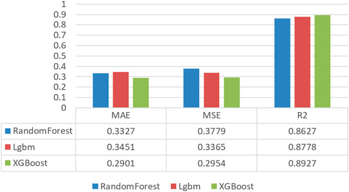
FIGURE 6. Evaluate metric of three regression models.

One dataset was chosen from five datasets to more clearly and visually demonstrate how the XGBoost model prediction affected the validation set, and the scatter plot of the bandgap values and the fitted curves were drawn for the true bandgap values of the training model on the validation set and the predicted bandgap values of the model on the validation set, so that the discrepancy between the model’s true bandgap values on the validation set and predicted bandgap values could be more easily compared with the true values. As a result, the model’s impact may be seen.

The model predicts the bandgap values, which are shown in the vertical coordinates. The real bandgap values, which were computed using the DFT method, are shown in the horizontal coordinates. As shown in the Figure 7, the gray straight line shows the best model, in which the predicted and real values are exactly the same when fitting the curve, and the orange straight line shows the line that shows how well the predicted and real values fit the scatter plot. When the gray line and orange line overlap more, the trained model works better. When they do not overlap as much, it does not work as well.

FIGURE 7

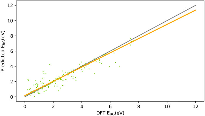
FIGURE 7. Fitted plot of two elemental compound predict Egap and DFT Egap.

5 Summary and conclusion

In this paper, the classifier that tells the difference between metal and non-metal is restarted using the training XGBoost model with machine learning method. This is done by starting with the physical properties of electronic slurries, which are the main material used to make devices for the intelligent power grid, and analyzing the data using bandgap theory. And the grid search algorithm is used to find the best value for the XGBoost model’s hyper parameters. The AUC value, accuracy, recall, and specificity are the four evaluation indexes that are used to decide what the best value is. After XGBoost tuning, the AUC of the model is 0.9943, which is better by 0.0006. The recall is 0.9815, which is worse by 0.0005, and the specificity is 0.9623, which is better by 0.0003. The accuracy is 0.9733, which is better by 0.0.

Data availability statement

Publicly available datasets were analyzed in this study. This data can be found here: http://aflowlib.org/search/?search=Au.

Author contributions

Conception and design of study: XL, YB Acquisition of data: ZY, XL Analysis and interpretation of data: XL, YB, FL Drafting the manuscript: ZY, XL, YB Revising the manuscript critically for important intellectual content: XL, YH.

Funding

The Major R & D Project of Yunnan Province, China (Grant No. 2018ZE001 and 202002AB080001-1).

Conflict of interest

The authors declare that the research was conducted in the absence of any commercial or financial relationships that could be construed as a potential conflict of interest.

Publisher’s note

All claims expressed in this article are solely those of the authors and do not necessarily represent those of their affiliated organizations, or those of the publisher, the editors and the reviewers. Any product that may be evaluated in this article, or claim that may be made by its manufacturer, is not guaranteed or endorsed by the publisher.

References

Ahn, S., Jung, S., Gwak, J., Cho, A., Shin, K., Yoon, K., et al. (2010). Determination of band gap energy (E g) of Cu 2 ZnSnSe 4 thin films: On the discrepancies of reported band gap values. Appl. Phys. Lett. 97 (2), 021905. doi:10.1063/1.3457172

CrossRef Full Text | Google Scholar

Breiman, L. (2001). Random forests. Mach. Learn. 45 (1), 5–32. doi:10.1023/a:1010933404324

CrossRef Full Text | Google Scholar

Chen, T., and Guestrin, C. (2016). “XGBoost: A scalable tree boosting system,” in Proceedings of the 22nd ACM SIGKDD international conference on knowledge discovery and data mining (San Francisco, California, USA: Association for Computing Machinery).

Google Scholar

Cohen, A. J., Mori-Sánchez, P., and Yang, W. J. C. r. (2012). Challenges for density functional theory. Chem. Rev. 112 (1), 289–320. doi:10.1021/cr200107z

PubMed Abstract | CrossRef Full Text | Google Scholar

Cover, T., and Hart, P. (1967). Nearest neighbor pattern classification. IEEE Trans. Inf. Theory 13 (1), 21–27. doi:10.1109/tit.1967.1053964

CrossRef Full Text | Google Scholar

Dong, Y., Cui, X., Zhang, L., and Ai, H. (2018). An improved progressive TIN densification filtering method considering the density and standard variance of point clouds. ISPRS Int. J. Geoinf. 7 (10), 409. doi:10.3390/ijgi7100409

CrossRef Full Text | Google Scholar

Fletcher, S., and Islam, M. Z. (2019). Decision tree classification with differential privacy: A survey. ACM Comput. Surv. 52 (4), 1–33. doi:10.1145/3337064

CrossRef Full Text | Google Scholar

Friedman, J. H. (2001). Greedy function approximation: A gradient boosting machine. Ann. statistics 29, 1189–1232. doi:10.1214/aos/1013203451

CrossRef Full Text | Google Scholar

Grinsztajn, L., Oyallon, E., and Varoquaux, G. (2022). Why do tree-based models still outperform deep learning on tabular data? arXiv preprint arXiv:. doi:10.48550/ARXIV.2207.08815

CrossRef Full Text | Google Scholar

Hall, M. A. (1999). Correlation-based feature selection for machine learning. Hamilton, New Zealand: The University of Waikato.

Google Scholar

Hauke, J., and Kossowski, T. (2011). Comparison of values of Pearson's and Spearman's correlation coefficients on the same sets of data. Quaest. Geogr. 30 (2), 87–93. doi:10.2478/v10117-011-0021-1

CrossRef Full Text | Google Scholar

Himanen, L., Jäger, M. O. J., Morooka, E. V., Federici Canova, F., Ranawat, Y. S., Gao, D. Z., et al. (2020). DScribe: Library of descriptors for machine learning in materials science. Comput. Phys. Commun. 247, 106949. doi:10.1016/j.cpc.2019.106949

CrossRef Full Text | Google Scholar

Hoerl, A. E., and Kennard, R. W. (1970). Ridge regression: Biased estimation for nonorthogonal problems. Technometrics 12 (1), 55–67. doi:10.1080/00401706.1970.10488634

CrossRef Full Text | Google Scholar

Jain, A., Ong, S. P., Hautier, G., Chen, W., Richards, W. D., Dacek, S., et al. (2013). Commentary: The materials Project: A materials genome approach to accelerating materials innovation. Apl. Mater. 1 (1), 011002. doi:10.1063/1.4812323

CrossRef Full Text | Google Scholar

Ke, G., Meng, Q., Finley, T., Wang, T., Chen, W., Ma, W., et al. (2017). Lightgbm: A highly efficient gradient boosting decision tree. Adv. neural Inf. Process. Syst., 3149–3157. doi:10.5555/3294996.3295074

CrossRef Full Text | Google Scholar

Lee, J., Seko, A., Shitara, K., Nakayama, K., and Tanaka, I. (2016). Prediction model of band gap for inorganic compounds by combination of density functional theory calculations and machine learning techniques. Phys. Rev. B 93 (11), 115104. doi:10.1103/physrevb.93.115104

CrossRef Full Text | Google Scholar

Ma, L., Li, N., Guo, Y., Wang, X., Yang, S., Huang, M., et al. (2021a). Learning to optimize: Reference vector reinforcement learning adaption to constrained many-objective optimization of industrial copper burdening system. IEEE Trans. Cybern. 1, 14. doi:10.1109/TCYB.2021.3086501

CrossRef Full Text | Google Scholar

Ma, L., Wang, X., Wang, X., Wang, L., Shi, Y., and Huang, M. (2021b). Tcda: Truthful combinatorial double auctions for mobile edge computing in industrial internet of things. IEEE Trans. Mob. Comput. 1, 1. doi:10.1109/TMC.2021.3064314

CrossRef Full Text | Google Scholar

Matsuoka, T., Okamoto, H., Nakao, M., Harima, H., and Kurimoto, E. (2002). Optical bandgap energy of wurtzite InN. Appl. Phys. Lett. 81 (7), 1246–1248. doi:10.1063/1.1499753

CrossRef Full Text | Google Scholar

Park, C., and Heo, W. (2020). Review of the changing electricity industry value chain in the ICT convergence era. J. Clean. Prod. 258, 120743. doi:10.1016/j.jclepro.2020.120743

CrossRef Full Text | Google Scholar

Pilania, G., Mannodi-Kanakkithodi, A., Uberuaga, B., Ramprasad, R., Gubernatis, J., and Lookman, T. (2016). Machine learning bandgaps of double perovskites. Sci. Rep. 6 (1), 19375–19410. doi:10.1038/srep19375

PubMed Abstract | CrossRef Full Text | Google Scholar

Plutowski, M., and White, H. (1993). Selecting concise training sets from clean data. IEEE Trans. Neural Netw. 4 (2), 305–318. doi:10.1109/72.207618

PubMed Abstract | CrossRef Full Text | Google Scholar

Rabek, J. F. (2012). Photodegradation of polymers: Physical characteristics and applications. Springer Science & Business Media.

Google Scholar

Radisavljevic, B., Radenovic, A., Brivio, J., Giacometti, V., and Kis, A. (2011). Single-layer MoS2 transistors. Nat. Nanotechnol. 6 (3), 147–150. doi:10.1038/nnano.2010.279

PubMed Abstract | CrossRef Full Text | Google Scholar

Schapire, R. E. (1999). “A brief introduction to boosting,” in Proceedings of the sixteenth international joint conference on artificial intelligence Stockholm, Sweden (Morgan Kaufmann Publishers Inc), 1401–1406.

Google Scholar

Schubert, E. F., and Kim, J. K. (2005). Solid-state light sources getting smart. Science 308 (5726), 1274–1278. doi:10.1126/science.1108712

PubMed Abstract | CrossRef Full Text | Google Scholar

Wei, J., Chu, X., Sun, X.-Y., Xu, K., Deng, H.-X., Chen, J., et al. (2019). Machine learning in materials science. InfoMat 1 (3), 338–358. doi:10.1002/inf2.12028

CrossRef Full Text | Google Scholar

Xie, T., and Grossman, J. C. (2018). Crystal graph convolutional neural networks for an accurate and interpretable prediction of material properties. Phys. Rev. Lett. 120 (14), 145301. doi:10.1103/physrevlett.120.145301

PubMed Abstract | CrossRef Full Text | Google Scholar

Yiwei, A., Yunxia, Y., Shuanglong, Y., Lihua, D., and Guorong, C. (2007). Preparation of spherical silver particles for solar cell electronic paste with gelatin protection. Mater. Chem. Phys. 104 (1), 158–161. doi:10.1016/j.matchemphys.2007.02.102

CrossRef Full Text | Google Scholar

Zeng, Y., Chua, S. J., and Wu, P. (2002). On the prediction of ternary semiconductor properties by artificial intelligence methods. Chem. Mat. 14 (7), 2989–2998. doi:10.1021/cm0103996

CrossRef Full Text | Google Scholar

Zhaochun, Z., Ruiwu, P., and Nianyi, C. (1998). Artificial neural network prediction of the band gap and melting point of binary and ternary compound semiconductors. Mater. Sci. Eng. B 54 (3), 149–152. doi:10.1016/s0921-5107(98)00157-3

CrossRef Full Text | Google Scholar

Zhuo, Y., Mansouri Tehrani, A., and Brgoch, J. (2018). Predicting the band gaps of inorganic solids by machine learning. J. Phys. Chem. Lett. 9 (7), 1668–1673. doi:10.1021/acs.jpclett.8b00124

PubMed Abstract | CrossRef Full Text | Google Scholar