Economic Impacts of the U.S. Renewable Fuel Standard: An Ex-Post Evaluation

Introduction

When a government imposes a regulation, it usually indicates that policy makers believe that the market would not produce the socially desired outcome. The U.S. Renewable Fuel Standard (RFS) is a good example of such a regulation. Congress believed that markets would not produce the “desired” amounts of renewable fuels, so it established requirements for minimum levels of use of different kinds of renewable fuels, providing biofuels access to the fuels market. However, it is not always the case that the mandate becomes binding if market conditions change. It is possible that with unforeseen changes in market conditions, a biofuel would be produced and/or used due to market forces, at least to some extent. This paper examines the extent to which biofuel production has been driven through time primarily by the RFS, and the extent to which it was driven by market changes unforeseen at the time of RFS passage.

The original RFS was enacted by Congress in 2005 (U.S. Congress, 2005). It was amended in 2007, and the revised and current RFS is sometimes referred to as RFS2 (U.S. Congress, 2007). However, in this paper, we will refer to it as RFS. The major objectives of the RFS were 1) to provide a source of increased incomes and employment in rural areas, 2) to increase US energy security, and 3) to reduce greenhouse gas (GHG) emissions (Tyner, 2012). However, prior to the enactment of the RFS, there was other legislation related to ethanol, which is summarized by Tyner (2008). The National Energy Conservation Policy Act (U.S. Congress, 1978) was essentially the first piece of renewable energy legislation and established an excise tax exemption for ethanol of $0.40/gal.¹ This tax incentive was converted to a Volumetric ethanol Excise Tax Credit (VEETC) in the American Jobs Creation Act of 2004 (U.S. Congress, 2004). The government support continued in some form through 2011 and varied between $0.40 and $0.60/gal. of ethanol. The use of government incentives and the RFS were the two main policy instruments aimed at helping to establish and grow the ethanol industry to accomplish the three aforementioned goals. However, as described in this paper, there were many other factors that helped drive biofuel industry to grow since 1980.

Determining the economic impacts of the RFS is a complicated task. Part of the complication is the questions of attribution. For example, some of the early literature tended to blame the RFS for all increases in commodity prices. However, over time it has become abundantly clear that many factors have been involved in the evolution of commodity and food prices, with the RFS and biofuel production in general being only one.

The Supplementary Material (SM) of this paper provides a comprehensive literature review and data analysis to highlight the major debates in this area and review the historical trends in the key variables that sketch the interactions between the RFS and markets for energy and agriculture products. The SM divides the historical analyses into five periods that are characterized by different drivers, as shown in Supplementary Table S1.

The first period is 1980–2004. The only ethanol incentive during this period was the ethanol tax exemption, varied from 40 to 60 cents (Tyner, 2008). However, the Clean Air Act Amendments of 1990 also provided some demand for ethanol as a source of oxygen in gasoline (U.S. Congress, 1990). Prior to 2004, the price of crude oil was relatively low ranging from $10 to $33 per barrel (Supplementary Figure S2) and the price of corn was also usually low ranging from $1.4 to $4.4 per bushel (Supplementary Figure S3). Between 1983 and 2005, prior to enactment of RFS, the annual growth rate of demand for ethanol was about 9.5% (Tyner, 2008; Hertel et al., 2010) due to favorable market conditions such as low corn price, ethanol tax exemption, and demand for ethanol as an oxygen additive.

The second period is 2004–2008. Lots of things were changing during this period. The first RFS was passed in 2005, but it was not really binding in this period, except for 2008. A mandate is considered to be binding if it results in changes in production from what the market would have produced absent the mandate. In the case of the RFS, an indication of the extent to which the RFS is binding can be the price of Renewable Identification Numbers (RINs). If RINs prices are very low, it means the RFS is not playing a major role in determining production levels (Abbott, 2014). The ethanol RIN price was usually lower than five cents per gallon in this period, confirming a non-binding mandate. In this period the wholesale gasoline price sharply increased from $1.05 per gallon in January 2004 to $3.35 per gallon in July 2008 (Supplementary Figure S7). The ban on the use of Methyl Tertiary-Butyl Ether (MTBE), a toxic gasoline additive, has been passed in June 2006. This significantly increased demand for ethanol as a cheap and non-toxic substitute for MTBE, which helped ethanol industry to grow faster. In this period, ethanol production grew at a substantial 24% annual rate.

In this period commodity, and food prices generally increased. Various papers have studied the key drivers of commodity and food price increases that occurred in this time period (a few examples are: Delgado, 2008; Henderson, 2008; Trostle, 2008; and many more). Abbott et al. (2008) have reviewed many of these papers and concluded that the commodity and food price increases had three main sets of drivers for this time period: global changes in production and consumption of key commodities; the depreciation of the US dollar (exchange rate); and growth in production of biofuels.

The third period is 2008–2009. The great global recession began in this period. Many of the key drivers that had operated in the period leading up to 2008 went into reverse. Crude oil and gasoline prices plummeted (see Supplementary Figures S6, S7). With reduced global incomes, demand for most commodities and their prices fell. With declining gasoline prices, the price of ethanol followed. However, ethanol production remained strong because corn price fell along with or even further than ethanol prices. Though the recession was quite deep, commodity prices generally began a rebound in 2009. Throughout this period, ethanol RIN prices remained low suggesting again that the RFS was not binding in this period.

The fourth period is 2010–2011. Commodity prices again rose in this period, with crude oil topping $100 per barrel. During this period, some of the key drivers from earlier periods remained, but there were also new drivers (Abbott et al., 2011). Poor harvests in several parts of the world were more important in 2011 than in 2008 leading to higher agricultural commodity prices. Leading up to 2011 there was also a significant change in Chinese policy with respect to soybean imports. With persistent demands for corn for biofuels and China for soybeans, overall price elasticity became more inelastic, which led to higher prices and more price volatility. Ethanol and corn prices rose together in 2010–11. Blend wall concerns began to appear in 2011 (Tyner and Viteri, 2010; Abbott, 2014), but ethanol exports increased substantially over that period (see Supplementary Figure S9). As shown in Supplementary Figure S11, RIN prices for ethanol continued at low levels, indicating that the RFS still was not binding for ethanol. However, RIN priced for biodiesel surged, indicating a binding RFS for this biofuel (see Supplementary Figure S11).

Another development that began around 2009 was that ethanol prices moved below gasoline prices (Supplementary Figure S7) and appeared poised to remain low for some time. Many refiners saw this as an opportunity to reduce refining costs by producing lower-cost 84 octane gasoline out of the refinery and blending with 10 percent ethanol to yield an 87-octane blend at the pump. In fact, ethanol prices did remain below gasoline for years to come, and that change increased the market demand for ethanol as an octane additive. In other words, ethanol became more a standard part of the gasoline refining system. Ethanol has higher value as a fuel additive (oxygen and octane) than as a fuel extender, but this value is difficult to capture in economic models. However, in a recent FarmDoc Daily post, Scott Irwin quantified the added value ethanol provides as an octane enhancer (Irwin, 2019).

The fifth period is 2011–2016. In this period production of ethanol did not grow as before due to changes in market force. In 2012, the US experienced a major drought which led to a high corn price and negative ethanol margins according to the iowa State ethanol Profitability model and as illustrated in Supplementary Figure S10 (Agricultural Marketing Resource Center, 2019). As a consequence, ethanol production and exports declined (Supplementary Figures S1, S9).

During this period the gasoline consumption did not grow as it was expected due to two main factors. First, the great recession of 2008–09 led to a large drop in gasoline consumption, and consumption growth did not pick up for a considerable amount of time. Second, the US enacted more stringent fuel economy standards, which meant consumers could drive more miles with less fuel. High oil and gasoline prices also encouraged consumers to purchase more fuel-efficient vehicles and perhaps to drive slightly less. Due to these changes, the gasoline market moved towards the historical definition of the blend wall, the 10% maximum ethanol content (Tyner W. et al., 2010; Tyner W. E. et al., 2010; Tyner, and Viteri, 2010). Because of the decline in gasoline consumption, not enough ethanol could be blended at the historical 10% maximum ethanol content to achieve the implied RFS targets starting in 2013 (see Section 1.5 of the MS for details).

As mentioned before, prior to 2011, ethanol was basically in demand as a fuel extender and an octane additive. This changed after 2011 and a portion of ethanol was consumed as a substitute for gasoline to meet the RFS requirements, along with providing a source of octane. Since 2011, as the total consumption of ethanol moved towards the historical 10% maximum ethanol content (that was allowed in non-flex-fuel vehicles), demand for ethanol did not grow due to market forces enough to meet the minimum RFS requirement, and that led to higher RINs prices. Starting in 2013, the market observed major increases in the corn ethanol RIN values, as shown in Supplementary Figure S11. Starting in 2013 ethanol RIN prices moved up to biodiesel RIN prices and essentially followed biodiesel until recently as shown in Supplementary Figure S11. The RFS and historical 10% blend rate became the limiting factor until 2016. Due to the nested structure of the RFS, biodiesel and other advanced RINs could be used to satisfy the part of the conventional fuel (ethanol) requirement (adjusted and implied by the EPA) that could not be done with ethanol. Korting et al. argue that in addition to the RFS nested structure, the joint gasoline and diesel compliance base is also important (Korting et al., 2019).

Another important change in energy markets that occurred during this time period and negatively affected profitability of ethanol is the shale oil boom (Taheripour et al., 2014), which led to a 57% increase in US crude oil production between 2011 and 2016 (Supplementary Figure S12). This remarkable increase in US production helped push world crude oil prices lower as shown in Supplementary Figure S2, (for details see Section 1.5 of the SM).

In addition to dividing the literature and data analysis into the periods mentioned above, the SM also discusses other papers that provide a somewhat different take on the RFS such as one by Abbott (2014). It also covers other important papers that examine the time varying relationship between biofuels and commodity and food prices.

USDA has published some important papers on the food-fuel issue (Trostle, 2008; Trostle et al., 2011). There have been many econometric studies of the relationships among prices of crude oil, gasoline, ethanol, corn, and other commodities (Zhang et al., 2010; Wright, 2011; Chiou-Wei et al., 2019; Filip et al., 2019). Filip et al. (2019) have provided a review of much of the econometric literature. In addition, these authors used a comprehensive data set covering many commodities and other variables and concluded that: 1) ethanol did not affect agricultural commodity prices prior to the 2008 food crisis; 2) during the food crisis periods about 15 percent of the variance in corn prices was due to ethanol and 5 percent of other commodities; 3) after the food crisis, ethanol contributed about 10 percent of the variability in agricultural commodity prices; 4) biofuels did not serve as a leading source of high commodity prices. Finally, Filip et al. (2019) have asserted that their results serve as an “ex-post correction” of the previous results suggesting dramatic effects of biofuels on commodity and food prices. It is important to note that these authors have not separated impacts of the RFS from other market factors driving biofuels. It is just an analysis of the impacts and commodity price linkages due to biofuels regardless of whether the biofuels were driven by market forces or the RFS or some combination. For further discussion on the price impact of RFS see Sections 1.6 and 1.7 of the SM.

The main take-away from the literature review and analyses provided in the SM is that most of the analyses that have been done to date do not distinguish between market drivers of ethanol production growth and the RFS as a driver. In the 1980s and 1990s, ethanol tax incentives and the Clean Air Act Amendments of 1990, which established reformulated gasoline, were the key policies enabling establishment and relatively slow growth of the industry during a period of low crude oil prices. In the years 2004–08, there was a substantial run-up in crude oil prices that pulled ethanol into the market. The crude oil price increase and the 2006 MTBE ban were the key drivers in capacity additions. Ethanol margins were strong in 2005–07, which provided strong incentives to add capacity. Of course, the added ethanol production increased demand for corn and was part of the reason for the corn and other commodity price increases. Filip et al. (2019) have estimated that biofuels may have been responsible for about 15 percent of the rise in corn prices. But that was biofuels production induced primarily by market forces, and the ethanol tax incentive. Price correlations continued strong through the recession and the second commodity price surge in 2011. The 2012 drought reduced US corn production, and higher prices sent ethanol margins negative and led to a temporary drop in ethanol production. The short-run impact of biofuels on commodity prices may have been more important in late 2008 and early 2009. Since 2013 RIN prices increased rapidly due to constraints on the growth of ethanol consumption, as the market moved towards the 10% historical blend rate. Ethanol exports started a growing trend in 2013 that continued until 2019, when this research has been developed.

The literature review and analyses provided in the MS confirm that biofuels production being driven mainly by market forces and government support for ethanol, which ended in 2011. Prior to this year, the RFS provided an incentive to get capacity built and also generated a safety net for biofuels to grow, but it was not binding in the markets except for a few months in 2008–09. Since 2011, the RFS in combination with constraints on the growth of ethanol consumption drove the markets for biofuels. Finally, the recent econometric evidence suggests that biofuels were not the main driver of commodity price increases, (for detail see the SM).

A crucial question to ask given our conclusions on the role of markets in driving biofuels growth is How it would have been different if all these market changes had not occurred. In other words, what if crude oil price had not surged, MTBE had not been banned, ethanol did not get integrated into the fuel system becoming a fuel additive instead of a fuel extender, etc.? The answer is clearly that the RFS would have played a much greater role. So, in a sense, the RFS has been the backstop, but by circumstance, it was overpowered by tax incentives and market forces through 2011. Another important comparison is between what happened over this period for ethanol compared with biodiesel and cellulosic biofuels. For both biodiesel and cellulosic biofuels, the original mandated levels have not been implemented in practice and frequently revised over time. Hence, the RFS has not reached its original goals for these biofuels. However, after the waivers, the RFS was still clearly an important driver of production and consumption. RIN prices were always relatively high, and the RFS was always binding. Clearly, the market changes that benefitted ethanol did not work as much in favor of these other biofuels.

While the existing literature indicates that the RFS has played a critical role in providing a secure environment to produce and use more biofuels, to the best of our knowledge, no major effort has been made to isolate the economic impacts of this policy for other factors that helped the biofuel industry to grow. While, in general, the existing literature has successfully identified the key drivers of the growth in biofuels, it basically has failed to properly quantify the impacts and contributions of each of these drivers separately. This paper takes primary steps to fill this knowledge gap. Following an extensive literature review, it develops short- and long-run economic analyses, using Partial Equilibrium (PE) and Computable General Equilibrium (CGE) models, to differentiate the economic impacts of the RFS from other drivers that have helped biofuels to grow. Unlike the existing PE and CGE modeling efforts that typically provided ex ante economic analyses for biofuels, this paper follows Taheripour et al. (2019) and develops a new approach that uses actual observations for the time period 2004–16 to construct ex-post historical baselines and counterfactual simulations to achieve the goals of this research. The existing literature has addressed the economic impacts of biofuel production and policy from different perspectives including but not limited to: welfare gains and loses; demand for and supply of transportation fuels; fuel prices; food and commodity prices; and contributions to agricultural resource utilization. This paper concentrates on the last two topics of this list and provides new important and critical insights in these areas. It is important to note that the immediate price impacts of the RFS (e.g., monthly price impacts) could provide important insights on immediate price responses. However, our partial and general equilibrium modeling frameworks are not suitable for this type of analyses.

The literature review, data analysis, and modeling practices provided in this paper shows that: 1) while the RFS has played a critical role in providing a secure environment to produce and use more biofuels, at least in the 2000s, it was not the only factor that encouraged the biofuel industry to grow; 2) since 2011, the RFS in combination with constraints on the growth of ethanol consumption drove the markets for biofuels; 3) the medium-to long-run price impacts of biofuel production were noticeable, while the RFS had minor impacts on crops and food prices; 4) over time, biofuel production and policy made major contributions to the agricultural sector to utilize its resources more efficiently and that significantly improved farm incomes in the US; 5) biofuel production, regardless of the drivers, has increased the US annual farm incomes by $8.3 billion between 2004–11 with an extra additional annual income of $2.3 billion between 2011–2016; 6) the modeling practices provided in this paper assign 28% of the expansion in farm incomes of the period of 2004–2011 and 100% of the extra additional incomes of the period of 2011–16 to the RFS; and finally, the RFS as a backup policy has provided a secure environment for biofuel producers and that reduced policy uncertainties, which facilitated capacity generation and investment in biofuel industry in 2000s.

The rest of this paper is organized into three sections. First, we explain the approach we will use in this analysis. After that we will present the quantitative results of our model simulations and relate them to the literature and data discussions. The last section covers the conclusions.

Materials and Methods

To assess the annual, short-run, and long-run price impacts of the US RFS, in this research, we make use of both a Computable General Equilibrium (CGE) model and a Partial Equilibrium (PE) model. Each modeling approach has advantages and disadvantages, and we use each model relying on its unique strengths and fit for the question(s) being asked. In general, GTAP-BIO is used for the global and longer-term analysis, whereas the PE model is used for specific analysis of the US agricultural and liquid fuel sectors to capture finer and shorter-term impacts. The combination of the two modeling frameworks permits us to analyze and evaluate all the important issues related to biofuels, RFS, and commodity and food prices. We use the models iteratively in the analysis to gain the advantages of both approaches.

Computable General Equilibrium Model

To accomplish the goals of this paper, we will use a well-known global CGE model: GTAP-BIO. This model is an advanced version of the standard GTAP model. The standard model is fully described in Hertel (1997). GTAP-BIO extends the capabilities of the standard model to develop economic and land use analyses related to the environmental, agricultural, energy, trade, and biofuel policies and actions. This model has been improved over time and used in various applications (Taheripour and Tyner, 2011; Beckman et al., 2012; Taheripour and Tyner, 2013; Taheripour and Tyner, 2014; Taheripour et al., 2016b; Brookes et al., 2017; Taheripour and Tyner, 2018; Yao et al., 2018). Taheripour et al. (2017b) described the background of this model and Taheripour et al. (2017a) developed the latest version of this model.

This model traces production, consumption, and trade of all goods and services (aggregated into various categories) at the global scale. Unlike the standard model, GTAP-BIO disaggregates oil crops, vegetable oils, and meals into several categories including: soybeans, rapeseed, palm oil fruit, other oil seeds, soy oil, rapeseed oil, palm oil, other oils and fats, soy meal, rapeseed meal, palm kernel meal, and other meals. In addition to the standard commodities and services, this model integrates the production and consumption of biofuels (e.g., corn ethanol, sugarcane ethanol, and biodiesel) and their by-products (DDGS and meals). Therefore, unlike the standard GTAP model, the enhanced model takes into account the use of commodity feedstocks for food and fuel and the competition or trade-offs between those and other market uses. In addition, it traces land use (and changes in land prices) across the world at the level of Agro-Ecological Zone (AEZ). The latest version of this model handles intensification in crop production due to technological progress, multi-cropping, and conversion of unused cropland to crop production. Finally, the parameters of this model were calibrated to recent observations. This model traces the inter-relationships among crop, livestock, feed, and food sectors and links them with biofuels sectors and accounts for upstream and downstream linkages among these sectors and other economic activities. This model also considers resource constraints and technological progress. Hence, it provides a comprehensive framework to assess the price impacts of biofuel production and policies. While the GTAP-BIO model produces global outputs, for the purposes of this analysis, we focus on the US impacts.

Partial Equilibrium Model

The CGE analyses developed in this paper provide comprehensive and overall medium-to long-run analyses of the price impacts of the US RFS and do not include short-run and annual price changes induced by the RFS or other factors. The literature is rich with explanations of key drivers of price changes that may not be included in medium-to long-term models. A good example is the series of Farm Foundation papers that explain how the drivers of commodity and food price changes over the period 2008–2011 (Abbott et al., 2008; Abbott et al., 2009; Abbott et al., 2011). To provide short-run and annual analyses we will use an improved version of an Agricultural Energy Partial Equilibrium (AEPE) model which was developed by Taheripour and Tyner and used in several publications (Tyner and Taheripour, 2008; Tyner W. et al., 2010; Taheripour et al., 2016a) to examine interactions between agricultural and energy markets and evaluate the consequences of changes in biofuel policies. The improved version of the model covers crude oil, gasoline, corn ethanol, biodiesel, corn, soybeans, and feed (e.g., DDGS and meals) markets. The model is for the US economy. It distinguishes demand for corn and soybeans in their alternative uses (food, feed, biofuels, and exports) and traces changes in agricultural subsidies and biofuel policies.

The AEPE model uses a base year data set and short-run demand and supply elasticities for the (commodity) markets included in the model, and long-run and short-run shift factors in demand and supply of each market and determines their new equilibriums over time. The long-run and short-run shift factors are exogenous to this model. The long-run shift factors (e.g., population, income growth, and growth in demand for livestock products) help the model to adjust overtime. The short run shift factors represent annual exogenous changes (e.g., reductions in crop yields due to a drought). We have used this model for the time period 2004 to 2016 to better characterize short-run changes in the agricultural and fuel markets over this period. Some of the shift factors are directly observable, while others may not be directly observable. For example, historical data represent annual fluctuations in crop yields or changes in ethanol incentives are directly observable. The PE model takes into account these shift factors through its exogenous variables. For unobservable shift factors (e.g., shift factors in the demand of energy or shifts in foreign demand for corn), we will rely on the outputs of the GTAP-BIO model and other observations as discussed later in this paper.

Overall Modeling Approach

In essence, we use the AEPE model to provide more detailed results for the US than is possible from a global CGE model. The combination of the CGE and PE models and their results enables us to respond to most the goals of this project. Figure 1 represents our modeling approach and the links between the CGE and PE models. The CGE model results are used to assess the medium-to long-run price impacts of biofuels. The PE model assesses the annual and short-term price impacts of biofuels, including corn ethanol and soybean biodiesel. This figure shows interactive links between the CGE and PE models through the shift factors.

FIGURE 1

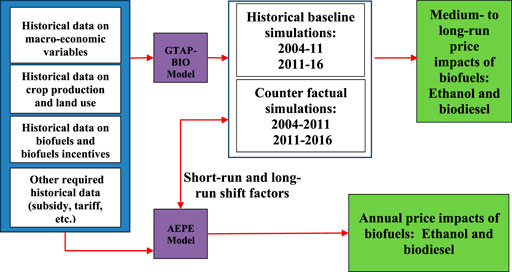
FIGURE 1. The overall modeling approach.

Examined Experiments

As described above, the main goal of this research is to answer the following important questions:

1) To what extent the RFS alone has affected commodity and food prices,

2) To what extent the expansion in US biofuel production has affected commodity and food prices, regardless of the causes,

3) To what extent the RFS alone has contributed to agricultural resource utilization,

4) To what extent the expansion in US biofuel production has contributed to agricultural resource utilization, regardless of the causes.

To answer these questions, we developed historical simulations and counterfactual experiments using the CGE and PE models. Essentially, we modeled what happened in the agricultural and energy sectors due to all causal factors. Then, we removed the RFS to determine what the impact of the RFS had been isolated from all the other market drivers of changes in these markets. Then, we removed biofuels production increases to determine what had been the impact of biofuels (whether driven by the RFS or other factors). In each case, the difference between the simulated historic baseline and the experiment gives us the impacts on prices, production, etc., due to the one factor that was being altered. The historical simulations capture and represent changes in economic variables as happened in the real world. The counterfactual experiments repeat the baseline simulations under alternative assumptions to capture the RFS/biofuel impacts from the impacts of other drivers. In what follows we describe the baselines and counterfactual experiments, first for the CGE approach and then for the PE method.

Computable General Equilibrium Baselines and Counterfactual Experiments

During the time period of 2004–2016, crop and food prices followed increasing trends until 2012 and then traced downward paths or remained relatively flat in the US. One can observe a similar pattern globally as well. Given this observation, since one goal of this research is to determine the impacts of the RFS on crop and food prices, we split the CGE analyses into two distinct time segments of 2004–2011 and 2011–2016 to better understand the differences between the price determining forces of these time periods. Therefore, for each of these time slices we developed several historical and counterfactual experiments.

Historical Baselines: A historical baseline in a typical static CGE analysis captures and represents changes in the global economy for a given observed time period, say 2004–11 or 2011–2016 in our analysis. To construct a historical baseline using a static CGE model, we exogenously shock the model for a given set of variables (including macroeconomic and policy variables) and allow the model to determine changes in the production, consumption, and trade for all goods and services (including crops and food items) and also prices by region². A baseline simulation usually takes into account technological progress in production of goods and services as well. Changes in Total Factor Productivity (TFP) and improvements in productivities of the primary and intermediate inputs usually represent technological progress.

To construct the historical baseline for each time period we closely followed the approach used by Yao et al. (2018). These authors developed a static historical baseline for the time period of 2004–2011 for a different application. Following these authors, in constructing the historical baseline for each time period, we exogenously shocked the model for the regional observed changes in population, gross domestic product (GDP), capital formation, labor force, managed land, biofuel production and policy, and agricultural and trade policies. We then allow the model to determine changes in the production, consumption, and trade for all goods and services (including crops and food items) and also prices by region. Given these exogenous shocks, the model determines TFP by country³. Given that technological progress in agriculture is a key driver of crop prices, we use observed changes in crop supplies to determine the rate of technological progress in crop sectors⁴. As mentioned in the literature review section, there were major shifts in crop demands between 2004 and 2016. Hence, in addition to the changes in crop yields, some demand shifters were introduced in the simulation processes for crop demands. Finally, the crude oil industry has changed significantly over the period 2004 to 2016. Since GTAP cannot capture these changes endogenously, we added proper shifters (shocks) to capture major changes in the oil market exogenously. Finally, as mentioned in the next section we obtained data from credible sources including but not limited to the World Bank, Food and Agricultural Organization of the United Nations (FAO), Organization for Economic Cooperation and Development (OECD), and USDA to calculate the implemented shocks for the baseline construction process of each time period.

To isolate the impacts (e.g., price impact) of the RFS from all other drivers that may affect production of biofuels we developed the following counterfactual experiments:

RFS Baseline: The historical baseline, among all drivers, captures the impacts of biofuel production on commodity and food prices. However, a portion of ethanol produced in the US was not used domestically. In 2011 and 2016 the US net export of ethanol was about one billion gallons and 1.1 billion gallons. Given that the RFS targets domestic consumption of ethanol, we eliminated the impacts of trade of ethanol from the historical baseline of each time period. In this experiment we freeze trade of ethanol to remain at its initial levels in the base year for each time slice. The difference between this experiment and the historical baseline captures the trade impacts of biofuels.

Counterfactual I- ethanol free of Mandate: This experiment repeats the RFS baseline while removing the restriction on ethanol consumption and allows market forces to determine ethanol consumption. For each time period, the difference between the RFS baseline and this counterfactual experiment represents the impacts of RFS for conventional ethanol.

Counterfactual II-No RFS: This experiment repeats the RFS baseline while removing the restriction on consumption of both ethanol and biodiesel and allows market forces to determine consumption of these biofuels. The difference between RFS baseline and this counterfactual experiment represents the impacts of RFS for both ethanol and biodiesel.

Figure 2 provides a schematic picture for these counterfactual experiments and their relationships with the historical baseline for each time period of 2004–11 (left panel) and 2011–16 (right panel). Consider the left panel of this figure, which represents the historical and counterfactual simulations with the solid black lines. The vertical axis shows the price of a representative product. For example, $P_{2011}^2$ and $P_{2011}^4$ indicate the projected price of this product in 2011 for the RFS baseline and No RFS cases, respectively. The difference between these two prices represents the impact of RFS on the price of the representative product for the time period of 2004–11.

FIGURE 2

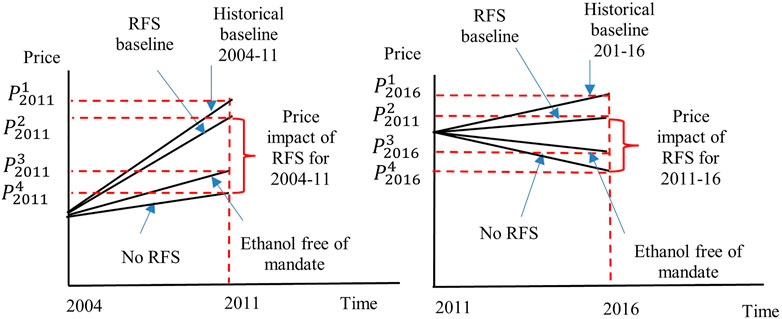
FIGURE 2. A schematic representation of historical baselines and counterfactual experiments including: FRS Baselines, ethanol free of mandate, and no RFS. The left panel represents 2004–11 and the right panel 2011–16. The vertical axis shows the price of a representative product. P¹, P², P³, and P⁴ indicate the projected prices of this product for the historical baselines, RFS Baseline, ethanol free of mandate, and No RFS experiments, respectively.

Counterfactual III- No Expansion in ethanol: This experiment repeats the historical baseline, while it freezes production of ethanol at its base year level for each time period. The difference between this experiment and the historical baseline captures the impacts of expansion in ethanol production.

Counterfactual IV- No Expansion in Biofuels: This experiment repeats the historical baseline, while it freezes production of ethanol and biodiesel at their base year levels for each time period. The difference between this experiment and the historical baseline captures the impacts of expansions in ethanol and biodiesel.

Figure 3 provides a schematic picture for the last two counterfactual experiments and their relationships with the historical baseline for each time period of 2004–11 (left panel) and 2011–16 (right panel). Consider the left panel of this figure which represents the historical and counterfactual simulations with the solid black lines. The vertical axis shows the price of a representative product for each experiment. For example, $P_{2011}^1$ and $P_{2011}^6$ show the price of this product in 2011 for the historical baseline and No expansion in biofuels cases, respectively. The difference between these two prices represents the impacts of the expansion in biofuel production on the price of the representative product for the time period of 2004–11.

FIGURE 3

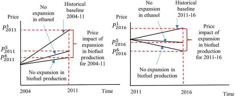
FIGURE 3. A schematic representation of historical baselines and counterfactual experiments including: No expansion in ethanol and No expansion in biofuels. The left panel represents 2004–11 and the right panel illustrates 2011–16. The vertical axis shows the price of a representative product. P¹, P⁵, and P⁶ show the projected prices of this product for the historical baselines, No expansion in ethanol and No expansion in biofuels, respectively.

For the PE simulations we followed the same principle as well. First, we developed a baseline to replicate annual changes in the US markets for gasoline, ethanol, biodiesel, corn, and soybeans and their trade. To accomplish this task, we first calibrated the model to represent actual observations for 2015. We then run the model annually for a set of exogenous variables (e.g., crude oil price, ethanol trade, and targets for biofuel production) and tuning parameters to trace annual changes that occurred in the energy and agricultural markets. Then for each year we developed a counterfactual experiment to evaluate changes in the energy and commodity markets without targeting ethanol production. Hence, for the PE model we have only two cases: A historical annual baseline and a market counterfactual case which does not target production of ethanol. This counterfactual is in line with the CGE counterfactual I.

Shift Factors and Collected Data

The shift factors were determined using an iterative approach between the CGE and PE models and model parameters. We first run the CGE model for 2004–11 and 2011–16 with no shift factors. We learned that for both time periods the model needs shift factors to accurately represent crude oil markets. Using actual observations, we defined shift factors to replicate changes in the crude oil price exogenously. The shift factors indeed capture changes in the global market for crude oil that economic models fail to capture. One example is production of crude oil from shale resources in the US, which altered the global market for this product. When we ran the PE model for annual changes, we found demand shifters are required to properly capture the observed changes in this variable. First, there was the recession, which caused a major downward shift in gasoline demand. Then, the fuel economy standards began to take hold, which also caused a downward shift in gasoline demand. In fact, US gasoline demand did not catch up with the 2007 level until 2016. We developed shifters to represent these exogenous changes in gasoline demand. These shifters developed for the PE model also helped us to calibrate shifters in the gasoline market for the GE model.

In modeling the annual changes in the US markets for corn and soybeans, it became apparent that there were some exogenous shifts in international trade that could not be captured in the standard model and its imbedded parameters. The best example is the very large increase in Chinese imports of soybeans, which was mainly due to policy changes that are not captured in the model. To take care of these changes we included demand shifters to represent changes in the global demand for these products.

To support simulations, data on macro variables including GDP, population, labor force, investment, and GDP deflator were collected from the World Bank data base. A summary of macro variables is presented in Supplementary Table S3.

The GTAP database has data on crop production and harvested area by crop for 2004 and 2011. We prepared the same data for 2016 using data from the Food and Agricultural Organization (FAO) of the United Nations. Supplementary Table S4 provides a summary of crop production and harvested area for the US and the rest of the world for 2004, 2011, and 2016. While the model traces all crop categories included in the data bases, for this table we aggregated crops into three main categories including coarse grains (covering all coarse grains except sorghum), soybeans, and all other crops. Sorghum is included in the other category. The category of coarse grains basically represents corn. In addition to these data items, we collected a wide range of monthly and annual data on crop prices; prices of crude oil, gasoline, and ethanol; trade of agricultural products; etc. to support our analyses and/or to be use in our simulations or to be compared to our results.

Results

Computable General Equilibrium Model Results

As mentioned, we developed a historical baseline and several counterfactual experiments for each time period of 2004–11 and 2011–16. In this section we highlight the following results for each time period:

1) Impacts of removing RFS only for corn ethanol: The difference between the results of RFS baseline and ethanol free of mandate,

2) Impacts of removing RFS for corn ethanol and biodiesel: The difference between the results of RFS baseline and No RFS,

3) Impacts of no expansion in corn ethanol: The difference between the results of Historical baseline and No expansion in ethanol,

4) Impacts of no expansion in biofuels: The difference between the results of Historical baseline and No expansion in biofuels.

Before presenting the results of these experiments, as a measure of validation, we compare the results of the historical simulations on the US crop prices for the time periods of 2004–11 and 2011–16 with their corresponding actual observations in Figure 4. This figure represents changes in crop prices in real terms. Given that GTAP represents real prices, the GDP price deflator is used to convert nominal observed prices to real prices. The left panel of this figure shows that crop prices have increased sharply between 2004 and 2011. This panel also shows that the model projections are in general very close to the actual observations. For this time period, there were somewhat greater differences between the actual observations and model simulations for wheat and rice. The right panel of Figure 5 shows that, unlike the first time period, crop prices have declined largely during the time period of 2011–16. This panel also shows that the model projections are in general very close to the actual observations. For this time period, there was only somewhat greater difference between the actual observation and model simulation for wheat. Hence, in general, the model projections for changes in crop prices are fairly in line with actual observations.

FIGURE 4

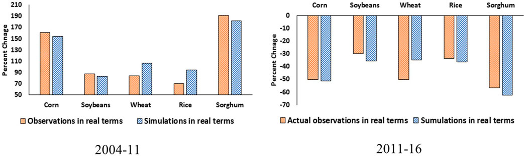
FIGURE 4. Observed and simulated percent change in real crop prices for time periods of 2004–11 (left panel) and 2011–16 (right panel) The GDP price deflator is used to convert nominal prices to real prices.

FIGURE 5

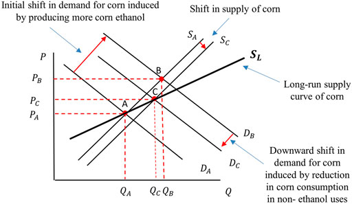
FIGURE 5. Short-run and long-run changes in corn market. This figure was designed to explain difference between the short- and long-run supply elasticities. The demand and supply curves and their shifts are all hypothetical. Box 1 shows numerical estimates.

Results for 2004–2011 Time Period

The mandated level of ethanol for 2011 is 12.6 BG. When we remove this mandate, the market determines consumption of ethanol, and it falls to about 12 BG in 2011. This means that the RFS on ethanol basically boosts consumption of ethanol by about 0.6 BG at the end of the first time period. This can be considered as an additional gradual increase in ethanol consumption by 0.6 BG over the period of 2004–2011. This projection is consistent with findings of the existing literature that non-RFS drivers including higher crude oil prices, tax incentives, added demand for oxygen and octane, and banning consumption of MTBE pave the way for ethanol industry to grow during this time period. In the PE section results, we will explain that in each year of this period, in general, the RFS was not binding except for short periods in 2008 and 2011.

The removal of biodiesel mandate drops consumption of ethanol furthermore by 0.1 BG (from 0.6 BG to 0.7 BG) in 2011. Interactions between livestock, biofuel, and crop industries induced by changes in relative prices cause this tiny reduction. Removing biodiesel mandate reduces production of oilseed meals (by-products of biodiesel) used by the livestock industry. The reduction in meal availability increases production costs of the livestock industry. In response, this industry mainly produces less. This reduction weakens demand for animal feeds (in particular corn and DDGS). This has two opposite effects on profitability of the ethanol industry. The reduction in demand for DDGS drops its price and negatively affects profitability of corn ethanol. On the other hand, fewer demand for corn (as animal feed) reduces corn price which increases profitability of corn ethanol. The net of these two effects combined with changes in the relative prices of gasoline and ethanol, not in favor of ethanol, drops profitability of corn ethanol. This drops ethanol consumption by the tiny amount of 0.1 BG. Note that other factors such as changes in trade of crops and livestock products are also marginally contribute to this observation. These analyses suggest that the biodiesel mandate may have had a minor positive impact on corn ethanol expansion in this time period.

We now analyze the impacts of RFS on commodity outputs and prices. First consider the impacts on commodity outputs presented in the first two numerical columns of Table 1. The first numerical column is for removing ethanol mandate, and the second one is for removing both ethanol and biodiesel mandates. The results show if there was no mandate on ethanol, farmers within the US produce less coarse grains (basically corn) by 1.2% and slightly more of other crops. When we remove both mandates on ethanol and biodiesel, outputs of coarse grains, soybeans, rapeseed, and other oilseeds drop by 1.4, 1.6, 12.4, and 4.3% while outputs of all other crop categories grow slightly. From these results we can conclude, ignoring the contributions of non-RFS factors, the impact of RFS on crop production was very small. However, it encouraged farmers to produce more corn and oilseeds. Later in this section we discuss the overall impacts of biofuel production due to all drivers that encouraged biofuel production.

TABLE 1

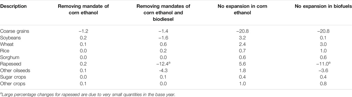
TABLE 1. Percentage change in crop outputs under alternative examined counterfactual experiments for 2004–2011.

Regarding the commodity price impacts of RFS, consider the first two numerical columns of Table 2. The first numerical column is for removing ethanol mandate and the second one is for removing both ethanol and biodiesel mandates. The results show minor impacts in each case and for each crop category. For example, removing ethanol mandate lowers the price of coarse grains and soybeans by 0.3 and 0.1%. When we remove both mandates then these prices fall by 0.6 and 0.7%. The price impacts are also small for all other crop categories.

TABLE 2

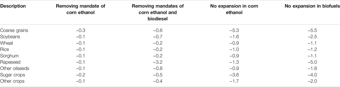
TABLE 2. Percentage change in real commodity prices under alternative counterfactual experiments for 2004–2011.

Now consider the overall impacts of biofuel production due to all drivers that encouraged producing more biofuels. The impacts on commodity outputs are presented in the last two columns of Table 1. The results show that if there was no expansion in ethanol farmers produce less coarse grains (basically corn) by 20.8% and more of all other crops. With no expansion in ethanol and no expansion in biodiesel, regardless of the drivers, outputs of coarse grains, rapeseed, and other oilseeds drop by 20.8, 11, and 3.6% while outputs of all other crop categories grow slightly. From these results we can conclude that biofuel production encouraged farmers to shift to produce more coarse grains (corn) and oilseeds. The impact for corn was large for the first time period. This is consistent with actual objections that confirm changes in the mix of crops produced in the first time period in favor of corn.

Regarding the commodity price impacts of biofuel production consider the last two columns of Table 2. The results show a reduction of 5.3% in the price of coarse grains with no expansion in corn ethanol. The price of coarse grains declines by 5.5% with no expansion in corn ethanol and no expansion in biodiesel.

Results of the CGE modeling practice for the first time period indicate that, in general, the RFS had minor impacts on crop prices. However, the price impacts of the expansion in biofuels were noticeable. For example, our analysis indicates that if there was no expansion in corn ethanol in this time period, supply of corn was lower by 20.8% and price of corn was lower by 5.3%. That means that the expansion in corn ethanol in this time period caused a 20.8% increase in supply of corn ethanol with 5.3% increase in the price of this commodity. A 20.8% increase in supply for 5.3% increase in price represents a relatively elastic supply of corn. In what follows we further explain this outcome.

Consider Figure 5, which demonstrates schematic short-run and long-run analyses for corn market. At the status quo, the market operates at point A, with corn price of P_A and quantity of Q_A. The initial supply and demand curves are presented by S_A and D_A, respectively. An increase in corn ethanol, in the short-run shifts the demand for corn to D_B. With the initial supply curve (S_A) and the new demand (D_B) one may think that the market would move to point B with the higher price of P_B and production of Q_B. However, that would not happen in the real world as market mediated responses begin to act. First, the demand for corn in non-ethanol uses will drop due to higher prices, and that shifts the overall demand for corn downward to D_C. Then the supply of corn will increase over time in response to higher corn prices. Therefore, the supply curve of corn shifts to S_C. With these changes, the market moves to a new equilibrium at point C with supply of Q_C and price of P_C. Clearly, the price of P_C is considerably lower than the price P_B. Figure 5 clearly indicates that, in long-run, the economy moves from point A to C on its long-run supply curve (the bold and back curve of S_L), not on the short-run supply curve of S_A. From Figure 5, one can see that the short run supply curves of S_A and S_C are both less elastic than the long-run supply curve of S_L. In fact, the long-run market mediated responses spread out the price impacts of ethanol production from one crop (i.e., corn) to all crops and by that they mitigate the price impacts for corn. As shown in Tables 5, 6, under all cases, production of corn ethanol affects supplies for all crop categories and their prices. Of course, the extent and intensity of changes vary by crop.

We now explain the implications for food prices. Of course, changes in commodity prices do not translate directly to changes in food prices. When the ethanol RFS or both ethanol and biodiesel requirements were removed, the food price index fell by 0.04%. In other words, the RFS was responsible for only tiny changes in the overall food price index. When ethanol expansion was not permitted, the food price index dropped 0.21%, and when both ethanol and biodiesel expansion was prohibited, the drop was 0.25%. Biofuels did have some small impact on food prices, but not the RFS.

The other important factor to consider is changes in farm income. Farm incomes include the value added generated by crop producers (all king of crops), livestock producers (dairy, ruminant, and non-ruminant farms) and forestry. Value added measures payments to the primary inputs such as land, labor, and capital. The quantity of each primary input times its rental rate represents the value added of that input. For example, value added of labor in corn production equals number of labors (all kinds including management) times the average wage. The GTAP data base includes information on all elements of value added by sectors. The GTP-BIO model traces changes in value added by sector and by the type of primary input. For example, a reduction in mandate on corn ethanol could reduce both area of corn land and the rent rate of land used in corm production. The model determines these changes endogenously. These are shown for the time period 2004–2011 Table 3. First consider the impacts on farmers who produce crops. Removing ethanol mandates decreases incomes of farmers by $461.6 million and removing both mandates on corn ethanol and biodiesel lowers farmers’ incomes by $1,299.6 million for the period of 2004–11. These figures confirm that the RFS had positive impacts on farmer’s incomes. Table 3 also indicates that removing the expansion in corn ethanol drops the farmers’ incomes by $6,923.8 million. The drop in incomes increases to $8,010.6 million with no expansion of either ethanol or biodiesel. These figures confirm that biofuel production had significant favorable impacts on farmers’ incomes during the first time period.

TABLE 3

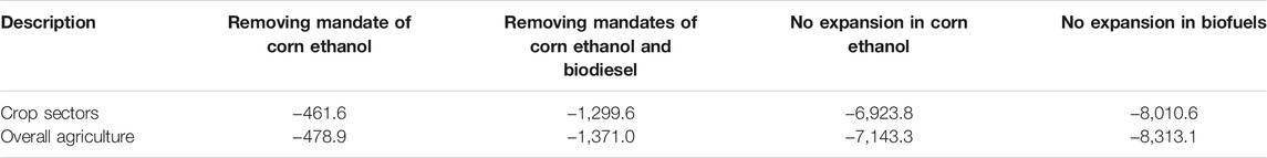
TABLE 3. Changes in farm income with and without the RFS and biofuel changes for 2004–2011 (Million USD).

The last row of Table 3 shows the overall impacts on incomes of the agricultural sectors, including incomes of crop and livestock producers plus incomes of the forestry sector. This row shows slightly larger impacts (in absolute terms) compared with the first row. That confirms that agricultural activities in general gained from the RFS and also biofuel producers. The additional farm incomes are attributed to two factors: 1) slightly higher crop prices and higher land rents induced by biofuel production and 2) retaining and allocating agricultural resources (say land) in higher valued activities. Compared to the baseline, with no expansion in biofuels, nearly 2,563 thousand hectares (6.3 million acres) of the US cropland would go out of production in the time period of 2004–11. The model assigns 16% of these areas to the RFS. In the absence of biofuel production and policy, agricultural production activities would have provided fewer employment opportunities resulted in idled agriculture production capacity and unused resources across rural areas.

Results for 2011–2016 Time Period

Conditions were quite different for the 2011–16 period than for the 2004–11 period. The earlier period was one of rapid growth in ethanol production driven primarily by increasing crude oil prices, the ethanol tax incentives, and changes in the use of ethanol as a source of oxygen and octane in blended fuels. The government’s ethanol support ended in 2011. Ethanol’s role in the gasoline fuel system as an important source of oxygen and octane had been established and continued through the second period and to today. In addition, in the second time period the price of crude oil declined sharply and that caused a sharp reduction in the price of conventional gasoline and a faster reduction in biofuel prices. These factors drove down profitability of ethanol production in the second time period significantly. On the other hand, the RFS targets for the first generation of biofuels (in particular for conventional ethanol) approached their higher required values.

Finally, it is important to take into account that the rate of ethanol blended with gasoline has increased rapidly from about 2.5% in 2004 to nearly 9.6% in 2011 and then continued to increase slowly to 10%. That suggests that in the second time period demand for ethanol basically continued to grow slowly to meet the adjusted down RFS quantities determined and set by the EPA, perhaps based on the traditional 10% maximum ethanol content. As mentioned before, in response to the observed high RIN prices, which could reflect constraints on the growth in consumption of ethanol, the EPA adjusted down the original enacted RFS targets for 2014–2016. The effective mandated level of ethanol for 2016 was 14.3 BG⁵. When we remove this level of mandate, the market forces drop the consumption of ethanol to 12.5 BG. This means that the RFS on ethanol basically boosts consumption of ethanol by about 1.8 BG for the second time period. This means that the mandate on corn ethanol was more important in the second time period. In the PE section results, we will explain annual contributions of the RFS to consumption of ethanol.

The removal of biodiesel mandate eliminates a portion of the reduction in ethanol consumption by 0.3 BG. Hence, removing both ethanol and biodiesel mandates drops consumption of ethanol by 1.5 BG. This means removing biodiesel mandate increases ethanol consumption for the period 2011–16. In this period the removal of biodiesel mandate drops consumption of this biofuel by a relatively a large quantity of 1.2 BG, which confirms that the RFS is very effective in 2011–16. Similar to the case of 2004–11, removing biodiesel mandate reduces production of oilseed meals (by-products of biodiesel) used by the livestock industry. The reduction in meal availability increases production costs of the livestock industry. However, for the time period of 2011–16, due to a stronger demand for meat products, the livestock industry instead of cutting supply uses other feeds including other feed crops and DDGS to replace the missing meals. The higher demand for DDGS plus a lower corn price due to conversion of cropland from oilseeds to corn improve profitability of corn ethanol. This leads to an increase in corn ethanol supply and consumption by about 0.3 billion gallons.

We now analyze the impacts of RFS on commodity outputs and prices. First, we consider the impacts on commodity outputs presented in the first two numerical columns of Table 4. The first numerical column is for removing the ethanol mandate, and the second one is for removing both ethanol and biodiesel mandates. The results show if there was no mandate on ethanol, farmers would produce 2% less coarse grains (basically corn) and slightly more of other crops. This percent reduction in absolute terms is larger than the corresponding figure for the first time period. One needs to take into account the fact that the base of consumption in the second time period is also larger than the base of consumption in the first time period⁶. When we remove both mandates on ethanol and biodiesel, outputs of coarse grains drop by 1.6% and again supplies of other crops increase slightly.

TABLE 4

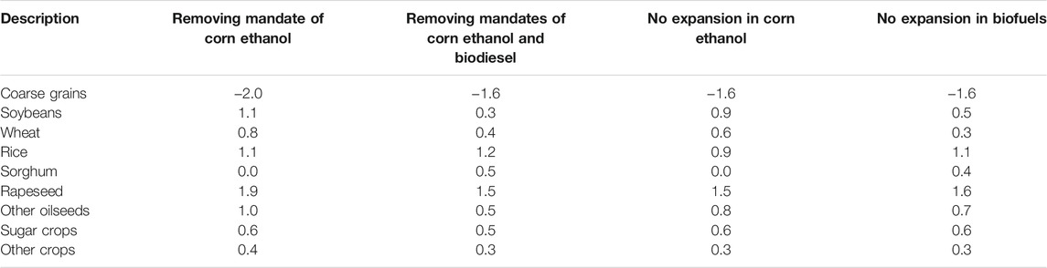
TABLE 4. Percentage change in crop outputs under alternative examined counterfactual experiments for 2011–2016.

For the period of 2011–16, unlike the first period of 2004–11, removing the expansion in corn ethanol alone (or jointly with biodiesel) has much smaller impacts on crop supplies. Compare the last two columns of Table 4 and with their corresponding columns of Table 1. In the second time period, production of corn ethanol did not grow substantially. It only changed from 13.9 BG in 2011 to 15.4 BG in 2016, an increase of 1.5 BG.

Regarding the commodity price impacts of RFS in the second time period, consider the first two numerical columns of Table 5. The first numerical column is for removing the ethanol mandate and the second one is for removing both ethanol and biodiesel mandates. Similar to the first time period, the results show that in the second time period the price impacts of removing the RFS requirements (for only corn ethanol or both biofuels) are small, less than 1%. Nonetheless, the RFS price impacts are larger in the second time period. Unlike the first time period, the RFS was the key driver of the expansion in biofuels in the second time period. Note that, unlike the first time period, removing the expansion in corn ethanol alone (or jointly with biodiesel) in the second time period has no large impacts on crop prices, compare the last two columns of Tables 2, 5. That is because, as mentioned before, in the second time period production of corn ethanol did not grow that much.

TABLE 5

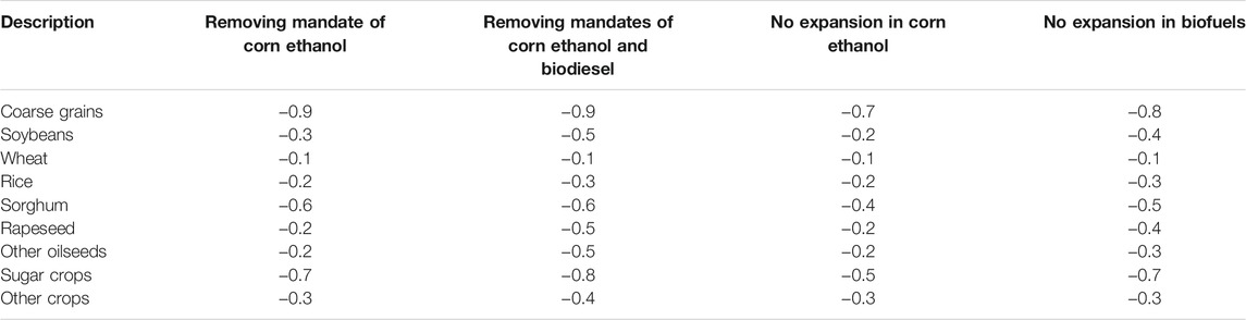
TABLE 5. Percentage change in real commodity prices under alternative counterfactual experiments for 2011–2016.

Finally, we present changes in farm incomes for the time period of 2011–16. Table 6 shows these changes. The first row of this table indicates that, for this time period, removing ethanol mandates drops incomes of farmers by $2,062.2 million, and removing both mandates on corn ethanol and biodiesel drops farmers’ incomes by $2,454.8 million. These figures confirm that the RFS had positive and important impacts on farmer’s incomes in 2011–2016. Table 10 also indicates that removing the expansion in corn ethanol drops the farmers’ incomes by $1,652.2 million. The drop in incomes increases to $2,281.2 million with no expansion of either ethanol or biodiesel. These figures confirm that biofuel production had significant impacts on farmers’ incomes during the second time period as well. The last row of Table 6 shows the overall impacts on incomes of agricultural sectors, including incomes of crop and livestock producers plus incomes of the forestry sector. This row shows slightly different impacts (in absolute terms) compared with the first row.

TABLE 6

TABLE 6. Changes in farm income with and without the RFS and biofuel changes for 2011–16 (Million USD).

Compared to the baseline, with no expansion in biofuels, about 77 thousand hectares (160 thousand acres) of the US cropland would go out of production in the time period of 2011–16. The model assigns 100% of these areas to the RFS. Similar to the first time period, in the absence of biofuel production and policy, agricultural production activities would have provided fewer employment opportunities resulted in idled agriculture production capacity and unused resources across rural areas.

BOX 1 | Long-run analysis versus short-run analysis

In presenting the results for the first time period we explained why a large change in supply of corn in the long-run induces a relatively moderate change in the corn price (see Figure 5 and its corresponding analysis). We showed that the long-run supply of corn is more elastic than its short-run supply. That analysis applies to the second time period as well. For example, removing the ethanol mandate alone reduces supply of corn ethanol by 1.5 BG which causes a reduction in supply of coarse grains (basically corn) by 2%, and that leads to 0.9% reduction in the price. This represents a relatively elastic long-run supply curve. Here we show that in the short-run when demand and supply functions operate with lower elasticities, and markets have limited capacities to respond to the economic shocks, the price impacts could be larger.

To depict the short-run impacts, we repeated the experiment that drops the mandates for ethanol and biodiesel with an inelastic supply for corn, lower substitution between corn and DDGs, and a lower trade elasticity for corn. With these short-term elasticities, the drop in the price of coarse grains changed from -0.9% to -6.7%. We then kept the low trade elasticity and the low substitution between corn and DDGS and allowed the supply of corn to respond. In this case the price of corn changed by -2.7%.

Partial Equilibrium Model Results

The partial equilibrium model described above (AEPE) was used to simulate the annual changes from 2005 to 2016. The model was calibrated to 2005. For the simulations, corn and soybean yields were targeted as in the CGE model. Total area of corn and soybeans (not individually) was also targeted. So, the model allocates land between corn and soybeans. Throughout the period, crude oil price was exogenous as explained above. The net trade of ethanol is exogenous in the PE model. The gasoline consumption was tuned to actual values via shifters. By using demand shifters, we attempted to capture drivers like the 2006 MTBE substitution and the later use of ethanol as an octane additive for blended gasoline. Of course, we also captured the 2012 drought and other agricultural commodity supply and demand changes due to changes in world market conditions. Following the CGE approach, we first developed a historical baseline. However, unlike the CGE work, the PE baseline covers annual changes for each year from 2005 to 2016. Then we made market based annual simulations that only take into account market forces to determine production and consumption of ethanol. Finally, it is important to note that, unlike the CGE model, the PE model uses nominal prices. Hence, the prices presented below are nominal values.

In what follows we present the results for the market-based simulations and compare them with actual observations. We begin with consumption of ethanol. The actual observations and simulated market-based results for ethanol consumption are presented in Figure 6. This figure indicates that prior to 2011 the market-based projections for ethanol consumption were usually slightly larger than their real-world observations, with one exception in 2008. That suggests a non-binding RFS prior to 2011, except for 2008. Since 2011 the market-based projections for ethanol consumption were smaller than their real-world observations. That means the RFS pushed up consumption of ethanol in these years. For example, in 2016 the actual consumption of ethanol was 14.3 BG with a market-based projection of 12.1 BG. This means that in this particular year the RFS increased consumption of ethanol by about 2.1 BG. This is the largest contribution of RFS to ethanol consumption over our study period. These results are consistent with our CGE findings.

FIGURE 6

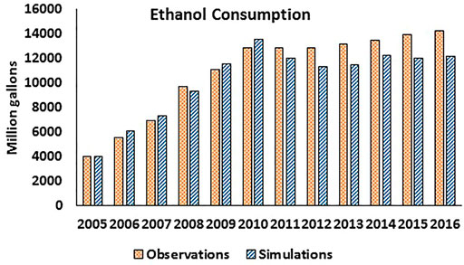
FIGURE 6. Actual and simulated market results for ethanol consumption 2005–16.

The actual observations and simulated market-based results for corn and soybean prices are presented in Figure 7. This figure shows that, in general, the actual observations and market-based projections are similar with some noticeable exceptions. For example, in 2016 the actual corn price was $3.33 per bushel with a market-based projection of $3.16 per bushel, 5% lower than the actual observation. From 2005 to 2009 the market-based projections for the price of corn were higher than the baseline, and then the reverse occurred.

FIGURE 7

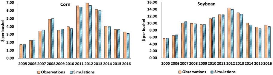
FIGURE 7. Observed and simulated market results for corn and soybean nominal prices 2005–16.

The actual observations and simulated market-based results for ethanol and gasoline prices are presented in Figure 8. This figure shows that, from 2005 to 2010 the market-based projections for ethanol price are higher than the actual observations, except in 2008. Then from 2011 the reverse has happened. For example, the actual ethanol price in 2016 was $1.43 per gallon with a market-based projection of $1.20 per gallon. Hence one can conclude that since 2011 the RFS has positively affected the price of ethanol.

FIGURE 8

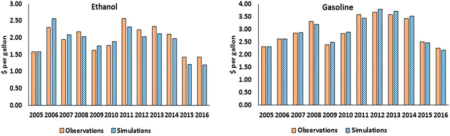
FIGURE 8. Observed and simulated market results for ethanol and gasoline nominal prices 2005–16.

Conclusion

Determining the economic impacts of the RFS is a complicated task. Part of the complication is the questions of attribution. For example, some of the early literature tended to blame the RFS for all increases in commodity prices. However, over time it has become abundantly clear that many factors have been involved in the evolution of commodity and food prices, with the RFS and biofuel production in general being only one. The purpose of this study is to determine the extent to which commodity and food prices were driven by the RFS and to what extent they were driven by biofuels regardless of what caused the level of biofuels production.

This study first examines the literature and data on what was actually happening in agricultural and energy markets over the relevant period. From the data presentation and literature review alone, it became clear that the bulk of the ethanol production prior to 2012 was driven by what was happening in the national and global markets for energy and agricultural commodities and by the federal and sometimes state incentives for biofuel production. This conclusion is supported by examining the data, by the conclusions of the recent literature, and by the fact that until 2012 the RINs prices were very low, indicating that the non-RFS policies and market forces (demand for ethanol as a fuel extender, demand for ethanol as an additive, and MTBE ban) helped biofuels to grow, while the RFS provided a safety net for the whole biofuel industry to invest and expand its production capacity by requiring minimum levels of biofuels use.

We provided long-run CGE analyses for two time periods: 2004–2011 and 2011–2016. Our results confirm that, in general, the long-run price impacts of biofuel production were not large. Due to biofuel production, regardless of the drivers, crop prices (adjusted to inflation) have increased between 1.1% (for wheat) and 5.5% (for the category of coarse grains) in the first time period (i.e., 2004–11). The model determines the contributions of RFS to the price increases due to biofuel production. For example, as shown in Table 1, the model results indicate that the price of coarse grains drops by 5.5% with no expansion in biofuels compared to baseline. On the other hand, the price of coarse grains drops by 0.6% with no mandates compare to the corresponding baseline. Therefore, only one-tenth of the 5.5% increase in the price of coarse grains is related to the RFS impacts. For the second time period (i.e., 2011–16) the long-run price impacts of biofuels were less than the first time period, as in this period biofuel production has increased slowly. Due to biofuel production, crop prices have increased by less than 1% in the second time period. However, unlike the first time period, the RFS was the main driver of these changes. Finally, in both time periods, the long-run effects of biofuel production and policy on food prices were negligible for both time periods.

The long-run CGE results indicate that biofuel production and policy made major contributions to the agricultural sector in both time periods, while they only affected the commodity prices moderately. Biofuel production, regardless of the drivers, has increased the US annual farm incomes by $8.3 billion and $2.3 billion at constant prices in the first and second time periods, respectively. Hence, with no biofuels, the US annual farm income would drop by an estimated $10.6 billion, ignoring the changes since 2016. The model assigns 28% of the expansion in farm incomes of the first time period to the RFS. The corresponding figure for the second time period is 100%. This means that, the additional gains in farm incomes were entirely due to the RFS in the second time period. As explained with details in the results section, for the second time period (2011–2016), when we remove mandates the uses of biofuels decline almost to their initial levels in 2011 or even lower for the cases of biodiesel. Hence, the reduction in farm incomes caused by the removal of mandates is entirely due to the RFS effect in the second time period.

The PE analyses indicate that prior to 2011 the market-based projections for annual consumption of ethanol are usually smaller than their real-world observations, with one exception in 2008. That suggests a binding RFS in this year. Since 2011 the market-based projections for annual ethanol consumption are smaller than their real-world observations. That means the RFS pushed up consumption of ethanol in these years. The RFS has increased the demand for ethanol by 7–14% between 2011 and 2016. For example, in 2016 the actual consumption of ethanol was 14.3 BG with a market-based projection of 12.1 BG. This means that in this particular year the RFS increased consumption of ethanol by about 2.1 BG. The impact of RFS on the price of corn in this year was about 5%.

Prior to 2011, ethanol was basically in demand as a fuel extender and an octane additive. This has changed after this year and a portion of ethanol was consumed as a source of octane and as a substitute for gasoline to meet the RFS requirements. Since 2011 as the total consumption of ethanol moved towards the historical 10% maximum ethanol content (that was allowed in non-flex-fuel vehicles), demand for gasoline, and hence, ethanol did not grow enough and that raised the RINs prices. This could change in the future considering that E15 has been approved for use in 2001 and newer vehicles since 2011 and flex-fuel vehicles using E85. The USDA’s 2015 Biofuels Infrastructure Partnership, in combination with private-sector resources, has helped improve market access for higher blends of ethanol. The more recent evidence confirms that the consumption of ethanol has passed the historical 10% bend rate and demand for E15 and E85 is growing since 2016. Since our analyses end in 2016, this paper does not cover these new developments.

There is clearly a difference in impacts of the RFS and biofuels production due to market forces. One of the main contributions of this research is to demonstrate that biofuels production growth that is often attributed to the RFS is actually due to energy and agricultural market conditions and key drivers. We have identified and characterized these drivers and shown that the market drivers have been the main contributor to biofuels growth, in particular through 2011. In a sense, this means that biofuels’ contribution to commodity price increases is really no different from fructose corn syrup, increased feed demands, or other market demands. Indeed, they all affect commodity price through the same mechanism. To understand what has happened to agricultural markets over the past 2 decades, it is absolutely critical to include in the analysis all the global and national demand and supply factors in both energy and agricultural markets, and we have done that.

An interesting question to ask given our conclusions on the role of markets in driving biofuels growth is how it would have been different if all these market changes had not occurred. In other words, what if crude oil price had not surged, MTBE had not been banned, ethanol did not get integrated into the fuel system becoming a fuel additive instead of a fuel extender, etc.? The answer is clearly that the RFS would have played a much greater role. So, in a sense, the RFS has been the backstop, but by circumstance, it was overpowered by tax incentives and market forces prior to 2011.

Another interesting comparison is between what happened over this period for ethanol compared with biodiesel and cellulosic biofuels. For both biodiesel and cellulosic biofuels, the original mandated levels have not been implemented in practice and frequently revised over time. Hence, the RFS has not reached its original goals for these biofuels. However, after the waivers, the RFS was still clearly an important driver of production and consumption. RIN prices were always relatively high, and the RFS was always binding for biodiesel and cellulosic ethanol. Clearly, the market changes that benefitted ethanol did not work as much in favor of these other biofuels.

These findings could help policy makers to define the goals of the RFS beyond the year of 2022, as this policy only specified targets for consumption of biofuels until 2022. In defining the future goals of this policy, it is important to evaluate the potential new sources of demand for biofuels. While demand for biofuels in road transportation may not grow significantly in future, the use of biofuels in aviation industry could play an important role in defining the future goals for the RFS. The International Civil Aviation Organization (ICAO) of the United Nations has defined the Carbon Offsetting and Reduction Scheme for International Aviation (CORSIA) to reduce Greenhouse Gas (GHG) emissions. Sustainable Aviation Fuels (SAFs) will play an important role in achieving the goal of this scheme (Zhao et al., 2021; Prussi et al., 2021: in press). An explicit recognition of these biofuels by the RFS will help the biofuel industry to operate in a secure environment in future.

Data Availability Statement

The original contributions presented in the study are included in the article/Supplementary Material, further inquiries can be directed to the corresponding author.

Author Contributions

Conceptualization: FT, WT, HB; Methodology FT, WT; Data Assembly: FT; Simulations: FT; Formal Analysis: FT, WT, HB; Original Draft: WT, FT; Final Draft: FT, HB. Virtualizations: FT; Supervision: FT, WT.

Funding

This study received financial support from: National Corn Growers Association and the Renewable Fuels Association.

Conflict of Interest

The authors declare that the research was conducted in the absence of any commercial or financial relationships that could be construed as a potential conflict of interest.

Publisher’s Note

All claims expressed in this article are solely those of the authors and do not necessarily represent those of their affiliated organizations, or those of the publisher, the editors and the reviewers. Any product that may be evaluated in this article, or claim that may be made by its manufacturer, is not guaranteed or endorsed by the publisher.

Acknowledgments

The content of this manuscript has been partly presented at the following conferences: 23rd Annual Conference on Global Economic Analysis, June 2019, Virtual; Agricultural and Applied Economics Association Meeting, July 2019, Virtual; and European Association of Agricultural Economics Meeting, July 2021, Virtual.

Supplementary Material

The Supplementary Material for this article can be found online at: https://www.frontiersin.org/articles/10.3389/fenrg.2022.749738/full#supplementary-material

Footnotes

¹The form and amount of the government support has changed over the years.

²Yao et al. (2018) have followed this approach and developed a static historical baseline for the time period of 2004–11 for a different application. For details see the appendix of the paper.

³The standard GTAP model endogenously determines GDP for given changes in primary factors of production and TFP. In the baseline simulation we shock the model for the observed changes in GDP and primary factors of production. This allows us to alter the model closure to determine TFP for the given changes in GDP and primary factors of production. This is a standard approach for estimating TFP by country using a CGE model.

⁴The Standard GTAP model uses production functions to determine crop supplies. The production function of each crop determines supply of that crop for given inputs (including intermediate and primary inputs) and rates of unbiased and biased technological progress. The rate of unbiased technological progress for each crop acts as a shift factor in the supply function of that crop. In our baseline simulation we will ask the model to determine these crop specific shift factors for the observed changes in crop supplies.

⁵This was indeed very close to 10% of gasoline consumption in this year.

⁶Note that for the first time period, the comparison is for supplies of corn with and without mandate in 2011. For the second time period, the comparison is for supplies of corn with and without mandate in 2016.

References

Abbott, P. (2014). “Biofuels, Binding Constraints, and Agricultural Commodity price Volatility,” in The Ecnomics of Food Volatility. Editors J. Chavas, D. Hummels, and B. D. Wright (Chicago, Illinois, USA: University of Chicago Press), 91–134.

Google Scholar

Abbott, P., Hurt, C., and Tyner, W. E. (2011). What's Driving Food Prices in 2011?, in Issue Report 2011, Farm Foundation. Issue Report. Avialble at: What’s Driving Food Prices in 2011? (repec.Org).

Google Scholar

Abbott, P., Hurt, C., and Tyner, W. E. (2009). What's Driving Food Prices? Farm Foundation, Issue Report. Available at: What's Driving Food Prices? March 2009 Update (repec.Org).

Google Scholar

Abbott, P., Hurt, C., and Tyner, W. E. (2008). What’s Driving Food Prices? Farm Foundation, Issue Report, Available at: What's Driving Food Prices? (repec.Org).

Google Scholar

Agricultural Marketing Resource Center (2019). Ethanol Profitability. Ames, Iowa: Agricultural Marketing Resource Center, Iowa State University. Available at: http://www.agmrc.org/renewable_energy/.

Google Scholar

Beckman, J., Hertel, T., Taheripour, F., and Tyner, W. (2012). Structural Change in the Biofuels Era. Eur. Rev. Agric. Econ. 39 (1), 137–156. doi:10.1093/erae/jbr041

CrossRef Full Text | Google Scholar

Brookes, G., Taheripour, F., and Tyner, W. E. (2017). The Contribution of Glyphosate to Agriculture and Potential Impact of Restrictions on Use at the Global Level. GM Crops & Food 8 (4), 216–228. doi:10.1080/21645698.2017.1390637

CrossRef Full Text | Google Scholar

Chiou-Wei, S.-Z., Chen, S.-H., and Zhu, Z. (2019). Energy and Agricultural Commodity Markets Interaction: An Analysis of Crude Oil, Natural Gas, Corn, Soybean, and Ethanol Prices. Energ. J. 40 (2), 265–296. doi:10.5547/01956574.40.2.schi

CrossRef Full Text | Google Scholar

Delgado, C. (2008). Food Policy Implications of Longer-Run Price Rise. Washington, D.C., USA: Agriculture and Rural Development Department. World Bank.

Google Scholar

Filip, O., Janda, K., KristoufekZilberman, L. D., and Zilberman, D. (2019). Food versus Fuel: An Updated and Expanded Evidence. Energ. Econ. 82, 152–166. doi:10.1016/j.eneco.2017.10.033

CrossRef Full Text | Google Scholar

Henderson, J. (2008). What Is Driving Food Price Inflation? Kansas City, Missouri, USA: Federal Reserve Bank of Kansas City.

Google Scholar

Hertel, T. W. (1997). Global Trade Analysis: Modeling and Applications. New York: Cambridge University Press.

Google Scholar

Hertel, T. W., Tyner, W. E., and Birur, D. K. (2010). The Global Impacts of Biofuel Mandates. Energ. J. 30 (1), 75–100.

CrossRef Full Text | Google Scholar

Irwin, S. (2019). Revisiting the Value of Ethanol in E10 Gasoline Blends. Illinois: University of Illinois. Farmdoc daily (9):60, Available at: https://farmdocdaily.illinois.edu/2019/04/revisiting-the-value-of-ethanol-in-e10-gasoline-blends.html.

Google Scholar

Korting, C., Gorter, H., and Just, D. R. (2019). Who Will Pay for Increasing Biofuel Mandates? Incidence of the Renewable Fuel Standard Given a Binding Blend Wall. Am. J. Agric. Econ. 101 (2), 492–506. doi:10.1093/ajae/aay047

CrossRef Full Text | Google Scholar

Prussi, M., Lee, U., Wang, M., Malina, R., Valin, V., Taheripour, F., et al. (2021). CORSIA: The First Internationally Adopted Approach to Calculate Life-Cycle GHG Emissions for Aviation Fuels. Renew. Sustain. Energ. Rev.

CrossRef Full Text | Google Scholar

Taheripour, F., Zhao, X., and Tyner, W. E. (2017b). The Impact of Considering Land Intensification and Updated Data on Biofuels Land Use Change and Emissions Estimates. Biotechnol. Biofuels 10 (191), 191. doi:10.1186/s13068-017-0877-y

CrossRef Full Text | Google Scholar

Taheripour, F., Cui, H., and Tyner, W. E. (2017a). “An Exploration of Agricultural Land Use Change at the Intensive and Extensive Margins: Implications for Biofuels Induced Land Use Change,” in Bioenergy and Land Use Change, American Geophysical Union. Editors Z. Qin, U. Mishra, and A. Hastings. (Hoboken, NJ, USA: Wiley)

Google Scholar

Taheripour, F., Fiegel, J., and Tyner, W. (2016a). Development of Corn Stover Biofuel: Impacts on Corn and Soybean Markets and Crop Rotation. Sustain. Agric. Res. 5 (1), 1–9.

Google Scholar

Taheripour, F., Hertel, T. W., and Ramankutty, N. (2019). Market-mediated Responses Confound Policies to Limit Deforestation from Oil palm Expansion in Malaysia and Indonesia. Proc. Natl. Acad. Sci. USA 116 (38), 19193–19199. doi:10.1073/pnas.1903476116

PubMed Abstract | CrossRef Full Text | Google Scholar

Taheripour, F., Mahaffey, H., and Tyner, W. E. (2016b). Evaluation of Economic, Land Use, and Land Use Emission Impacts of Substituting Non-GMO Crops for GMO in the United States. AgBioForum 19 (2), 156–172.

Google Scholar

Taheripour, F., and Tyner, W. (2013). Biofuels and Land Use Change: Applying Recent Evidence to Model Estimates. Appl. Sci. 3, 14–38. doi:10.3390/app3010014

CrossRef Full Text | Google Scholar

Taheripour, F., and Tyner, W. E. (2018). Impacts of Possible Chinese Protection on US Soybeans and Other Agricultural Commodities. Quarter 2.

Google Scholar

Taheripour, F., and Tyner, W. E. (2011). Introducing First and Second Generation Biofuels into GTAP Data Base Version 7 in GTAP. Research Memorandum No 21. West Lafayette, IN, USA: Purdue University.

Google Scholar

Taheripour, F., and Tyner, W. E. (2014). Corn Oil Biofuel Land Use Change Emission Impacts: Sharing Emission Savings between Ethanol and Biodiesel. Biofuels 5 (4), 353–364. doi:10.1080/17597269.2014.977582

CrossRef Full Text | Google Scholar

Taheripour, F., Tyner, W. E., and Sarica, K. (2014). “Shale Gas Boom, Trade and Environmental Policies: Global Economic and Environmental Analyses in a Multidisciplinary Modeling Framework (2014),” in Issues in Environmental Science and Technology, Vol. 39 Fracking. Editors R. E. Hester, and R. Harrison (Cambridge, UK: Royal Society of Chemistry).

Google Scholar

Trostle, R. (2008). Global Agricultural Supply and Demand: Factors Contributing to the Recent Increase in Food Commodity Prices.” Economic Research Service. United State. Department Agric. May 2008.

Google Scholar

Trostle, R., Marti, D., Rosen, S., and Westcott, P. (2011). Why Have Food Commodity Prices Risen Again? Washington, D.C., USA: U.S. Department of Agriculture Economic Research Service, WRS-1103.

Google Scholar

Tyner, W. E. (2012). Biofuels and Agriculture: a Past Perspective and Uncertain Future. Int. J. Sustain. Develop. World Ecol. 19, 389–394. doi:10.1080/13504509.2012.691432

CrossRef Full Text | Google Scholar

Tyner, W. E., Dooley, F., and Viteri, D. (2010a). Alternative Pathways for Fulfilling the RFS Mandate. Am. J. Agric. Econ. 2010 (5), 92. doi:10.1093/ajae/aaq117

CrossRef Full Text | Google Scholar

Tyner, W. E., Taheripour, F., and Perkis, D. (2010b). Comparison of Fixed versus Variable Biofuels Incentives. Energy Policy 38 (10), 5530–5540. doi:10.1016/j.enpol.2010.04.052

CrossRef Full Text | Google Scholar

Tyner, W. E., and Taheripour, F. (2008). Policy Options for Integrated Energy and Agricultural Markets*. Rev. Agric. Econ. 30 (3), 387–396. doi:10.1111/j.1467-9353.2008.00412.x

CrossRef Full Text | Google Scholar

Tyner, W. E. (2008). The US Ethanol and Biofuels Boom: Its Origins, Current Status, and Future Prospects. BioScience 58 (7), 646–653. doi:10.1641/b580718

CrossRef Full Text | Google Scholar

Tyner, W. E., and Viteri, D. (2010). Policy Update: Implications of Blending Limits on the US Ethanol and Biofuels Markets. Biofuels 1 (2), 251–253. doi:10.4155/bfs.09.24

CrossRef Full Text | Google Scholar

U.S. Congress (2004). American Jobs Creation Act of 2004, Public Law 108-357, 108th Congress. Washing D.C: U.S. Congress.

Google Scholar

U.S. Congress (1990). Clean Air Act of 1990, Public Law 101–549. Washing D.C: U.S. Congress.

Google Scholar

U.S. Congress (2007). Energy Independence and Security Act of 2007, in H.R. 6, 110 Congress, 1st Session. Washing D.C: U.S. Congress.

Google Scholar

U.S. Congress (2005). Energy Policy Act of 2005, Public Law 109-58. 2005. Washing D.C: U.S. Congress.

Google Scholar

U.S. Congress (1978). National Energy Conservation Policy Act, Public Law 95-619, 95th Congress (1977-78), H.R. 5037. Washing D.C: U.S. Congress.

Google Scholar

Wright, B. D. (2011). Biofuels and Food Security: Time to Consider Safety Valves? Washington D.C: International Food and Agricultural Trade Policy Council IPC.

Google Scholar

Yao, G., Hertel, T. W., and Taheripour, F. (2018). Economic Drivers of Telecoupling and Terrestrial Carbon Fluxes in the Global Soybean Complex. Glob. Environ. Change 50, 190–200. doi:10.1016/j.gloenvcha.2018.04.005

CrossRef Full Text | Google Scholar

Zhang, Z., Lohr, L., Escalante, C., and Wetzstein, M. (2010). Food versus Fuel: What Do Prices Tell Us? Energy Policy 38 (1), 445–451. doi:10.1016/j.enpol.2009.09.034

CrossRef Full Text | Google Scholar

Zhao, X., Taheripour, F., Malina, R., Staple, M., and Tyner, W. (2021). Estimating Induced Land Use Change Emissions for Sustainable Aviation Biofuel Pathways. Sci. Total Environ. 779, 146238. doi:10.1016/j.scitotenv.2021.146238

PubMed Abstract | CrossRef Full Text | Google Scholar