Tuning Analysis and Optimization of a Cluster-Based Aiming Methodology for Solar Central Receivers

1 Introduction

Concentrating power technologies are confronted with the challenge of improving operational consistency, reducing operational costs, and providing competitive solutions against fossil fuel-based technologies (Papaelias et al., 2018). For solar power tower systems, there exists an additional challenge of assigning an aiming point to each heliostat on a large solar field from a power tower traditionally approached from an optimization perspective, which seeks to minimize spillage under the constraints given by the receiver integrity and actual radiation conditions (Wang et al., 2017; Ashley et al., 2019).

A highly prevalent practice in tower plants for the receiver controller is to regulate the outlet temperature by adjusting the mass flow of the molten salt (Buck and Schwarzbözl, 2018). A solar field controller is used to determine all the aiming points and consequently the setpoints for the local controllers that act upon each heliostat. During transient atmospheric disturbances, heliostats are defocused when needed while increasing the mass flow to protect the receiver. The dynamic performance of a concentrating solar power (CSP) receiver depends on a range of factors such as the mass flow of the molten salt, the aiming strategy, and the available solar radiation. Furthermore, the effect of passing clouds over the solar field has been affirmed as one of the most significant disturbances to the system (Crespi et al., 2018). Such effects impact energy production in addition to the loss of revenue caused by using conservative thermal stress limits (González-Gómez et al., 2021). Therefore, alternative control strategies have been devised to improve the thermal energy intercepted by the receiver by using the solar field to adapt to unstable weather conditions.

A noteworthy advantage of closed-loop control is its ability to compensate for disturbances. Thus, recent studies have endeavored to tackle the aim point search as a closed-loop control problem. These studies have demonstrated that using a heliostat grouping strategy to reduce the dimension of the problem can be advantageous (Acosta et al., 2021) as such grouping has also proven meritorious for optimization (Oberkirsch et al., 2021). Dynamic aiming strategies, which compensate for disturbances in the solar field caused by the stochastic nature of weather conditions, have been of interest in academic literature. For instance, in (García et al., 2018), a feedback-loop aiming strategy, using groups of heliostats, restores the solar receiver to a steady state after transient operations caused by clouds. Recently, in (Speetzen and Richter, 2021), a reduced optimization is formulated as an integer linear programming problem where groups of heliostats are used to accelerate the run-time to compute a solution. In (Wang et al., 2021), an algorithm is proposed to match flux distributions to local values of allowable flux on the receiver through an efficient use of ray-tracing and aiming strategy optimization.

This study was conducted with the objective of devising a dynamic aiming methodology suitable for working under closed-loop control strategies. The proposed method entails an optimization procedure for two tuning parameters, one that limits how far the aiming point of the heliostat can move from the equator line of the receiver $\left(D_{h_{frac}}\right)$, and a second one that represents its direction (upward or downward, $ud$ ), and a parametric study using three different sets of constraints for this optimization. The proposed method can function as a standard control method for solar fields. This paper is organized as follows: Section 2 describes the study methodology, while Section 3 shows the main results and discussion. Finally, Section 4 draws the main conclusions.

2 Methodology

This study is predicated on the results obtained by a series of coupled numerical models and algorithms for representing the performance of a solar power tower. The methodology adopted in this study is systematically illustrated in Figure 1. First, a combined algorithm was created, which comprised an optical model and the aiming methodology linked to an optimization routine through a cost function. The optimization yielded a set of tuning parameters, and the ones that maximized the cost function were recorded. Next, the whole optimization loop was executed using a design scenario. Finally, the performance of the optimal values was tested under several off-design scenarios to derive appropriate conclusions about its possible implementation under different configurations of solar field and receiver.

FIGURE 1

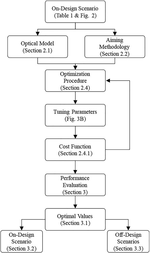
FIGURE 1. The methodology adopted in this study.

2.1 Optical Model of the Heliostat Field and the Central Receiver

In this study, solar radiation interaction with a field of heliostats and its reflection toward the central receiver were investigated (see Figure 2A). The model takes into consideration 1) the position of the Sun, 2) the location of the heliostats in the solar field, 3) the blocking and shading effect, 4) optical properties of the heliostat mirrors, 5) atmospheric conditions, and 6) the target coordinates on the receiver. The model uses a convolution-based method formulated previously (Kiera, 1989; Schwarzbözl et al., 2009). It was chosen as it requires less computing power than its ray-tracing alternatives. This optical model is primarily characterized by the heat flux (HF) calculation presented in Eq. 1 (Schwarzbözl et al., 2009), where $P_H$ is the peak incident power on the image plane over the receiver in Eq. 2, $x$ and $y$ are the coordinates of the receiver at its surface, $x_{ap}$ and $y_{ap}$ represent the points where the aiming point is located, ${\sigma }_{HF}$ is the total effective deviation of the mirror, ${\eta }_{opt}$ is the overall optical efficiency of the solar field, DNI is the direct normal irradiance, and $A_m$ is the total area of the mirrors.

$HF=\frac{P_H}{2\pi {\sigma }_{HF}^2}{e}^{-\frac{{\left(x-x_{ap}\right)}^2+{\left(y-y_{ap}\right)}^2}{2{\sigma }_{HF}^2}}(1)$

$P_H={\eta }_{opt}DNI{A}_m(2)$

FIGURE 2

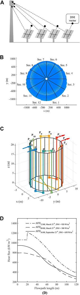
FIGURE 2. (A) Scheme of solar radiation reflected from the heliostat field toward the receiver (B) Solar field layout. Adapted from (Flesch et al., 2017) (C) Flow paths within the studied receiver. The squared marked line represents flow path 1 going from panel 1 through 7 (D) AFD for the studied receiver at different times and days.

This study used the southern hemisphere solar field layout presented by (Flesch et al., 2017). Table 1 and Figure 2B present the primary characteristics of the central receiver used in this study. The central receiver comprises 12 panels, and thus, the solar field is also divided into 12 sections, as shown in Figure 2C. The models were validated in two previous studies (Soo Too et al., 2019; García et al., 2020). The combination of this solar field, receiver, and operating conditions was considered the “on-design scenario,” which is discussed later while elaborating on the performance of the tuning optimization.

TABLE 1

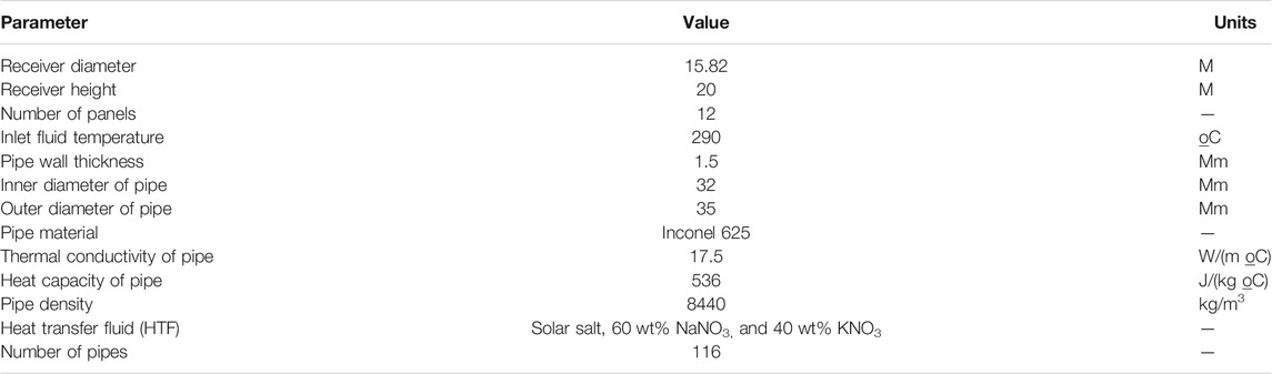
TABLE 1. Main parameters of the central receiver.

The operation of central receivers requires compliance with important constraints. The most noteworthy constraints include the corrosion of the panel tubes and the thermal stresses. Consequently, different studies have developed a single parameter known as the allowable flux density (AFD), which groups both constraints (Vant-Hull, 2002; Liao et al., 2014; Sánchez-González et al., 2016). Accordingly, Figure 2D shows the AFD curves for the selected combination of receiver and solar field at different times of the day and different seasons of the year. These profiles were derived from the methodology presented in (Sánchez-González et al., 2020), in which thermal stress and corrosion constraints in molten-salt receivers are translated into flux limits.

2.2 Aiming Methodology Onto the Receiver

The aiming methodology employed in this paper, proposed in (García et al., 2020), groups the aiming points of the heliostats into several clusters and uses an algorithm based on the working principle of a control valve (see Figure 3A). This methodology allows reducing the degrees of freedom to achieve an appropriate flux distribution, avoid exceeding the AFD, and allow the possibility of using closed-loop control strategies through a wide range of approaches. Figure 3B shows the primary sequence of equations used in the methodology for determining the aiming points of each heliostat. In general, the methodology consists of calculating each aiming point in accordance with its movement ( $\Delta d\left(t\right)$ in Eq. 4) over a predefined path given by values in $X_{path}$, $Y_{path}$, and $Z_{path}$ (see from Eq. 5–7. The methodology begins with the signals $m\left(t\right)$ (one per panel), which represent the valve aperture. These values go to the dynamic representation of the valve in Eq. 3. In Eq. 3, which can be used to find the mean distance of each aiming point within the group and the center of the panel, $a_p\left(t\right)$ is the aperture of the group and goes from 0 to $C_{v_{\max }}$. $C_{v_{\max }}$ represents the maximum mean distance that the group can have, $\alpha$ is the rangeability parameter for equal percentage valves, and $\tau$ is the time constant of the control valve. Vector $a_p\left(t\right)$ represents the average movement of the aiming points within a group. The actual motion of each aiming point (Eq. 4) is adjusted according to the distance of the heliostat to the tower. Thus, the aiming points of the heliostats at a large distance from the tower should not have too much movement. This characteristic is determined by vector $D_{h_{frac}}$, one of the tuning variables used in this study, whose size equals the number of heliostats. Readers are encouraged to check the aiming methodology insights expounded in (García et al., 2020) to understand all the details and variables used in Eq. 4. The second tuning term is vector $ud$, whose purpose is to check if the $Y_{path}$ for each heliostat goes upward or downward from the equator of the receiver. Then, each aiming point gets a binary value, either +1 or −1. Once these two parameters are defined, both are kept constant during the operation of the aiming methodology.

$\frac{1}{\tau }\frac{\mathbf{d}{\mathbf{a}}_p\left(t\right)}{dt}+{\mathbf{a}}_p\left(t\right)=C_{v_{\max }}{\alpha }^{-\frac{\mathbf{m}\left(\mathbf{t}\right)}{100}}(3)$

$\Delta {\mathbf{d}}_{N_h\times 1}\left(t\right)=\mathbf{min}\left\{\left[\mathbf{G}{\mathbf{a}}_p\left(t\right)\right]\odot \left[\overrightarrow{1}-{\mathbf{D}}_{{\mathbf{h}}_{frac}}\right]-\mathbf{\delta }\left(t\right),\mathbf{\Delta }{\mathbf{d}}_{\mathbf{max}}\right\}(4)$

${\mathbf{X}}_{a{p}_{Nh\times 1}}\left(t\right)={\mathbf{X}}_{ap}\left(t-\Delta t\right)+{\mathbf{X}}_{path}\odot \mathbf{\Delta }\mathbf{d}\left(t\right)(5)$

${\mathbf{Y}}_{a{p}_{Nh\times 1}}\left(t\right)={\mathbf{Y}}_{ap}\left(t-\Delta t\right)+{\mathbf{Y}}_{path}\odot \mathbf{\Delta }\mathbf{d}\left(t\right)(6)$

${\mathbf{Z}}_{a{p}_{Nh\times 1}}\left(t\right)={\mathbf{Z}}_{ap}\left(t-\Delta t\right)+{\mathbf{Z}}_{path}\odot \mathbf{\Delta }\mathbf{d}\left(t\right)(7)$

FIGURE 3

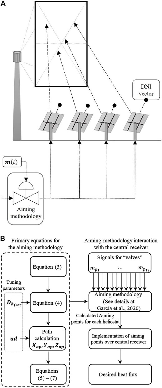
FIGURE 3. (A) Aiming methodology representation using the valve analogy. Adapted from (García et al., 2020) (B) Primary relations among equations within the aiming methodology calculation

2.3 Base Case

For $D_{h_{frac}}$, the base aiming methodology indicates that the tuning parameter moves between 0 and 1. The value for each heliostat was calculated as the ratio of two distances. The numerator is the distance between the heliostat and the tower. The denominator is the distance of the farthest heliostat in the solar field from the tower. The $ud$ parameter could be selected to move more aiming points toward the inlet of the fluid in the panel. This base case assumes that half of the aiming points go up and the other half down. Therefore, after applying the aiming methodology to the specific central receiver presented previously, the results (see Figure 4) confirmed the possibility of improving the performance of the last three panels. The lack of radiation in the middle of these last panels (recognizable by the pronounced u-shaped curve at Figure 4 for panels 7, 8, and 9) indicates that the $D_{h_{frac}}$ value was found too low for some of the aiming points. This implies that many of the aiming points left the equator of the panel and generated the flux profile seen in the panels. As explained in the aiming methodology, each section of aiming points was coordinated through the aperture percentage of the valve $\left(m\left(t\right)\right)$. These values were meant to come from a controller embedded in a closed loop. These values, enumerated in Table 2, were manually calculated for this base case until the heat flux was below the AFD by moving each one independently upward and downward.

FIGURE 4

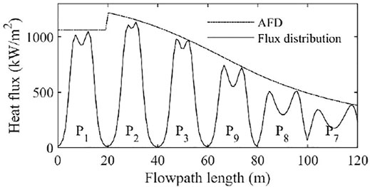
FIGURE 4. Heat flux distribution along flow path 1 using the aiming methodology with the default tuning parameters for $D_{h_{frac}}$ and $ud$.

TABLE 2

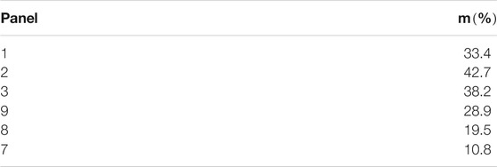
TABLE 2. Valve aperture percentages for the aiming points at each section for flow path 1.

2.4 Optimization Procedure

As stated in previous sections, the objective was to find suitable values for variables $D_{h_{frac}}$ and $ud$ for each heliostat in the solar field. Thus, instead of following an optimization procedure where each aiming point is given a value for those two variables, the proposed alternative included subdividing each section into smaller groups as follows:

• For variable $D_{h_{frac}}$, each section contained 10 subgroups (g_n), as shown in the shaded zone of Section 1 in Figure 5A. This avoided having too many variables to optimize, and in case some adjacent subgroups shared similar values, they were considered a larger subgroup.

• For variable $ud$, each section contained two subgroups (f_n). In one of them, the aiming points moved above the equator of the panel, and in the other one, the aiming points moved below this line (see the shaded area of Section 11 in Figure 5A).

FIGURE 5

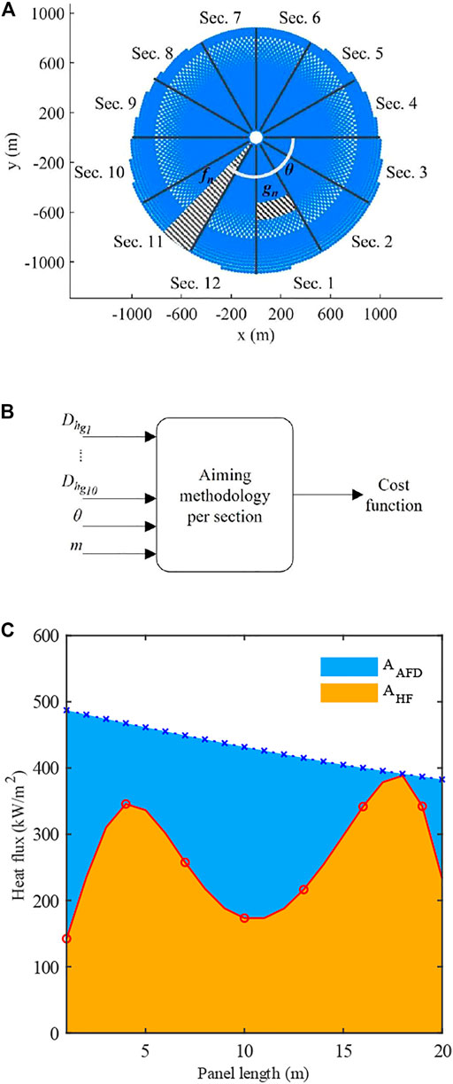
FIGURE 5. (A) Examples of subgroups g_n and f_n used for the optimization of variables $D_{h_{frac}}$ and $ud$ (B) General scheme of inputs and outputs for the optimization of one section of the solar field (C) Graphical representation of the areas used for the cost function.

For optimization, the angle $\theta$ between the coordinate that pointed to the west and the line that separated these two subgroups was modified. This angle was found to be positive for those sections located at the north of the solar field (Sections 4–9) and negative for the others. The final variable that was modified during optimization was the aperture percentage of the valve (m) for each section.

2.4.1 Cost Function

The output cost function, the ratio between the area below the flux distribution $\left(A_{HF}\right)$ and the area below the AFD $\left(A_{AFD}\right)$, was used to evaluate each set of values tested by the algorithm (see Figure 5C). The closer this value is to 1, the better the performance of the aiming strategy. Figure 5B shows the inputs and outputs for each section that the optimization procedure used to determine the most appropriate variables for $D_{h_{frac}}$ and $ud$.

2.4.2 Constraints

During optimization, three different kinds of constraints were taken into consideration. First, the obtained flux distribution was not allowed to go over the AFD at any point. Second, the value of $D_{h_{frac}}$ parameter was limited between 0.1 and 0.9, where the lower boundary avoided reaching 0, which could have caused some errors within the mathematical operations in the methodology. The upper bound avoided reaching a value of 1, which would imply that the aiming point is not moving. Third, the relative values of $D_{h_{frac}}$ were considered between subgroups. The possible configurations that were analyzed in this study are:

• Configuration 1: the $D_{h_{frac}}$ value of subgroup 1 (the closest subgroup to the tower) is lower than the value for subgroup 2, which is lower than the value for subgroup 3, and so on, i.e., $D_{h_{fra{c}_{g1}}}\le D_{h_{fra{c}_{g2}}}\dots \le D_{h_{fra{c}_{g10}}}$. This configuration ensures that the aiming points of heliostats closer to the receiver move farther from the equator of the panel toward the edges than those aiming points of heliostats far from the receiver.

• Configuration 2: this constraint makes the $D_{h_{frac}}$ value for subgroup 5 (in the middle of the section) have the largest value and the other lower ones. This configuration promotes that many aiming points stay near the equator to avoid the lack of energy seen in the base case.

• Configuration 3: this scenario withdraws the constraint and lets freely the optimization algorithm determine the $D_{h_{frac}}$ values for each subgroup.

2.4.3 Optimization Algorithm

The surrogate optimization algorithm, which is recommended when the objective function is time-consuming, was used in this study. It was realized using the Global Optimization Toolbox of MATLAB (MathWorks, 2021). This algorithm attempts a global optimum using fewer objective function evaluations by balancing exploration and speed.

3 Results and Discussion

This section discusses the effects of the optimal values on the system’s performance under on- and off-design scenarios.

3.1 Optimal Values

Regarding the optimal values for the tuning parameters, Table 3 shows that the constraints for configurations 1 and 2 were realized. That is, for configuration 1, vector $D_{h_{frac}}$ contained values close to 0.1 for those heliostats close to the receiver and 1 for those at the external edge of the section. For configuration 2, the optimization led to heliostats near the middle of the section staying close to the receiver’s equator. Thus, distant heliostats could move more than the middle ones, and closer heliostats to the receiver could move more to the edges of the panel. Moreover, Figure 6 displays an appreciation of the optimal values along the solar field. The distribution of aiming points up and down the panel was almost half for most sections. However, in panel 7, the aiming points tended to go more to the bottom of the panel because the fluid had a lower temperature, and therefore, the AFD was observed to be higher.

TABLE 3

TABLE 3. Results from the optimization procedure for each configuration.

FIGURE 6

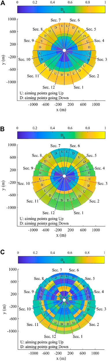
FIGURE 6. Values for $D_{h_{frac}}$ after optimization (A) Configuration 1 (B) Configuration 2 (C) Configuration 3.

3.2 On-Design Scenario Performance of the Optimal Values on the System

Figure 7 displays the flux profiles divided into several subplots to compare responses for all the previously established constraint configurations. It indicates that these behaved similarly to the base case, mainly for the first three panels. Nevertheless, regarding the last three panels, all the optimizations improved the response of the base case. In general, the performance of the base case was improved by 27%. For configuration 1, Figure 8A shows the 2-D heat flux distribution for the whole receiver; compared to the AFD in Figure 8B, the AFD was never exceeded for the whole receiver.

FIGURE 7

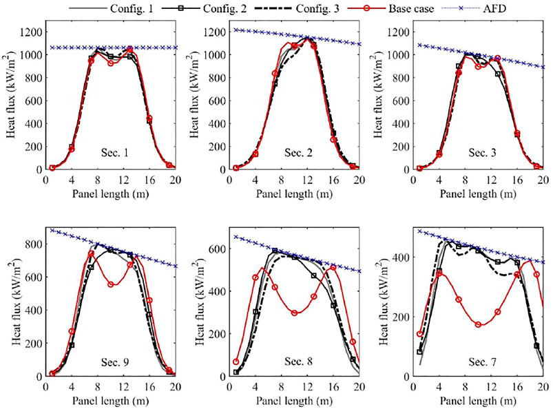
FIGURE 7. Heat flux distribution for each configuration and its comparison with the base case for flow path 1.

FIGURE 8

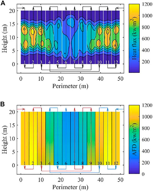
FIGURE 8. (A) 2-D heat flux distribution for configuration 1, and (B) the corresponding AFD at solar noon.

3.3 Off-Design Scenario Performance of the Optimal Values on the System

Another vital aspect analyzed in this study is the behavior of the aiming methodology under different scenarios. Using the same optimal values of $D_{h_{frac}}$ and θ for the mid-day case (configuration 1) in Table 3, the methodology was tested for the operating points explained in Figure 2C. It is important to remember that this aiming methodology was designed to work in a closed-loop strategy, and thus, values for the percentage of aperture (m) were required to be modified. These values were manually modified for different scenarios until the heat flux was at most equal to the AFD (See Table 4). It is also noteworthy that these were readily obtainable only after a few iterations. The results (see Figure 9A) showed that the flux distribution presents an appropriate distribution for all the panels, allowing most of the energy to reach the panel without surpassing the predefined AFD. For the 09:00 case, the flux required to reach the AFD in panels 1 and 3 was not reached, which means the energy delivered by the heliostats of that section was not enough at this time. For the 16:00 case, panel 2 showed a slight deviation to one side but did not inhibit the strategy to achieve an appropriate heat flux. In both scenarios, the last three panels of the flow path behaved as expected. The aiming points moved consistently to maintain, as much as possible, the shape of the flux profile seen in the solar noon case. It means that the collected energy is also close to the maximum collection value.

TABLE 4

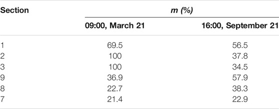
TABLE 4. Values for the valve aperture at each section for the two additional scenarios analyzed.

FIGURE 9

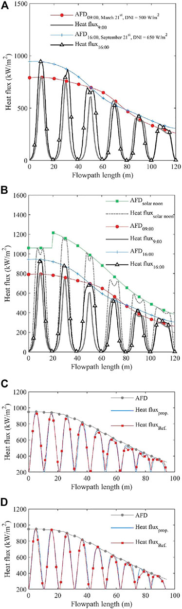
FIGURE 9. (A) Performance of the aiming strategy under different scenarios for DNI and time (B) Performance of the aiming strategy under different scenarios for DNI and time, using the same values for $D_{h_{frac}}$ in all sections as indicated in Table 5 (C) Comparison of the tuned aiming methodology to the results published by (Sánchez-González et al., 2016) (D) Comparison against the results given by (García et al., 2018).

As explained initially, the heat flux distribution of panel 7 was largely benefited from the optimized values calculated through the proposed methodology. Therefore, it is plausible to wonder if using the optimal values of $D_{h_{frac}}$ for panel 7 over all the panels in the receiver could give good flux profiles along the heating flow path. Besides keeping these values constant, the optimization procedure was executed to obtain the values for θ and m. Table 5 shows the parameters for the stated scenario, and Figure 9B shows the performance of the aiming methodology. Evidently, the aiming methodology could be tuned to cope with this new situation. All the panels presented an appropriate heat flux distribution either for the design scenario, at solar noon, or for the different days and times of operation. The results are remarkable as the values obtained through this study could be used to tune the aiming methodology in several configurations for the solar field and receiver.

TABLE 5

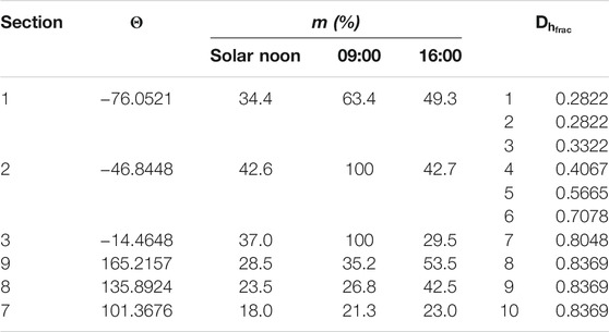
TABLE 5. Values for θ and m that allow using the same $D_{h_{frac}}$ values for all the sections.

3.3.1 Different Solar Field and Receiver Configuration

Previous results have indicated that the obtained values can be extrapolated to different scenarios. The final analysis conducted in this study involved using the same values for $D_{h_{frac}}$ presented in Table 5 over a different solar field and receiver. In this case, the configuration used the main features of the Gemasolar solar field in Spain (Sánchez-González et al., 2016). Table 6 shows the tuning parameters used in this case for the flow path on the west. The receiver contains 18 panels, nine per flow path, and the test considers half of the aiming points going up the equator of the receiver and the other half moving down. It implies that the values for θ are defined. Figure 9C and Figure 9D show the heat flux distribution using this scenario, compared against the results presented in the available literature. While it is not fair to compare against the results of optimal responses, this result shows the robustness of the tuning and how, by setting some parameters, the proposed aiming methodology can yield relevant results.

TABLE 6

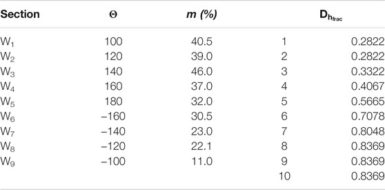
TABLE 6. Values for θ and m that allow using the same $D_{h_{frac}}$ values for all the sections of the Gemasolar solar field at solar noon during the summer solstice (DNI = 930 W/m²).

4 Conclusion

This paper elaborates on the tuning procedure and main details required to set an aiming methodology of heliostats toward a central receiver. The effect of two parameters, one that limits how far the aiming point of the heliostat can move from the equator line of the receiver, and another one that represents its direction (upward or downward) is described in detail in addition to an approach to modify them to attain the desired flux profile and accomplish the flux limits for a safe operation of the central receiver. The optimized values of the tuning parameters improved the base case scenario by 27% and showed how the same values produced appropriate flux distribution under off-design scenarios. The results also evidenced the robustness and flexibility of the aiming methodology through implementation into a different configuration of solar field and receiver. Finally, it was shown that the set of calculated values can be used as initial parameters for different configurations.

Data Availability Statement

The original contributions presented in the study are included in the article/supplementary material, further inquiries can be directed to the corresponding author.

Author Contributions

JG, RB, RV and DA contributed to the conception and design of this study. JG, RB and DA prepared the methodology. JG, RB and YC prepared the formal analysis. RB was in charge of finding the resources. DA, DE, and PV contributed to the interpretation of the results. JG, DA, and RB prepared the original draft. YC, RV and RB provided review and editing.

Funding

The authors would like to express their sincere gratitude to the Chilean Government, which funded this research through a postdoctoral project supported by the Comisión Nacional de Investigación Científica y Tecnológica (CONICYT), the Fondo Nacional de Desarrollo Científico y Tecnológico (FONDECYT), and Universidad Técnica Federico Santa María, postdoctoral grant number 3190542 (CONICYT FONDECYT/POSTDOCTORADO/3190542). The authors also express their sincere thanks for the financial support from the ANID/Fondap/15110019 “Solar Energy Research Center“-SERC-Chile.

Conflict of Interest

The authors declare that the research was conducted in the absence of any commercial or financial relationships that could be construed as a potential conflict of interest.

Publisher’s Note

All claims expressed in this article are solely those of the authors and do not necessarily represent those of their affiliated organizations, or those of the publisher, the editors and the reviewers. Any product that may be evaluated in this article, or claim that may be made by its manufacturer, is not guaranteed or endorsed by the publisher.

References

Acosta, D., Garcia, J., Sanjuan, M., Oberkirsch, L., and Schwarzbözl, P. (2021). Flux-feedback as a Fast Alternative to Control Groups of Aiming Points in Molten Salt Power Towers. Solar Energy 215, 12–25. doi:10.1016/j.solener.2020.12.028

CrossRef Full Text | Google Scholar

Ashley, T., Carrizosa, E., and Fernández-Cara, E. (2019). Continuous Optimisation Techniques for Optimal Aiming Strategies in Solar Power tower Plants. Solar Energy 190, 525–530. doi:10.1016/j.solener.2019.08.004

CrossRef Full Text | Google Scholar

Buck, R., and Schwarzbözl, P. (2018). “4.17 Solar Tower Systems,” in Comprehensive Energy Systems (Elsevier), 692–732. doi:10.1016/B978-0-12-809597-3.00428-4

CrossRef Full Text | Google Scholar

Crespi, F., Toscani, A., Zani, P., Sánchez, D., and Manzolini, G. (2018). Effect of Passing Clouds on the Dynamic Performance of a CSP tower Receiver with Molten Salt Heat Storage. Appl. Energ. 229, 224–235. doi:10.1016/j.apenergy.2018.07.094

CrossRef Full Text | Google Scholar

Flesch, R., Frantz, C., Maldonado Quinto, D., and Schwarzbözl, P. (2017). Towards an Optimal Aiming for Molten Salt Power Towers. Solar Energy 155, 1273–1281. doi:10.1016/j.solener.2017.07.067

CrossRef Full Text | Google Scholar

García, J., Chean Soo Too, Y., Vasquez Padilla, R., Beath, A., Kim, J.-S., and Sanjuan, M. E. (2018). Multivariable Closed Control Loop Methodology for Heliostat Aiming Manipulation in Solar Central Receiver Systems. J. Solar Energ. Eng. 140, 17. doi:10.1115/1.4039255

CrossRef Full Text | Google Scholar

García, J., Barraza, R., Soo Too, Y. C., Vásquez Padilla, R., Acosta, D., Estay, D., et al. (2020). Aiming Clusters of Heliostats over Solar Receivers for Distributing Heat Flux Using One Variable Per Group. Renew. Energ. 160, 584–596. doi:10.1016/j.renene.2020.06.096

CrossRef Full Text | Google Scholar

González-Gómez, P. A., Rodríguez-Sánchez, M. R., Laporte-Azcué, M., and Santana, D. (2021). Calculating Molten-Salt central-receiver Lifetime under Creep-Fatigue Damage. Solar Energy 213, 180–197. doi:10.1016/j.solener.2020.11.033

CrossRef Full Text | Google Scholar

Kiera, M. (1989). “Heliostat Field: Computer Codes, Requirements, Comparison of Methods,” in GAST—proceedings of the Final Presentation. Editors M. Becker, and M. Böhmer (Berlin: Springer), 95–113. doi:10.1007/978-3-642-83559-9_7

CrossRef Full Text | Google Scholar

Liao, Z., Li, X., Xu, C., Chang, C., and Wang, Z. (2014). Allowable Flux Density on a Solar central Receiver. Renew. Energ. 62, 747–753. doi:10.1016/j.renene.2013.08.044

CrossRef Full Text | Google Scholar

MathWorks, (2021). Global Optimization Toolbox User’s Guide R2021a. Available From: www.mathworks.com (Accessed September 14, 2021).

Google Scholar

Oberkirsch, L., Maldonado Quinto, D., Schwarzbözl, P., and Hoffschmidt, B. (2021). GPU-based Aim point Optimization for Solar tower Power Plants. Solar Energy 220, 1089–1098. doi:10.1016/j.solener.2020.11.053

CrossRef Full Text | Google Scholar

Papaelias, M., García Márquez, F. P., and Ramirez, I. S. (2018). “Concentrated Solar Power: Present and Future,” in Renewable Energies (Cham: Springer International Publishing), 51–61. doi:10.1007/978-3-319-45364-4_4

CrossRef Full Text | Google Scholar

Sánchez-González, A., Rodríguez-Sánchez, M. R., and Santana, D. (2017). Aiming Strategy Model Based on Allowable Flux Densities for Molten Salt central Receivers. Solar Energy 157, 1130–1144. doi:10.1016/j.solener.2015.12.055

CrossRef Full Text | Google Scholar

Sánchez-González, A., Rodríguez-Sánchez, M. R., and Santana, D. (2020). Allowable Solar Flux Densities for Molten-Salt Receivers: Input to the Aiming Strategy. Results Eng. 5, 100074. doi:10.1016/j.rineng.2019.100074

CrossRef Full Text | Google Scholar

Schwarzbözl, P., Pitz-Paal, R., and Schmitz, M. (2009). Visual HFLCAL - A Software Tool for Layout and Optimisation of Heliostat Fields. Proceedings. Available at: http://elib.dlr.de/60308/1/11354-Schwarzbozl.pdf (Accessed February 10, 2015).

Google Scholar

Soo Too, Y. C., García, J., Padilla, R. V., Kim, J.-S., and Sanjuan, M. (2019). A Transient Optical-thermal Model with Dynamic Matrix Controller for Solar central Receivers. Appl. Therm. Eng. 154, 686–698. doi:10.1016/j.applthermaleng.2019.03.086

CrossRef Full Text | Google Scholar

Speetzen, N., and Richter, P. (2021). Dynamic Aiming Strategy for central Receiver Systems. Renew. Energ. 180, 55–67. doi:10.1016/j.renene.2021.08.060

CrossRef Full Text | Google Scholar

Vant-Hull, L. L. (2002). The Role of "Allowable Flux Density" in the Design and Operation of Molten-Salt Solar Central Receivers. J. Solar Energ. Eng. 124, 165–169. doi:10.1115/1.1464124

CrossRef Full Text | Google Scholar

Wang, K., He, Y.-L., Xue, X.-D., and Du, B.-C. (2017). Multi-objective Optimization of the Aiming Strategy for the Solar Power tower with a Cavity Receiver by Using the Non-dominated Sorting Genetic Algorithm. Appl. Energ. 205, 399–416. doi:10.1016/j.apenergy.2017.07.096

CrossRef Full Text | Google Scholar

Wang, S., Asselineau, C.-A., Logie, W. R., Pye, J., and Coventry, J. (2021). MDBA: An Accurate and Efficient Method for Aiming Heliostats. Solar Energy 225, 694–707. doi:10.1016/j.solener.2021.07.059

CrossRef Full Text | Google Scholar