Study on the Production Decline Characteristics of Shale Oil: Case Study of Jimusar Field

The productivity of horizontal shale oil wells is low. To achieve cost-effective development, hydraulic fracturing techniques are often used. After hydraulic fracturing, wells have a high initial production rate. After a period of production, the production rate will decline rapidly and then remain low for an extended period of time. The study of the decline characteristics of horizontal wells is of great importance. We have collected development data from 94 horizontal wells in the Jimusar field. Some classical decline curve methods, such as the “power law–loss ratio” rate decline model, the stretch exponential equation, and the Duong decline curve, can be used to fit the production history. For example, Wells JHW018, JI172_H, and JI36_H were analyzed for production variations at different stages after the onset of production decline. On the basis of the performance of the parameters in typical wells, it was found that only Valko extended decline curves could be used to obtain satisfactory prediction results. A controlled fracture decline rate is proposed to describe the extent of the initial decline. The findings of this study can help for better predict of shale reservoir production after volume fracturing.

Introduction

With the rapid development of society and economy, the development rate of conventional natural gas can no longer meet the requirements of society for energy supply, and oil and gas developers are gradually shifting the focus of development to unconventional oil and gas resources. Shale oil and gas, as an important part of unconventional oil and gas resources, has huge development potential. According to the US Energy Information Administration, global recoverable reserves of shale gas are approximately equal to those of conventional natural gas, at 187 × 10¹² m³ and are widely distributed in Asia, Europe, North America, South America, and Africa.

Shale oil and gas is distinguished from conventional oil and gas by its very long extraction times and production cycles, in some cases 30–50 years or even longer, but the productivity of horizontal shale oil and gas wells is lower. To achieve cost-effective development, hydraulic fracturing techniques are often used. After hydraulic fracturing, the well has a very high initial production rate. After a period of production, the production rate will decline rapidly and then remain low for an extended period of time. Therefore, the study of the production decline characteristics of horizontal wells is of great importance to the development and production of oil and gas fields.

The prediction of shale reservoir decline is influenced by many factors such as geological complexity, the presence of natural fractures, ground stress state, completion and fracture characteristics, and multiphase flow characteristics (Kabir et al., 2011). The complex geological factors of fractures and the nadir permeability of the geological model make it difficult to use numerical simulation methods to predict producing wells. In addition, given the cost and time required for numerical simulations, operators typically use semi-analytical and empirical models. These methods require less data and allow for faster prediction results.

For reservoir evaluation based on the rate time data of gas wells produced under boundary dominant flow, Arps (1945) empirical hyperbolic decline model and related types of curves are usually used. For volumetric single-phase gas reservoirs produced under constant bottom hole pressure (BHP), the decline exponent b used in the Arps hyperbolic model can be calculated completely according to the fluid properties and bottom hole specifications at that time, without considering the reservoir properties and collecting any rate time data. Stumpf and Ayala (2016) applied the type curve and linear analysis technology obtained from the hyperbolic model. The reservoir properties of gas wells are successfully determined, and the prediction ability of the model is verified by numerical simulation and field data case study. Zhang and Ayala (2018) rederived the decline exponent for the change of variable BHP. The hyperbolic decline coefficient of variable BHP completely depends on the fluid PVT characteristics, and its amplitude is the largest compared with the production of constant-BHP.

At present, there are well-established methods for studying the declining production pattern (or dynamic analysis) of gas wells:the traditional Arps declining curve method, the classical Fetkovich typical curve fitting method, as well as the Blasingame typical curve fitting method and the Agarwal–Gradner typical curve fitting method (Yuan, 2016; Chen et al., 2018; Chong, 2019). For the study of the declining production pattern of shale gas wells, scholars in North America have proposed the exponential law declining method, the extended exponential declining method, etc (Sheng, 2016; Odi et al., 2019; Kocoglu et al., 2020; Wang and Ayala, 2020). In addition, some traditional methods can also be combined with the production characteristics of shale gas to improve the analysis and study of the declining production pattern and production history of shale gas (Ilk et al., 2008; Ilk et al., 2009).

The most commonly used decline curve analysis methods that have been historically applied to shale reservoirs are Arps (1945), Fetkovich (1980), Blasingame and Rushing (2005), Valko and Lee (2010), Duong (2010), Fulford and Blasingame (2013), and other methods. The Arps (1945), Fetkovich (1980), and Blasingame and Rushing (2005) methods were originally explored for conventional reservoir development and have certain limitations when applied to unconventional reservoir development. On the other hand, Valko and Lee (2010), Duong (2010), and Fulford and Blasingame (2013) methods are specifically developed for unconventional shale reservoirs. Here, we choose the classic Arps hyperbolic declining (AHD) curve method, the Valko stretched exponential decline (VSED) curve method, and the Duong harmonic declining (DHD) curve method to compare the decreasing predictions. Comparing the parameter fitting characteristics of typical wells, the most effective decline model is obtained by comparing the effectiveness of fitting parameters of three curves of 82 horizontal wells.

AHD Curve Method

Starting from the relationship between the rate of decline D and time, the rate of decline is approximated by the law of decay exponential function instead of the rate of decline in production, introducing a new equation for calculating the rate of decline D over time and distinguishing it from the hyperbolic decreasing rate of decline calculation.

Arps (1945) published three empirical formulas to predict the production performance of oil wells. They are exponential, hyperbolic, and harmonic. These equations are valid for reservoirs produced under constant BHP. It is assumed that the reservoir and fluid properties remain constant throughout the life of the well. In addition, the Arps empirical formula is valid only when the production well does not encounter any workover operations in the future. Table 1 shows three different Arps formulas. Arps hyperbolic and harmonic equations are more suitable for solution-gas-drive and water-drive reservoirs, whereas exponential equations are suitable for limited large reservoirs without pressure supply.

TABLE 1

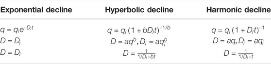
TABLE 1. Exponential, hyperbolic, and harmonic equations from Arps (1945).

In the Arps equations, q refers to the gas-production rate, q_i is the initial production rate, t refers to the time in days, D is the instantaneous decline rate, D_i is the initial decline rate, and b is the decline exponent.

VSED Curve Method

Valko (2009) proposed an extension exponential declining method to analyze the production history of tight formation gas or shale gas wells. The applicability of the method is proved by analyzing the production history of a large number of Barnett shale gas wells in the United States. Using the concept of extended exponential decay in mass in physics and applying it to the production decline of tight formation gas, it is stated that the production decline comes from the sum of many exponentially decayed single heterogeneous factors.

Table 2 shows the equation proposed by Valko and Lee (2010). Valko and Lee (2010) did not give the calculation equation for D in the original paper, and it can be calculated using the formula D = −1/q(dq/dt). Taking the logarithm on both sides, the parameters $\tau$ and n can be obtained by plotting log(D) (history fitting of production data) vs. log(t).

TABLE 2

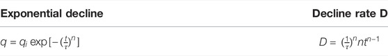
TABLE 2. Decline-curve equations proposed by Valko and Lee (2010).

DHD Curve Method

Duong (2010) proposed an empirical analysis method for gas well production decline for fractured shale gas reservoirs. On the basis of the analysis of the production history of a large number of Barnett shale gas wells in the United States, Duong stated that the production history of gas wells shows fractured linear flow over a long production period. This is mainly due to the relatively developed fractures in such shale gas reservoirs and the ultra-low permeability of the bedrock. In addition to fractures created by hydraulic fracturing, there are primary and later secondary fractures. It is difficult to produce gas wells with proposed radial flow and proposed steady-state flow controlled by selected boundaries.

Table 3 shows the equation proposed by Duong (2010). The equation of D is not given in the original paper but calculated using the formula D = −1/q(dq/dt). Duong stated that, for actual shale gas wells, the m value will always be greater than 1.0. If the m value is less than 1.0, then the gas well may be a conventional low-permeability formation gas well.

TABLE 3

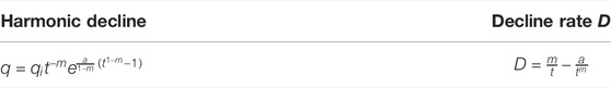
TABLE 3. Decline-curve equations proposed by Duong (2010).

Characteristics of Jimusar Shale Oil and Gas Development

Figure 1 shows the well location distribution of the Jimusar shale oil area. The Jimusar shale oil area was formally put into development in 2010. The shale oil has integrated source and reservoir, frequent interbeds, complex and changeable lithology, and no obvious source and reservoir. The characteristics of the boundary are obviously different from the North American Bakken marine shale oil and the Ordos continental shale oil. The Lucaogou Formation shale oil reservoir is a low-porosity and ultra-low permeability reservoir. The average porosity of the overburden porosity and permeability samples is 9.5%, and the permeability is 0.001 × 10⁻³ μm²∼0.6 × 10⁻³ μm²; Micropores dominate, and large-size nanopores and micropores are the main storage space for oil and gas. The “sweet spot” with porosity greater than 12% has an average oil saturation of 84%, and the “sweet spot” with a porosity of 8%–12% has an average oil saturation of 65%. On the plane, the properties of the crude oil from the Lucaogou Formation deteriorated from the middle of the depression to the edge, and the viscosity of the crude oil in the lower “sweet spot” was higher than that of the upper “sweet spot”. The average surface crude oil density of the upper “sweet body” is 0.88 g/cm³, the viscosity at 50°C is 50.27 mPas, and the formation crude oil viscosity is 10.58 mPas. The average surface crude oil density of the lower “sweet body” is 0.90 g/cm³, and the viscosity is 123.23 mPas at 50°C. Because of the poor physical properties of shale oil reservoirs and lack of continuous production capacity, it is difficult to achieve economic and effective production.

FIGURE 1

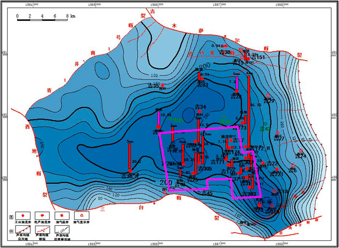
FIGURE 1. Jimusar shale oil field.

The development of the Jimusar shale oil area was implemented step by step (Zhang et al., 2011; Zhang et al., 2013). The first batch of horizontal wells were opened in 2012, 14 new wells were opened between 2012 and 2014, and two horizontal wells were developed and tested in 2016, and the output increased significantly. In 2018, 21 horizontal wells were deployed with the development method of “horizontal wells + subdivision-cut volume fracturing” to further determine the distribution of oil layers and explore reasonable horizontal well spacing (Zhou et al., 2014, Xi and Morgan, 2019). In 2018, the upper “sweet spot” put into operation nine horizontal wells with good production results. In 2019, a breakthrough was made in the production increase test of horizontal wells in the lower “sweet spot”. At the beginning of 2019, the planning and deployment plan for the whole district was completed. From 2012 to 2019, a total of 94 horizontal wells were completed and put into production, of which 14 wells were put into production for more than 3 years. The historical production characteristics of these 94 horizontal wells are summarized as follows:

(1) For wells that have been in production for more than 3 years, single well fluid production, oil production and oil pressure decline rapidly. After the decline trend is formed, it will soon enter the matrix control flow stage.

(2) The fluid production, water cut and flow pressure of most wells have stabilized within 3 years; wells that have been produced for less than 3 years are in the fracture-controlled production stage and have not yet entered the matrix-controlled production stage.

(3) Oil nozzle adjustment, pumping, fracturing, and workover have a significant impact on production and pressure (Weng and Siebrits, 2007; He and Gao, 2009; Wigwe et al., 2019a; Wigwe et al., 2019b; Wigwe et al., 2019c; Wigwe et al., 2020).

(4) Well production is affected by geological and engineering factors.

Take Well JHW018 as an example; the left part of the purple line in Figure 2 shows the production of Well JHW018 without fracturing, when the daily oil production was almost zero, whereas, to the right of the intersection of the nozzle size curve and the purple line, fracturing was carried out and gradually replaced by a larger size nozzle, the oil pressure drop rate gradually accelerated with the larger size of the nozzle, and the daily oil production increased rapidly while oil flow started to be produced, which indicates that the fracturing measures are effective. When the oil pressure drops rapidly as the nozzle size increases, the daily fluid production drops rapidly at the same time, and when the well is shut down for a period of time, the formation pressure recovers and the daily fluid production approaches the daily oil production when the well is opened again as the pressure stabilizes.

(5) The oil pressure declines quickly at the beginning of the well opening during the self-spout period, and the decline becomes slower in the later stage, and the smaller the oil pressure drop per unit fluid volume, the better the development effect.

(6) Some wells have pressure interference and inter-well connectivity.

(7) The morphology of the near-well fracture network caused by fracturing is obviously different.

FIGURE 2

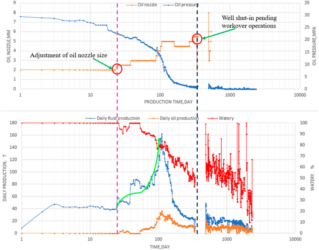
FIGURE 2. Production curve and nozzle oil pressure variation curve for Well JHW018.

The fracture network formed after fracturing Well JHW018 is of the perifracture SRV type, where there is generally no superposition of SRVs at each stage and cluster of fractures, so that, after fracturing, the fractures around the near-well first communicate with the bottom of the well, and daily fluid production gradually increases as more sheet fractures communicate with the bottom of the well. Production declines rapidly when all fractures communicate with the bottom of the well.

Research on Horizontal Well Production Decline Method

This chapter adopts the idea of using existing production dynamic data to perform regression and transformation to obtain a typical curve to establish a typical decline curve. The idea is as follows:

1) According to the differences in block wells’ planar physical properties, geochemical indicators, well types, productivity, production time, cumulative production, production system, production mode, etc. We select Jimusar representative wells with long production history.

The typical wells selected were all produced for more than 3 years, produced continuously or shut in for less than 10% of the production cycle, and produced continuously after reaching peak production. The values of the parameters (decreasing rate, decreasing index, etc.) obtained from the fitting of such production wells conform to the characteristics of a decreasing curve.

2) For fixed production wells, if the production decline has not yet occurred, on the basis of the principle of decline typical curve, then the difference of typical wells can be unified into the relationship between the two characterization indicators, and the indicators can be mathematically processed to establish a fitting Relations, extract the decreasing typical curve, and analyze its characterization significance.

3) For constant pressure production wells or blowout production wells, use a variety of classic decline theories to analyze and fit corresponding curves to predict future production and recoverable reserves and summarize the decline laws of these wells.

As shown in the Table 4, according to the differences in the plane physical properties, geochemical indicators, well types, productivity, production time, cumulative production, production system, and production methods of Jimusar shale reservoirs, 10 typical Jimusar reservoirs with representative and long production history are selected. Well, explore the typical curve of its production decline.

TABLE 4

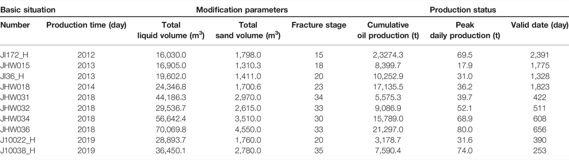
TABLE 4. Basic information of 10 typical wells in Jimusar.

Here, the processing method of Well JHW018, Well JI172_H, and Well JI36_H are used as the examples to briefly describe the analysis process of shale oil and gas reservoir production decline.

Find the peak value of daily oil production from Figure 3 and record it as q_i. As shown in Figure 4, record the peak value and subsequent production data, and use nonlinear fitting software to fit the three decreasing curves, respectively, and get the corresponding parameter value statistics are as follows.

FIGURE 3

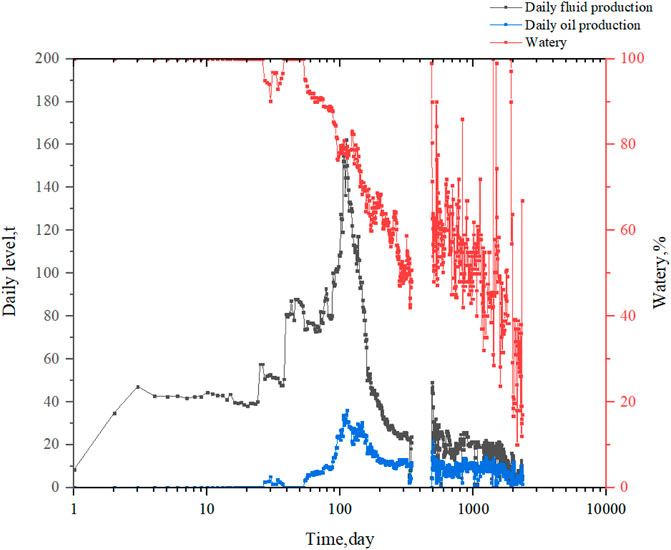
FIGURE 3. Production performance curve of Well JHW018.

FIGURE 4

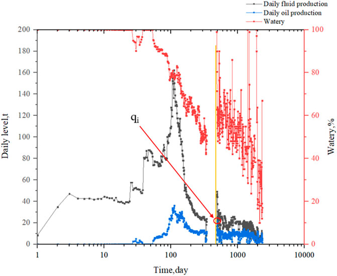
FIGURE 4. Production performance curve of Well JHW018.

Using the same processing method to obtain the q_i of Well JI172_H.

Figure 5; Figure 6 show the process of finding q_i for production data of Well JI172_H.

FIGURE 5

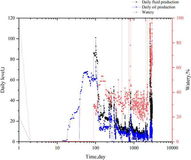
FIGURE 5. Production performance curve of Well JI172_H.

FIGURE 6

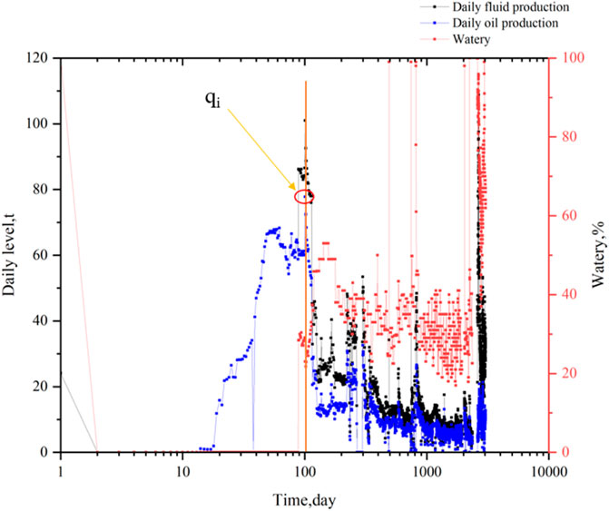
FIGURE 6. Production performance curve of Well JI172_H.

Using the same processing method to obtain the q_i of Well JI36_H.

Figures 7 and 8 show the process of finding q_i for production data of Well JI36_H.

FIGURE 7

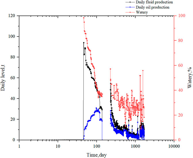
FIGURE 7. Production performance curve of Well JI36_H.

FIGURE 8

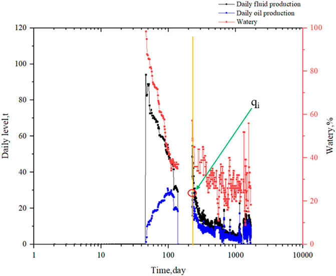
FIGURE 8. Production performance curve of Well JI36_H.

It can be easily said that the most time-consuming part of this part of the work is to use the history fitting method to obtain the parameter values of the three types of curves. As shown in Table 5, we will sort out the results obtained and sort out the parameter data of typical wells for analysis (Pan et al., 2014).

TABLE 5

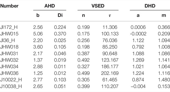
TABLE 5. Fitting parameters of 10 typical horizontal wells.

The peak of both Well JHW018 (Figure 4) and Well JI36_H (Figure 8) occurred after volumetric fracturing, and these two groups formed a control group to compare the change in production after fracturing. As mentioned earlier, Well JHW018 produced much more fluid per day than oil per day before fracturing and produced steadily for over 1,000 days after forming a SRV-developed fracture network around the fracture. Well JI36_H had a peak after shut-in fracturing close to the pre–shut-in peak production, with production declining rapidly after the end of fracture flow due to intra-volume fracturing to communicate the fractures and low permeability of the unfractured matrix. For Well JI_172H (Figure 6), which was the first well to be volumetrically fractured as an experimental well at the beginning of production and produced continuously and steadily, the best historical fit was achieved for Well JI_172H when comparing Well JHW018 and JI36_H.

By observing Figure 3 to Figure 8, it can be seen that the three wells were shut down for a period of time before the peak production appeared. After the well was opened again, the water cut fluctuated drastically, and the beginning of the production decline basically coincided with the severe water cut fluctuating time. For the rapid decline in production, it is speculated that this is related to the continuous expansion of the area affected by water flooding. Combined with the microseismic detection result map of Well JHW018, the effect of horizontal well + volume fracturing is limited, and production can only be increased in a short time. For long-term stable and high production, it is still necessary to improve technology or develop new technologies.

The point matrix in Figure 9 is a horizontal projection of the microseismic test performed after volumetric fracturing of Well JHW018, characterizing the fracture scale and fracture pattern, corresponding to the production characteristics of Well JHW018. The size of the modification volume has a large impact on the late production of multi-stage fractured horizontal wells, mainly because the large modification volume reduces the fluid flow resistance after the late pressure wave propagates beyond the modification area, and the production rises rapidly at the beginning of the modification, reaches a peak and then declines rapidly and remains at a certain lower production rate. The rise in yield occurs during the retrofit volume with low flow resistance and fast flow velocity, the pressure wave propagates outside the retrofit volume and the yield decreases to a certain lower constant value, when seepage within the matrix occurs with high flow resistance and low flow velocity.

FIGURE 9

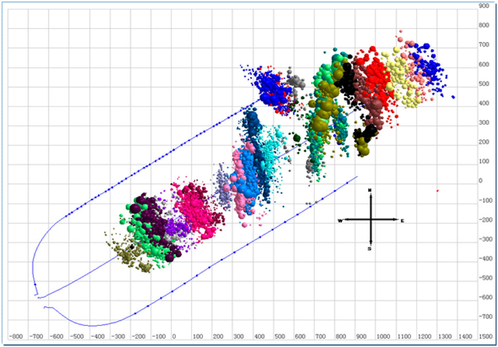
FIGURE 9. Well JHW018 microseismic detection result map (local SRV type).

According Figure 9 showing Well JHW018(local SRV type) microseismic detection result map, it was transformed into a high production well after volume fracturing.

Observing the fitting results in Figure 10, it can be seen that, for Well JHW018, the simulation effects of the three curves are very similar. Only in the early stage of production decline, there are obvious differences in the fitting results. It is speculated that this fitting result is due to the sufficient production data of this production well. The difference between the three declining fitting curves is very small, which also confirms the applicability of the three declining curves.

FIGURE 10

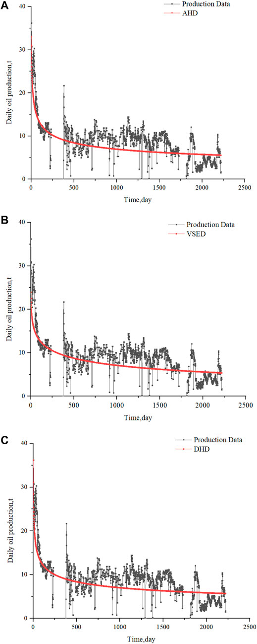
FIGURE 10. Three decreasing fitting curves of Well JHW018: (A) AHD fitting curve of Well JHW018, (B) VSED fitting curve of Well JHW018, and (C) DHD fitting curve of Well JHW018.

Observing the fitting results in Figure 11, it can be seen that, for Well JI172_H, the three curve fitting results are very close, and the fitting is close to the actual production data during the rapid decline stage of production. The Well JI172_H was shut down from 2,250 to 2,500 days after the beginning of the production decline. After the well was opened again, the production recovered somewhat. The curve fitting results have a large deviation from the production data. This is not a problem of the fitting curve itself but more affected by engineering geological factors.

FIGURE 11

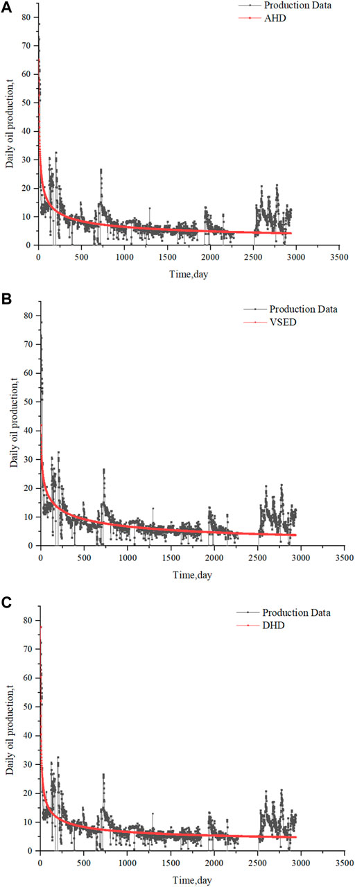
FIGURE 11. Three decreasing fitting curves of Well JI172_H: (A) AHD fitting curve of Well JI172_H, (B) VSED fitting curve of Well JI172_H, and (C) DHD fitting curve of Well JI172_H.

Observing the fitting results in Figure 12, it can be seen that, for Well JI36_H, VSED curve of the three curves is the closest to the production history, and AHD and DHD only have a better fitting effect within the first 50 days of the production decline. Similar to Well JI172_H, Well JI36_H also adjusted the production situation through shutdown adjustments. When the well was opened again, it was affected by engineering geological factors, and the decline curve could no longer fit the actual production well.

FIGURE 12

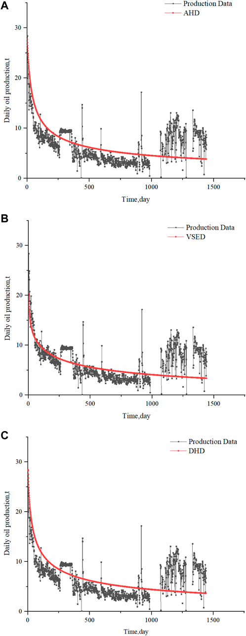
FIGURE 12. Three decreasing fitting curves of Well JI36_H: (A) AHD fitting curve of Well JI36_H, (B) VSED fitting curve of Well JI36_H, and (C) DHD fitting curve of Well JI36_H.

Conclusion

Shale reservoirs are matrix and fracture dual pore media, but the adsorption and diffusion characteristics of shale reservoirs make shale gas reservoirs different from conventional oil and gas reservoirs. In this paper, the declining production pattern of 82 horizontal wells in the Jimusar shale reservoir is analyzed by the declining curve analysis method proposed by domestic and foreign scholars, and the declining influencing factors are analyzed. The conclusions are as follows:

① Three typical wells with long production histories were selected: Well JI172_H, Well JI36_H, and Well JHW018. JI36_H was the best fit because it produced continuously after reaching peak production and was shut in for a short period of time before production was suspended. Similarly, Well JHW018, which was shut-in 200–400 days after peak, did not fit as well as Well JI36_H.

② The number of valid wells for the three curve fits totaled 55 (red font in Supplementary Appendix A), excluding wells with low data volumes, no production peaks, and wells with multiple workovers or shut-ins. For the AHD curve, the number of validly fitted wells is 31 (b>1,0 < D_i < 1), removing three of them that do not meet the fitting parameters, i.e., b < 0 (marked in green in Supplementary Appendix A); for the VSED curve, the number of validly fitted wells is 36 (0 < n < 1, 50<τ < 200), removing 4 of them, i.e., n < 0 (marked in green in Supplementary Appendix A); for the DHD curve, the number of validly fitted wells is 14 (a≈1, m > 1), removing 19 of them, i.e., a<0 (marked in green in Supplementary Appendix A). According to statistics obtained, the DHD method has the lowest success rate of effectively fitting production, so it is no longer suitable for forecasting shale oil and gas production. Both the VSED curve and the AHD curve can fit production history of most horizontal wells, and the VSED can obtain more satisfactory prediction results.

③ In response to the characteristics of fast decreasing production of Jimusar shale oil, wells that have been in production for more than 2 years can be considered to be in the middle to late stage of self-injection production, when the activated reserves mainly originate from the matrix, and the preliminary modification process has less influence on production and geological factors have more influence. To increase production, it is recommended to adopt the technology of horizontal well + volume fracturing and constant flow production, so as to prevent the rapid decline of initial production.

Data Availability Statement

The original contributions presented in the study are included in the article/Supplementary Material, further inquiries can be directed to the corresponding author.

Author Contributions

SL is the main author of the thesis, supervised by HS.

Conflict of Interest

Author SL was employed by the Xinjiang Oilfield Company, PetroChina. The remaining author declares that the research was conducted in the absence of any commercial or financial relationships that could be construed as a potential conflict of interest.

Publisher’s Note

All claims expressed in this article are solely those of the authors and do not necessarily represent those of their affiliated organizations or those of the publisher, the editors, and the reviewers. Any product that may be evaluated in this article, or claim that may be made by its manufacturer, is not guaranteed or endorsed by the publisher.

Supplementary Material

The Supplementary Material for this article can be found online at https://www.frontiersin.org/articles/10.3389/fenrg.2022.845651/full#supplementary-material

References

Arps, J. J. (1945). Analysis of Decline Curves. Trans. AIME 160 (01), 228–247. doi:10.2118/945228-g

CrossRef Full Text | Google Scholar

Blasingame, T. A., and Rushing, J. A. (2010). “A Production-Based Method for Direct Estimation of Gas in Place and Reserves,” in Paper presented at the SPE Eastern Regional Meeting, Morgantown, WV, September 2005. doi:10.2118/98042-MS

CrossRef Full Text | Google Scholar

Chen, X., Zhang, G., Kang, Y., and Xu, D. (2018). Numerical Simulation of Shale Reservoir Volume Fracturing Considering Natural Fractures[J]. Chin. Sci. Technol. Paper 13 (03), 286–290.

Google Scholar

Chong, Z. (2019). Analysis of Production Decline Factors of Fracturing Horizontal wells in Tight Reservoirs and Study of Decline Law. IOP Conf. Ser. Mater. Sci. Eng. 563 (3), 032005. doi:10.1088/1757-899x/563/3/032005

CrossRef Full Text | Google Scholar

Duong, A. N. (2010). “An Unconventional Rate Decline Approach for Tight and Fracture-Dominated Gas Wells[C],” in Canadian unconventional resources and international petroleum conference. Society of Petroleum Engineers.

Google Scholar

Fetkovich, M. J. (1980). Decline Curve Analysis Using Type Curves[J]. J. Petrol. Technol. 32 (06), 1065–1077.

CrossRef Full Text | Google Scholar

Fulford, D. S., and Blasingame, T. A. (2013). “Evaluation of Time-Rate Performance of Shale Wells using the Transient Hyperbolic Relation,” in Paper presented at the SPE Unconventional Resources Conference Canada, Calgary, Alberta, Canada, November 2013. doi:10.2118/167242-MS

CrossRef Full Text | Google Scholar

He, J., and Gao, H. (2009). Pressure Dynamic Analysis of Dual-Medium Reservoirs with Multiple Fracturing Fractures[J]. J. Oil Gas Technol. 31 (03), 130–133+8.

Google Scholar

Ilk, D., Rushing, J. A., and Blasingame, T. A. (2009). “Decline-curve Analysis for HP/HT Gas wells: Theory and Applications[C],” in SPE Annual Technical Conference and Exhibition. Society of Petroleum Engineers.

Google Scholar

Ilk, D., Rushing, J. A., Perego, A. D., and Blasingame, T. A. (2008). “Exponential vs. Hyperbolic Decline in Tight Gas Sands: Understanding the Origin and Implications for reserve Estimates Using Arps' Decline Curves[C],” in SPE annual technical conference and exhibition. Society of Petroleum Engineers.

Google Scholar

Kabir, S., Rasdi, F., and Igboalisi, B. (2011). Analyzing Production Data From Tight Oil Wells[J]. J. Canad. Petrol. Technol. 50 (05), 48–58.

CrossRef Full Text | Google Scholar

Kocoglu, Y., Wigwe, M. E., Sheldon, G., and Watson, C. (2020). “Machine Learning Based Decline Curve—Spatial Method to Estimate Production Potential of Proposed Wells in Unconventional Shale Gas Reservoirs[C],” in Unconventional Resources Technology Conference, 20–22 July 2020. Unconventional Resources Technology Conference (URTeC), 499–517.

Google Scholar

Odi, U., Bacho, S., and Daal, J. (2019). “Decline Curve Analysis in Unconventional Reservoirs Using a Variable Power Law Model: A Barnett Shale Example[C],” in Unconventional Resources Technology Conference, Denver, Colorado, 22-24 July 2019. Unconventional Resources Technology Conference (URTeC); Society of Exploration Geophysicists, 4925–4949.

Google Scholar

Pan, L., Zhang, S., Cheng, L., Lu, Z., and Liu, K. (2014). Numerical Simulation of Inter-cluster Interference in Multi-Stage and Clustered Horizontal Well Fracturing[J]. Nat. Gas Industry 34 (01), 74–79.

Google Scholar

Sheng, C. (2016). Optimization of Cluster Perforation Parameters for Shale Gas Horizontal wells Based on Formation characteristics[D]. Beijing: China University of Petroleum.

Google Scholar

Stumpf, T. N., and Ayala, L. F. (2016). Rigorous and Explicit Determination of Reserves and Hyperbolic Exponents in Gas-Well Decline Analysis. SPE J. 21, 1843–1857. doi:10.2118/180909-pa

CrossRef Full Text | Google Scholar

Valkó, P. P. (2009). “Assigning Value to Stimulation in the Barnett Shale: A Simultaneous Analysis of 7000 Plus Production Hystories and Well Completion Records,” in Paper presented at the SPE Hydraulic Fracturing Technology Conference, The Woodlands, TX, January, 2009. doi:10.2118/119369-MS

CrossRef Full Text | Google Scholar

Valkó, P. P., and Lee, W. J. (2010). “A Better Way to Forecast Production from Unconventional Gas Wells[C],” in SPE Annual technical conference and exhibition. Society of Petroleum Engineers.

Google Scholar

Wang, Y., and Ayala, L. F. (2020). Explicit Determination of Reserves for Variable-Bottomhole-Pressure Conditions in Gas Rate-Transient Analysis. SPE J. 25, 369–390. doi:10.2118/195691-pa

CrossRef Full Text | Google Scholar

Weng, X., and Siebrits, E. (2007). “Effect of Production-Induced Stress Field on Refracture Propagation and Pressure Response[C],” in SPE Hydraulic Fracturing Technology Conference. Society of Petroleum Engineers.

Google Scholar

Wigwe, M. E., Bougre, E. S., Watson, M. C., and Giussani, A. (2020). “Spatio-temporal Models for Big Data and Applications on Unconventional Production Evaluation[C],” in Unconventional Resources Technology Conference, 20–22 July 2020. Unconventional Resources Technology Conference (URTeC), 3211–3230.

Google Scholar

Wigwe, M. E., Watson, M. C., Giussani, A., Nasir, E., and Dambani, S. (2019a). “Application of Geographically Weighted Regression to Model the Effect of Completion Parameters on Oil Production & Ndash; Case Study on Unconventional Wells[C],” in SPE Nigeria Annual International Conference and Exhibition.

Google Scholar

Wigwe, M. E., Westfall, P. H., Watson, M., Giussani, A., and Nasir, E. (2019b). Evaluation of the Effect of Well Parameters on Oil Production[J]. JSM Proc. Stat. Comput. Section, 1781–1803.

Google Scholar

Wigwe, M., Kolawole, O., Watson, M., Ispas, I., and Li, W. (2019c). “Influence of Fracture Treatment Parameters on Hydraulic Fracturing Optimization in Unconventional Formations[C],” in ARMA-CUPB Geothermal International Conference. American Rock Mechanics Association.

Google Scholar

Xi, Z., and Morgan, E. (2019). Combining Decline-Curve Analysis and Geostatistics to Forecast Gas Production in the Marcellus Shale. SPE Reservoir Eval. Eng. 22 (04), 1562–1574. doi:10.2118/197055-pa

CrossRef Full Text | Google Scholar

Yuan, F. (2016). Research on the Law of Single Well Production Decline in JY Shale Gas Reservoir. Chengdu, China: Southwest Petroleum University.

Google Scholar

Zhang, J., Li, J., Shi, X., Jiang, H., Huang, X., and Cai, X. (2013). Exploration and Practice of Tight Oil Fracturing Technology in Jimusar Depression[J]. Xinjiang Pet. Geology. 34 (06), 710–712.

Google Scholar

Zhang, J., Teng, X., Qiu, L., and Zhu, W. (2011). Case Analysis and Technical Countermeasures of Inter-well Interference during Infill Well Fracturing[J]. Pet. Geology. Eng. 25 (01), 95–97+145.

Google Scholar

Zhang, M., and Ayala, L. F. (2018). A Semi-Analytical Solution to Compositional Flow in Liquid-Rich Gas Plays. Fuel 212, 274–292. doi:10.1016/j.fuel.2017.08.097

CrossRef Full Text | Google Scholar

Zhou, Q., Robert, D., Kleit, A., and Wang, J. Y. (2014). Evaluating Gas Production Performances in marcellus Using Data Mining Technologies[C]. J. Nat. Gas Sci. Eng. 20, 20–36. doi:10.1016/j.jngse.2014.06.014

CrossRef Full Text | Google Scholar