 Andrzej Czyżewski
- Multimedia Systems Department, Faculty of Electronics, Telecommunications and Informatics, Gdańsk University of Technology, Gdańsk, Poland
Implementation of remote monitoring technology for real wind turbine structures designed to detect potential sources of failure is described. An innovative multi-axis contactless acoustic sensor measuring acoustic intensity as well as previously known accelerometers were used for this purpose. Signal processing methods were proposed, including feature extraction and data analysis. Two strategies were examined: Mel Frequency Cepstral Coefficients pruned with principal component analysis and autoencoder-based feature extraction. The scientific experiment resulted in data gathering and analysis to predict potential wind turbine mechanism failures.
1 Introduction
Wind turbines require constant monitoring for damage and irregularities. Such factors as deposits on rotor blades (requiring periodic cleaning), damage resulting from wear and tear of materials (e.g., bearings, oil), mechanical damage (e.g., the impact of heavy objects), and construction and material defects are taken into account. The primary method of damage detection is a periodic inspection by technicians. However, it is not a sufficiently effective solution as it does not allow for the quick detection of irregularities. Furthermore, damage to a turbine results in a decrease in generated power output and an increase in generated noise. Consequently, it may lead to rising energy production costs, damage the entire turbine, or even its permanent destruction. Therefore, automated systems are being developed that continuously monitor the condition of wind turbines to reduce the cost of their maintenance and help detect any deviations from the norm as quickly as possible.
Monitoring of noise from wind farms is primarily used to determine the degree of annoyance of wind turbines to nearby residents. Although wind turbines are considered to be an environmentally friendly source of energy, there is a lot of controversy about their presence near buildings. The main problem is the noise generated by turbines, which has a specific, amplitude-modulated character. Many studies try to prove the negative influence of noise on inhabitants, pointing to effects such as sleep disorders, bad mood, migraines, neurosis, etc. On the other hand, proponents of wind farms try to refute these theories with relevant research. In both cases, the primary tool is monitoring the level and nature of noise from wind turbines (Deshmukh et al., 2019). An example of such a study is the paper (Castellani et al., 2020), in which tower vibrations are measured and analyzed. In addition, a test case of a faulty wind turbine bearing (information provided by the manufacturer) is studied. An interesting intuition of that study is that the statistical novelty of the faulty signal can be enhanced by measuring vibrations at more than one wind turbine simultaneously and by analyzing the difference between the target wind turbine and references.
Noise generated by wind turbines can also have useful applications. Long-term noise analysis and detection of deviations from regular character can be helpful in detecting damage to a wind turbine, especially rotor blades. This topic is not sufficiently studied and described in the literature. Most wind turbine condition monitoring systems use “contact” sensors (accelerometers and microphones) placed directly on the turbine components. Meanwhile, as the author and his co-workers showed, contactless acoustic and video monitoring have the potential for investigating wind turbine conditions (Cygert and Czyzewski, 2018; Czyżewski, 2019).
The research project was carried out, employing the methods and results shown in this article, including using different sensors that record and analyze the sound generated by wind turbines, especially the acoustic intensity sensor that measures the acoustic speed and pressure.
The following assumptions were formulated in the research work, which should be fulfilled by the developed vibroacoustic and acoustic analyzer of the wind turbine condition. The first scenario assumes the monitoring of the wind turbine utilizing measurement sensors located at a certain distance from the wind turbine. Hence, in this first measurement scenario, labeled SC1 (External Analyzer), the following parameters can be monitored:
⁃ environmental noise emitted by the turbine, in particular blade noise, the expected result is an assessment of the blade sheath condition, the realization of the functionality will be achieved by using environmental microphones and/or a 3D intensity probe,
⁃ vibrations of the turbine tower, the functionality will be realized by using a special sensor called inclinometer,
⁃ an inspection of the wind turbine condition performed from an unmanned aerial vehicle (drone), in this case, a drone with a vision camera can be used, mounted in a specialized mount to eliminate vibrations of the aircraft, the acquired vision material containing images of selected elements of the turbine, in particular the blade surface, may be analyzed using proprietary digital image processing algorithms to support the detection of sheathing damages.
The second scenario assumes that the wind turbine is monitored using measurement sensors located inside the wind turbine nacelle. This measurement scenario has been designated as SC2 (Internal Analyzer). The following parameters can be monitored:
⁃ distribution of sound intensity inside the nacelle, with the possibility to indicate the source of noise, the functionality will be realized by using a 3D vector intensity probe, enabling detection of the arrival of the front of the acoustic wave,
⁃ vibrations inside the nacelle monitored by accelerometers.
For the research, the concept of a method for processing signals from sensors monitoring a wind turbine was developed.
Both scenarios were put into practice, yielding research results. The research description associated with the first scenario is treated in this article abbreviated but shows the use case of the constructed acoustic intensity probe working outside the turbine. The second scenario is related to the diagnostics of turbine mechanisms conducted in the interior of the turbine nacelle. In this case, the paper shows in a detailed way how acoustic signals are processed to observe the turbine mechanism working. The feature extraction methods and an application of the machine learning method (autoencoder) are discussed and presented with hitherto obtained results.
An overview of the issues involved is presented before the measurement methods, the equipment used for this purpose, and the means of data analysis related to the research project are shown.
2 Noise Sources in Wind Turbines
Noise generated during the operation of a wind turbine can be divided into two types: mechanical noise, associated with the elements inside the nacelle, and aerodynamic noise, related to the rotation of the blades and the influence of the wind (Deshmukh et al., 2019). Mechanical noise can be transmitted through the air (air-borne) and turbine structures (structure-borne). The primary sources of mechanical noise are (Rogers et al., 2002):
⁃ transmission,
⁃ generator,
⁃ the nacelle swivel system,
⁃ fans,
⁃ auxiliary equipment, e.g., hydraulic.
Due to the high height of the nacelle above the ground, the confinement of equipment inside the nacelle, and the use of sound attenuation systems, mechanical noise is generally not a nuisance to residents (unlike aerodynamic noise) but can be necessary for acoustic monitoring of turbine condition.
Aerodynamic noise is associated with wind movement and the phenomena that occur when an airstream falls on a wind turbine. The three most important factors causing aerodynamic noise are listed below (Oerlemans, 2011a; Okada et al., 2015).
⁃ Low-frequency sounds and infrasound are produced if the rotor blades cross local airflow minima caused by wind flow around the tower, changes in wind strength, etc.,
⁃ The turbulence created when the air stream falls on the front edge of the rotor blade makes noise.
⁃ The cutting of the air stream through the blade tip causes a vortex (tip vortex), resulting in acoustic waves,
⁃ The most important source of aerodynamic noise is air turbulence generated at the blade trailing edge (trailing edge flow). It results in a band noise (typically from 770 Hz to 2 kHz), although tonal components may also appear if blade damage is present. Importantly, for a stationary observer on the ground, this noise is amplitude-modulated by the rotor blade rotation (an effect referred to in English as swish), increasing its annoyance to listeners.
The airstream impinging on the rotor blade adheres, forming a turbulent boundary layer. As a result, the air moves along the blade cross-section (airfoil), hitting a sharp back edge where the air turbulence detaches from the blade surface, causing sound waves. This is the leading cause of aerodynamic noise in wind turbines (Oerlemans, 2011a). Okada made a detailed measurement of the directional characteristics of wind turbine noise (Okada et al., 2015). The noise level distribution in the horizontal plane for different frequencies and different turbine speeds reveals that the characteristics are octahedral in shape; a higher noise level was recorded on the wind axis and a lower noise level of about 5 dB on the lateral direction. The noise level decreases as the measured frequency band increases. Increasing the rotational speed obviously increases the noise level.
Amplitude modulation of wind turbine noise is the subject of much ongoing research (RenewableUK, 2013). Ordinary amplitude modulation, as described earlier, causes noise level fluctuations of up to 6 dB. It is audible only in the vicinity of the turbine (at a distance of up to about two rotor diameters); at greater distances, it disappears. However, the modulation effect is observed at much greater distances (in residential buildings), the amplitude of modulation is much greater, and it varies in time. This effect is called enhanced amplitude modulation (EAM). The causes of EAM in wind turbines have not yet been sufficiently explained. Factors such as changes in wind strength and direction, interactions of noise from different turbines in the farm, interactions between rotor and tower, inaccuracies in nacelle positioning relative to wind directions, and others have been reported (Bowdler, 2008; Oerlemans, 2011b).
Moller studied low-frequency sounds and infrasound propagation around wind turbines (Mollasalehi et al., 2017). The results indicate that the larger the turbine rotor diameter and higher the turbine power, the more energy is concentrated, and the lower the frequency range. Low-frequency noise is disruptive to the environment due to less attenuation of sound waves in this range (more extensive noise range). Turbines emit infrasound, but their level is lower than the threshold of human perception in this range.
3 Condition Monitoring of Wind Turbines
Wind farms require constant monitoring to detect at early stage irregularities that may cause permanent damage to the wind turbine and increase the level of generated noise. The primary monitoring method is an inspection performed by operators. However, it is cumbersome, time-consuming, and costly; therefore, it is performed only periodically, which may cause significant irregularities to be overlooked. Furthermore, a technician cannot notice every defect since hidden defects can be challenging to detect. Human monitoring can be preventive (inspection to find abnormalities that may lead to damage to turbine components) and corrective (repair of damaged components) (García Márquez et al., 2012). Preventive monitoring involves replacing worn parts (oil, filters) and tightening fastening bolts.
Since ad hoc inspection monitoring is not sufficient to ensure the continuous operation of wind farms, automated systems for constant monitoring of wind turbines play a vital role. The issue of condition monitoring is referred to as condition monitoring (CM). Systems oriented towards the detection of abnormalities in the operation of wind turbines are called Condition Monitoring Systems (CMS), while systems that monitor damage to the turbine structure (e.g., cracks) are called Structural Health Monitoring (SHM) (Coronado and Fischer, 2015; Fuentes et al., 2020).
CMS systems consist of a set of sensors placed on wind turbine components and a data analysis system, in practice, a computer with software implementing advanced data analysis algorithms. The general principle of CMS systems can be stated as follows: “any significant change in the measured parameters is an indicator of system malfunction.” (Pedregal et al., 2009). Monitoring can be carried out online (analysis on the fly and on-site) or offline (analysis of data collected for a certain period of time, carried out in the monitoring center). The most important turbine components to be observed are rotor blades, gearbox, generator, main bearing, and tower structure.
Modern condition monitoring systems for wind turbines are primarily based on monitoring vibrations of rotating elements of the power transmission system, namely, the main bearing, gearbox (bearings, shafts, gears), generator bearing, and frequent vibrations of the tower itself. Systems of this type have become well established in the wind turbine market and have proved useful in practice in many cases. For this reason, they are recommended as standard equipment for multi-megawatt wind turbines and offshore wind farms (Gellermann, 2013). Most of the sensors used in condition monitoring systems based on vibration analysis are accelerometers installed at specific locations in the power train. Different types of accelerometers are used in wind turbines, measuring from very low to high frequencies. The selection of a sensor requires consideration of the frequency range and the dynamic range and sensitivity of the sensor. It is important, for example, at low frequencies where the acceleration amplitudes may be very small, less than 1 mg. Selection of the sensor type can be carried out based on ISO 13373-1 (International standard ISO 13373-1, 2002), which provides an overview of commonly used transducer types, together with frequency ranges suitable for particular applications. Standard terminology for the various sensors used in wind turbine condition monitoring systems and their recommended positioning and orientation are listed in ISO 61400-25-6 (International standard ISO 61400-25-6, 2010). In addition, general requirements and recommendations for sensor positioning are given in the 2013 certification guidelines of the Germanischer Lloyd (DNV-GL) classification society. (Germanischer Lloyd, 2018). For example, one sensor should be used for the rotor bearing and four for the gearbox, in the range of 0.1 Hz–10 kHz.
3.1 Modalities and Analysis Methods for Wind Farm Monitoring
Modern CMS systems used in wind farms use many techniques and modalities. The most important ones are (Pedregal et al., 2009):
⁃ vibration analysis with accelerometers, most commonly used for gears and bearings,
⁃ acoustic emission testing using miniature microphones applied to both mechanical systems (mainly bearings) and aerodynamic components (rotor blades),
⁃ ultrasonic testing, used primarily for tower and rotor blade damage monitoring,
⁃ analysis of oil condition in mechanical systems (mainly in the gearbox),
⁃ stress (strain) analysis, applied principally to rotor blades,
⁃ electrical signal analysis - used to monitor the generator
⁃ shock pulse method (SPM) - used in bearing monitoring,
⁃ radiographic analysis, i.e., X-ray imaging of turbine elements - for obvious reasons, it is used only temporarily and is expensive, although it is also effective in detecting micro-damage,
⁃ thermographic analysis - detection of “hot spots” indicating local damage is cumbersome and expensive; the analysis is performed offline,
⁃ vision-based vibration amplification requires costly equipment and is applied on an ad-hoc basis, with offline analysis.
Data analysis methods used in CMS include preprocessing (“cleaning” the data with filters) and fundamental analysis, in which the following approaches are used (Pedregal et al., 2009): statistical methods (determination of statistical metrics and analysis of deviations from the norm), trend analysis (detection of deviations from the trend), time synchronous averaging (TSA) - useful for analysis of vibration measurements in gearboxes, spectral analysis (FFT) - detection of deviations from the normal character of the spectrum (e.g., appearance of tonal components), cepstral analysis - used, for example, in gearbox monitoring, amplitude demodulation - detection of slow signal components, used in the analysis of vibrations in the gearbox, can also be useful in the analysis of the acoustic signal from rotor blades, wavelet analysis - a method often used in the analysis of vibrations measured in mechanical systems, it allows detecting changes in the analyzed signal, hidden Markov models (HMM) - used to detect patterns in the analyzed waveforms that indicate irregularities, machine learning methods, including deep learning methods using neural networks trained on datasets from sensors and corresponding system states (fault types and magnitudes). Time-domain methods include statistical and parametric methods that evaluate statistical moments such as mean value, variance, kurtosis, or parameters such as, for example, minimum and maximum value, peak-to-peak value, RMS, or peak factor. The values calculated by such means are often input parameters for more sophisticated analysis. A description of many of the above-listed approaches, along with bibliographic links to descriptions of example applications, can be found in Marquez’s papers (Pedregal et al., 2009; García Márquez et al., 2012).
Trend analysis compares physical quantities measured under normal operating conditions with current operating values. Trend analysis can also be performed on values obtained from statistical and parameter-based methods or on relevant descriptors obtained by more advanced techniques. This can be, for example, the vibration level at a specific interlocking frequency (Teng, 2021). Furthermore, the norm ISO 13379-1 (International standard ISO 13379-1, 2012) recommends different descriptors as diagnostic parameters due to their selectivity to particular faults, facilitating the analysis process. Therefore, trending based on descriptors is a valuable method to identify faults and assess their evolutionary dynamics and severity.
Time Synchronous Averaging (TSA, Time Synchronous Averaging) is one of the most widely used methods for gear condition monitoring (Siegel et al., 2014). Synchronous signal averaging eliminates the influence of random noise by improving the signal-to-noise ratio (Bechhoefer and Kingsley, 2009). This method is used to identify defects in rotating bearings or gearboxes. TSA can be used to determine the characteristics of the vibration signal occurring in a given period, separating the vibration characteristics of the gear wheel from other vibration sources that are not synchronous with the gear wheel under analysis. The TSA algorithm requires a reference pulse to align the data to the rotation period of the particular shaft on which the gear wheel is attached. In addition, increasing the number of averaging periods leads to an improved signal-to-noise ratio (SNR) (Sheng, 2012).
Other methods include drone wearable inspection, video inspection conducted from ground level (Sokołowski et al., 2019), thermal imaging analysis, and enhancement of small pixel movements in the image. Meanwhile, machine learning-based approaches are becoming increasingly popular among existing approaches (Cui et al., 2018; Stetco et al., 2019).
3.2 Acoustic Monitoring of Wind Turbines
Acoustic monitoring of the turbine can be done either from outside or inside the nacelle. The spatial noise distribution of wind turbine noise observed on the ground in front of the turbine shows that the noise generated by rotor blade rotation is dominant. It can be seen that the maximum is located slightly above the back edge of the blade. It is interesting to note that although the sound is created when the blade is in a horizontal position and begins its downward movement, due to the propagation time of the acoustic wave, a person standing on the ground will usually only hear the sound when the blade passes the turbine tower. It can also be seen that noise is generated where the blades overlap the tower and in the nacelle, but the noise level is much lower than that generated by the rotor. Okada has measured the directional characteristics of wind turbine noise in detail (Fuentes et al., 2020). The noise level distribution characteristics in the horizontal plane, for different frequencies and different turbine speeds, have an octahedral shape; a higher noise level was recorded on the wind axis, a lower noise level of about 5 dB on the lateral direction. The noise level decreases as the measured frequency band increases. Increasing the rotational speed increases the noise level.
The study of acoustic waves is relatively often used in monitoring mechanical systems (bearings, gearbox). Damage to mechanical components causes the formation of elastic waves. This phenomenon is referred to as acoustic emission (AE) (Van Dam and Bond, 2015). Research has shown that acoustic monitoring detects damage earlier than vibration analysis. A less common application area for acoustic monitoring is rotor blade testing. Acoustic emission testing is performed using acoustic sensors (e.g., piezoelectric sensors) attached to the test components to isolate them from the effects of vibration (e.g., using gel). In the case of a rotor, the sensors are fixed inside or outside the rotor blade. Several or more sensors are used placed in different places of the tested system so that it is possible to localize a defect.
Much of the research on acoustic emissions in wind turbines is laboratory-based (Sokołowski et al., 2019), but a few reports are on installations in actual wind turbines. For example, Papasalouros et al. performed a test installation of acoustic sensors inside the rotor blade of a wind turbine (Papasalouros et al., 2013). They used 3 PAC-R61-AST and 5 PAC-R151-AST sensors, with resonant frequencies of 60 and 150 kHz, respectively. The sensors were placed inside the rotor blade in two lines of three sensors, each along the blade edge and a third group at the blade root.
Bouzid et al. applied an acoustic emission study using a wireless sensor network (Bouzid et al., 2015). The study was conducted on a small test turbine. Benthowave’s BII-7070 sensors were used, with a bandwidth of 0.1 Hz–400 kHz and a diameter of 18.6 mm. Data from the sensors were transmitted over a network operating in the 2.4 GHz band; each sensor had its network device, communicating with the base station. The task of the system was to detect acoustic emission events and determine where they occurred. Due to many sensors and the nature of the signals, low sampling rates were used.
The disadvantage of the acoustic emission approach is the need to mount sensors on the wind turbine components. Therefore, there is also work on remote monitoring of wind turbines in a non-contact manner. These methods are similar to wind turbine noise measurement methods; the analysis focuses on detecting anomalies in the recorded waveforms. However, although this solution focuses primarily on observing the turbine blades due to the nature of turbine noise, it also does not allow for the exact location of faults. Therefore, it does not detect them as quickly as the acoustic emission method or accelerator-based solutions.
An example of a remote acoustic monitoring method for a wind turbine is the work of Fazenda (Fazenda and Comboni, 2012). This work aimed to detect the effect of sediment accumulation at the ends of rotor blades in a small wind turbine, using a microphone placed in front of the turbine. The study was conducted under laboratory conditions; the deposit was applied to the rotor blade. Signal fragments of about 2.7 s were converted to the spectral domain using FFT, after which statistical descriptors of the signal were calculated. Experiments showed that increasing sediment mass caused an increase in the amplitude of the tonal component in the spectrum. In further work, the authors proposed a fuzzy logic-based decision-making system that determines the degree of blade tip damage based on spectral parameters.
Condition monitoring of mechanical elements (gears, bearings) utilizing acoustic emission is performed similarly to rotor blades. Sensors are attached to the mechanical components; their task is to detect and localize acoustic emission events arising from mechanical damage to the components, e.g., gears. In addition, a wavelet transform is often used for data analysis, which allows for the temporal localization of acoustic events. An overview of acoustic emission-based monitoring methods can be found in the work of Naumann (2016).
Also, the remote acoustic monitoring approach can be used for mechanical components. This method is ideal for monitoring machines with rotating elements, bearings, and gears, which constantly generate noise above ambient noise levels. Practical experience shows that a trained engineer’s ear can detect the difference between a fully operational bearing and a damaged one even without specialized equipment. Additionally, the measurements performed and the appropriate analysis of the acoustic signals confirm the effectiveness of such a measurement method. However, such testing in the case of a wind turbine is rather challenging to perform from the ground level.
Additionally, in contrast to other machines operating with bearings, in the case of wind turbines, additional factors make it challenging to monitor the condition through remote acoustic monitoring. One such factor is the extensive range of the sound spectrum generated by all turbine components and, at the same time, the lack of control of rotor speed as it depends on the momentary parameters of the wind. Another unusual factor is the gearbox operation and bearing at a relatively low speed but with a very high load, making it difficult to perceive the spectral changes in the generated acoustic signal. For this reason, the measurement of acoustic emission directly in the material is most commonly used. Nevertheless, despite the difficulties, remote acoustic monitoring is being attempted. One interesting approach is presented in Mollasalehi et al. (2017), where acoustic monitoring was attempted inside a wind turbine tower. This study showed that the sound level generated by the bearings and gearbox was significantly higher than the ambient noise level, which is a good prediction for conducting tests in this configuration.
It should be noted that when attempting remote acoustic measurement, the critical issue is the proper location of the measuring apparatus and adequate registration of signals. To analyze the measurements and recordings made, one can then use methods already applied in the analysis of acoustic emission measurements, adapting them to different characteristics of acoustic signals, reaching the meter not through elastic structures of the material but the air. It is also possible to develop new acoustic analysis methods, which can diagnose damage to bearings and gears in real-time. The ongoing project that is the subject of this article has taken up such a challenge.
3.3 Turbine Condition Monitoring With Accelerometers
Modern condition monitoring systems for wind turbines are primarily based on monitoring vibrations of rotating elements of the power transmission system, namely, the main bearing, gearbox (bearings, shafts, gears), generator bearing, and frequent vibrations of the tower itself. Systems of this type have become well established in the wind turbine market and have proved useful in practice in many cases. For this reason, they are recommended as standard equipment for multi-megawatt wind turbines and offshore wind farms (International standard ISO 13373-2, 2016). Condition monitoring systems using vibration analysis take advantage of the fact that most faults in rotating machine parts result in increased vibration. Each mechanical system imbalance or defect generates a unique vibration pattern.
Different types of accelerometers are used in wind turbines, measuring from very low to high frequencies. The choice of the sensor requires consideration of the frequency range and the dynamic range and sensitivity of the sensor. This is important, for example, at low frequencies where the acceleration amplitudes may be very small, such as <1 mg. Selection of the sensor type can be carried out based on ISO 13373-1 (International standard ISO 13373-1, 2002), which provides an overview of commonly used transducer types, together with frequency ranges suitable for particular applications. Standard terminology for the various sensors in wind turbine condition monitoring systems and their recommended positioning and orientation is in ISO 61400-25-6 (International standard ISO 61400-25-6, 2010). In addition, general requirements and recommendations for sensor positioning are given in the 2013 certification guidelines of the Germanischer Lloyd (DNV-GL) classification society. (Germanischer Lloyd, 2018). For example, one sensor should be used for the rotor bearing and four for the gearbox, in the range of 0.1 Hz–10 kHz.
The vibration signal spectrum is usually obtained from a time course utilizing the Fast Fourier Transform (FFT). Considering the specific geometry and kinematics of machine components, such as bearings or gears, it is possible to distinguish between frequencies occurring in the regular operation of the components and frequencies characteristic of defects arising in them. In this way, the vibration signal spectrum can reveal detailed diagnostic information about the type of defect. More computationally sophisticated methods are also used, such as power density spectrum analysis for gear fault detection (Hameed et al., 2009).
The row analysis method applies to the study of machines in which the rotational speed is variable in time. In this case, applying the Fourier transform is impossible, which gives correct results for a stationary signal (constant rotational speed). Moreover, the signal frequency components are a function of the rotational speed. Therefore, order analysis allows going from the time to the speed domain. The method assumes synchronous sampling, i.e., data are collected according to the shaft rotation and not to the signal in the time domain. It means that samples are recorded for equal values of rotation angles instead of uniform time intervals (Luo et al., 2013). This helps avoid the effect of energy blurring in the frequency domain that would otherwise result from variations in rotational speed during uniform time sampling (Bechhoefer and Kingsley, 2009).
Many other approaches are also used in the analysis of signals from accelerometers, such as cepstral analysis (Wismer, 1994), row analysis (Luo et al., 2013), wavelet analysis (Wang and McFadden, 1996), envelope analysis (Brüel and Kjaer Vibro, 2014). A study based on video images (thermal imaging, RGB cameras interacting with pixel motion magnification algorithm) and many others are different methods applied by the authors; however, this paper does not include this subject. In this work, a different approach is used, based on the application of learning algorithms to vibroacoustic and acoustic signal processing, described later on.
4 A New Concept of Acoustic-Visual Noise Analyzer for Wind Turbines
It was assumed that the implementation of measurement scenarios SC1 (External Analyzer) and SC2 (Internal Analyzer) must not interfere with the operation of the wind turbine. The installation of measurement sensors for the SC2 measurement scenario requires the prior approval of the relevant persons responsible for the proper operation of the wind turbine.
4.1 Application of Acoustic Intensity Probe for Wind Turbine Blade Motion Analysis
Standard microphones for recording acoustic signals are acoustic pressure sensors; they record the scalar pressure value at a given point. An intensity probe also called an acoustic vector sensor (AVS), measures acoustic intensity. It is a vector quantity that describes the energy flow of an acoustic wave in a given direction. The intensity probe measures intensity in two or three orthogonal directions. With the intensity probe, by analyzing the relationship between the intensity measured in different directions, it is possible to determine the direction of the sound wave. The intensity probe can be used to monitor the operation of a wind turbine, e.g., to analyze the movement of rotor blades or to acoustically analyze the generator. In comparison to standard point pressure sensors, it provides information about the spatial distribution of the sound sources.
The project was carried out using the engineered intensity probe, developed and constructed in the Gdansk University of Technology (Cygert and Czyzewski, 2018). The probe consists of six digital MEMS microphones (model IvenSense INMP441), with omnidirectional characteristics, built into mounting plates in the form of a square with a side length of 10 mm (Figure 1). The acoustic vector probe module consists of three main components:
• Acoustic sensor, shown in Figures 1A,B
• A housing containing the sensor power supply and LVDS line circuits for data transmission as in Figure 1C
• A windproof enclosure as in Figure 1D
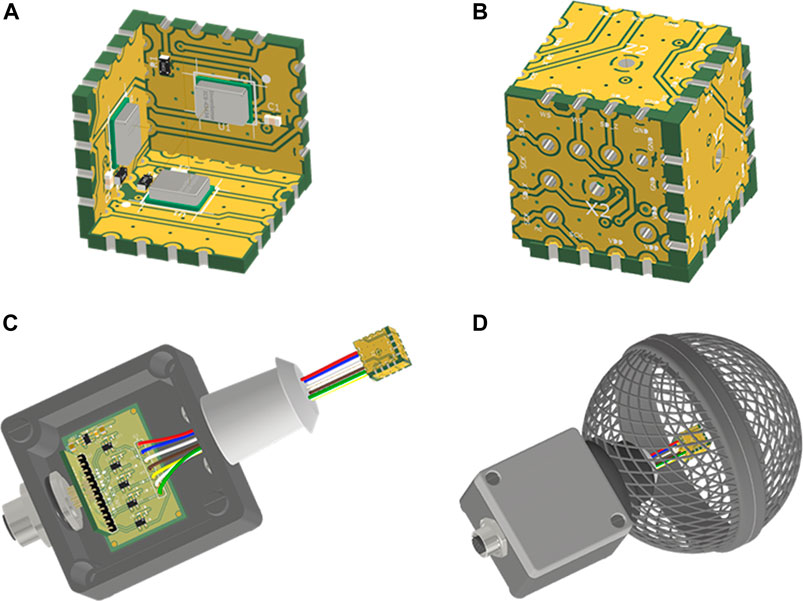
FIGURE 1. Acoustic probe: (A) interior view of the vector probe sensor, (B) complete vector probe sensor, (C) vector probe without windscreen, (D) complete vector probe.
The tiles are assembled in a cubic structure so that the pairs of microphones form the axes of a Cartesian system. The microphones communicate with the recording device via a digital interface I2S. The operating principle of the probe can be briefly described as follows. First, each microphone records an acoustic pressure signal.
The pressure difference between the microphones of each pair allows us to determine the pressure gradient and thus the vector representation of the acoustic velocity. The calculation of the acoustic intensity estimate consists in multiplying the acoustic velocity signal measured on a given axis by the averaged value of the acoustic pressure measured by all microphones and then integrating this product (which in the case of digital signals boils down to adding up the values from a given time interval). In the experiments, the integration period was assumed to be 256 samples at a sampling rate of 48 kHz, so the integration period is 125 ms and the resulting reading frequency is 187.5 Hz. The probe in question does not measure the physical magnitude of the intensity but only a quantity proportional to it. However, only the relative relationships between the intensity vectors are relevant. Therefore, it is sufficient to calculate the azimuth and elevation angles to determine the sound wave direction. Before the probe can be used for measurements, it has to be calibrated in an anechoic chamber, where the gain and phase of signals in individual microphone paths are corrected. The calibration was performed in our department at Gdańsk University of Technology (see Figure 2) (Kotus and Szwoch, 2018; Czyżewski et al., 2020).
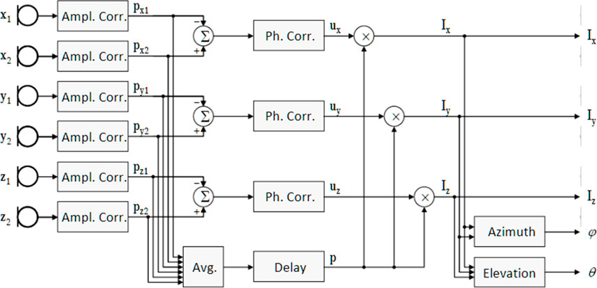
FIGURE 2. Block diagram of the signal processing algorithm of the acoustic intensity probe developed in Gdansk University of Technology (Kotus and Szwoch, 2018)
An experiment was conducted to record the sound emitted by the blades of a wind turbine. The place of recording was a wind farm located in Puck commune, Pomeranian voivodeship, in Poland. The recordings were made at relatively high wind speed. The intensity probe was mounted on a tripod at the height of approximately 1 m above the ground. The tripod was set on the back (leeward) side of an operating Nordex wind turbine (model N80, 2.5 MW), slightly to the left (approximately at an azimuth angle of 220° in the ground plane concerning the rotor position), at a distance of approximately 30 m from the tower (Figure 3). The coordinate probe system was set so that X-axis was directed vertically downwards, Y-axis - horizontally in the direction parallel to the turbine blades, Z-axis - horizontally towards the turbine. The probe signals were recorded on a laptop computer using Audacity software. Therefore, the following will only show the analysis results for the X and Z channel signals. The signal analysis was performed using scripts written in Python language.
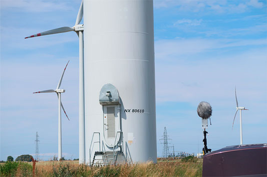
FIGURE 3. Intensity probe in the windshield during signal recording.
Figures 4A,B show the sound intensity waveforms measured in X (vertical) and Z (horizontal) directions. The calculated intensity signals were smoothed with the Sawicki-Golay filter of order 51 and degree 3 to remove the noise. The cyclic nature of the waveforms is apparent. Each local maximum occurs when air is cut by one of the rotor blades. The amplitudes of the waveforms are variable, likely due to fluctuations in wind speed. Although the waveforms for both directions have the opposite phase, there is also a slight, approximately constant shift between the minimum for the X-axis and the maximum for the Z-axis. The signal from X-axis (vertical) is characterized by significantly higher noise. Figure 4C shows a plot of the elevation angle calculated from the intensity signals from the X and Z axes. The cyclic nature of the waveform is also evident. The changes in the waveform values represent the movement of the apparent sound source, i.e., the turbine blades. The intervals between the maxima are approximately constant and describe the rotational motion of the turbine, but there are differences between the individual cycles.
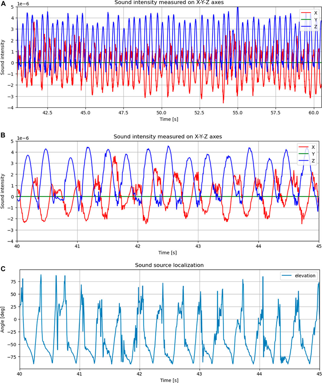
FIGURE 4. Acoustic intensity: (A) measured in directions X and Z, (B) enlargement of the fragment of the upper diagram, (C) the course of the elevation angle calculated from the intensity signals in the X and Z axes.
Figure 5 shows the spectrogram of the resulting sound intensity calculated in three dimensions (in this case, in two, due to lack of data for the Y channel). The spectrogram is a three-dimensional plot; the color intensity represents the amplitude of the spectral components (in linear scale) on the time-frequency plane and is made by calculating the signal spectrum in frames of 2048 samples with 75% overlap. In the graph, the effect of strong wind gusts on the recorded signals can be seen in components with high amplitude (green color) and low frequency (close to zero). These components cause rescaling of the graph and somewhat blur the fundamental intensity signal. However, a blurred waveform can be observed at a frequency of about 3 Hz. After searching for a spectral maximum in the range from 1.8 Hz (to remove the influence of noise) for each time frame and averaging this result, a value of 3.05 Hz was obtained, corresponding to a period of 328 ms. This value corresponds to the rotational speed of the turbine blades; a complete rotation cycle is approximately equal to 3 × 328 = 984 ms.
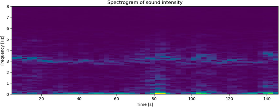
FIGURE 5. Spectrogram of the sound intensity.
Results of the experiments indicated the possibility of using an intensity probe to monitor the condition of a wind turbine. From the obtained intensity waveforms, it is possible to calculate the current rotational speed of the blades. More complex analyses are also possible. In the intensity and angle waveforms, every third maximum is caused by the same blade. Therefore, it is possible to select every third maximum for each blade from the run and average the readings over some time interval to remove the influence of variable wind speed. By comparing the readings obtained for each blade, an attempt can be made to detect blade damage if the results obtained for one blade are significantly different from the others. It is necessary to record signals from different wind turbines with varying levels of blade wear to perform experiments in this regard. It is also planned to record signals at different points in relation to the turbine to find the optimal measurement point and assess the influence of the probe position on the obtained results. It was also planned to use an intensity probe inside the nacelle to monitor the generator and detect irregularities in its operation. However, this issue requires separate experiments, described later in this paper.
4.2 Internal Analyser Concept
Realization of the SC2 measurement scenario, which assumes the monitoring of the wind turbine condition through sensors installed inside, requires physical access to the inside of the nacelle. For this purpose, access to the inside of the wind turbine nacelle located in Wydminy village was obtained. Wydminy is a village in Poland located in Warmińsko-Mazurskie Voivodeship, in Giżycko County, in Wydminy Commune. Installed wind turbines are 3 Fuhrländer FL MD 77, with a capacity of 1.5 MW each. The nacelle is installed at the height of 104 m. The rotor diameter is 77 m. The power plant starts working at a wind speed of 3 m/s. It obtains rated power at a wind speed exceeding 10 m/s. The maximum wind speed which ensures safe operation is 20 m/s. Above this speed, the emergency brake is activated.
The inspection of the inside of the nacelle was to obtain the information necessary to determine how to implement the SC2 scenario. The nacelle is equipped with an elevator (the trip to the top takes about 5 min). In addition, mechanical devices responsible for the production of electricity are installed on the upper deck of the nacelle. They include a slowly rotating shaft (to which the rotor is attached) with a set of bearings, gearbox, fast rotating shaft, power generator. These elements are critical components of the wind turbine, and their monitoring was performed as part of the SC2 measurement scenario.
4.2.1 Acoustic Analyzer Usage Scenarios
The basic scenario for using the proposed acoustic modality-based outdoor analyzer (SC1) is to install a noise monitoring station in the vicinity of the selected wind turbine. Once deployed, the station operates autonomously, performing continuous monitoring of acoustic signals. The acoustic signals are acquired using a selected acoustic sensor. The 3D intensity probe provides sound intensity signals. The sound intensity signal analysis complements the results of sound pressure analysis with information about the direction of the sound. Therefore, it is possible to locate the noise source and eliminate interference coming from directions other than the position of the analyzed wind turbine.
Due to the need to limit the volume of this article, the SC1 scenario is only hinted at, while in the following chapters, the analysis results presented will refer to the second scenario (SC2). For the internal measurement scenario (SC2), installing the equipment inside the nacelle is necessary.
5 Developed Measuring Station
The block diagram showing the concept of using the data acquisition module is shown in Figure 6A. The data acquisition module has a segmented structure, allowing multiplication (from 1 to max. 8) of two-channel signal transducers built into accelerometers. Thus, it is possible to obtain up to 16 channels. A single segment is 2-channel, can serve two accelerometers in the IEPE standard, and outputs an I2S digital signal in the form of two channels on a single signal line. A visualization of the modular measuring station is shown in Figure 6B.
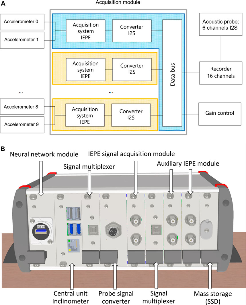
FIGURE 6. Data acquisition module: (A) block diagram, (B) module design. Some elements of the developed device prototypes are patent pending [41].
Software gain control is provided from −12 to 32 dB with 0.5 dB step. The control is implemented via an I2C serial interface using two lines from the Raspberry Pi computer. In addition, an I2C multiplexer electronic circuit is used to allow conflict-free addressing of the I2S converters. The 16-channel recorder is an MCH Streamer-type transmitter connected to the data-logging computer.
Two communication variants are provided for the measuring station, wired and wireless (over cellular networks). The station is also equipped with an SSD storage module. A 1 TB SSD disk was used as mass storage.
5.1 Artificial Intelligence Module
Neural networks have been successfully used for the classification of acoustic and video signals; however, their main drawback which hinders their practical application is the required considerable computational power at the stage of training and post-training of the network and less but significant computational power at the stage of inference and classification of data by the network.
A hybrid solution has been proposed by separating logically and physically the training and learning processes using mixed priorities (Figure 7). The system requires a central host unit and a dedicated neural coprocessor. The host CPU manages the system and performs acquisition, data recording, initial analysis, and parameterization, e.g., determination of the spectrogram of the acoustic signal. The training is conducted based on historical input data stored on disk, with low priority on the CPU, only when computational resources are available. Input classification is performed on live data acquired on a dedicated neural coprocessor, without latency and high priority. During training, the network states are stored in the main unit memory. The most accurate state, obtaining the smallest error value on validation data, is selected every fixed time interval. Then, an update of the network weights in the coprocessor is performed, and the training continues.
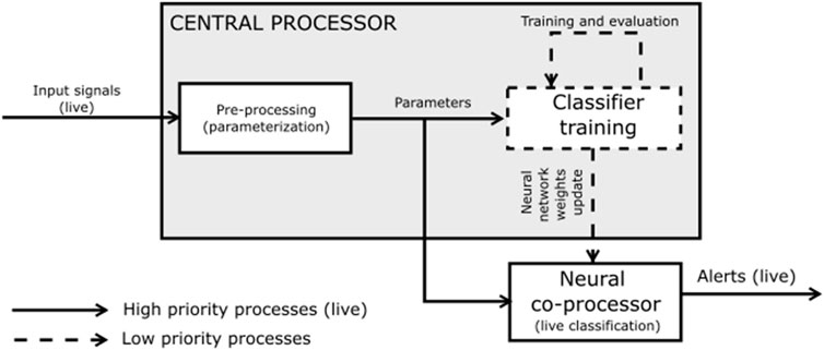
FIGURE 7. Block diagram of the hybrid host and neural coprocessor system for input data classification.
The described approach ensures optimized use of resources and minimal delays in response to input data, e.g., classification of threat situations recorded in the video and acoustic domain. However, in the research portion addressed in this paper, no neural network was trained for classifying signals. Therefore, this subject is deferred until the turbine is monitored for a long time until there are enough failures or signs of wear on the turbine mechanical components. However, since the autoencoder-type o neural network was used for feature extraction, thus this part of the system has already found a practical application.
5.2 Implementation and Startup of Autoencoder on Intel Compute Stick Platform
Running the solution on an embedded neural computing accelerator requires taking several steps to prepare the working environment. OpenVINO is a collection of software tools that enable developers of solutions based on artificial neural networks to run their designed networks on neural computing accelerators, including the Neural Compute Stick accelerator. The OpenVINO package also allows you to run optimized machine learning models on a CPU and other development platforms, a complete list of which can be found in the solution documentation (OpenVINO, 2022). Examples of such platforms are FPGAs, for example, or graphics cards.
The model used during inference can be computed using popular libraries Caffe or Tensorflow. For the experiment described in this report, model training was performed in the Tensorflow library version 2.0. It is a popular library for training neural networks. Still, for the use of such acquired machine learning models, it was necessary to convert the model format to that used in the TensorFlow library version 1.14. This is the format accepted by the OpenVINO software package. This conversion can be done by writing the raw model weights, e.g., to an HDF file (with h5 extension). Then it is possible to create the graph of the model in the library in the target version (TensorFlow 1.14) and perform the so-called freezing of the model.
In this way, the converted model, which is saved in an intermediate format (the file has the extension. pb), can then be processed by the optimization module of the OpenVINO package; When developing the neural network architecture, it is essential to keep in mind that, depending on the platform on which they will be run, some of the components that build neural networks may not be available. For example, in the case of networks described in this report, it was necessary to replace the layers performing one-dimensional splicing (Conv1D) with layers formally performing two-dimensional splicing (Conv2D), in which one of the dimensions was set to 1. Such a formal procedure was necessary because MYRIAD processor built-in Neural Compute Stick accelerator does not support the Conv1D layer. The process of preparing model files and running them using the inference engine is shown in Figure 8.
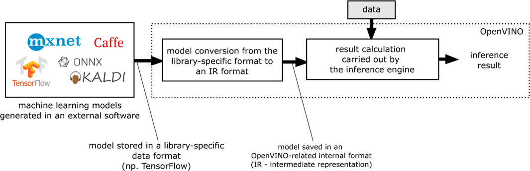
FIGURE 8. Schematic representation of successive model conversion steps from formats used by popular libraries for implementing machine learning algorithms to the internal format of the OpenVINO tool.
In addition, the execution time is measured. This was used to test the accelerator performance concerning computation on a virtual machine that has 8 GB of RAM allocated by software. The machine was run on a PC equipped with an AMD FX-8350 processor. PC calculators are the benchmark for calculations performed on the accelerator from the hardware platform developed within the project. The results of measuring the parameterization time of a single frame of a one-dimensional signal coming from sensors mounted on the turbine (see next section) are presented in Table 1.
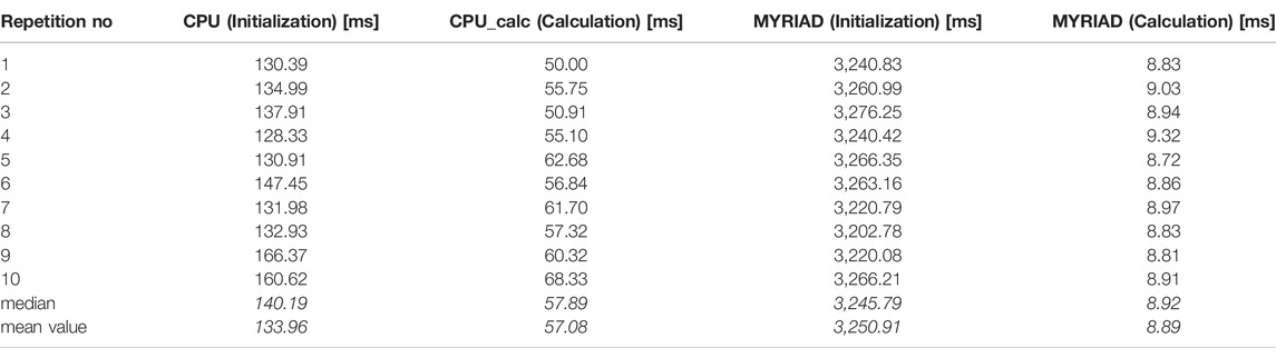
TABLE 1. Execution times of the inference procedure on the CPU and MYRIAD platforms. The times for loading the data into the VM memory or the Neural Compute Stick accelerator memory (the column: “initialization”) are also included.
Calculations performed with the accelerator were, on average, about 6.42 times faster than calculations using a CPU simulated in a virtual machine. The minimum cost-effective number of frames to compute with the accelerator was calculated using the following formula (Eq. 1):
where:
A model prepared and tested in this way is transferable between different types of inference engines, including the possibility of transferring the model to an engine developed with the Raspbian operating system. Furthermore, it is the preferred path for prototyping and applying machine learning models on a Raspberry PI board equipped with a neural computing accelerator.
6 Data Analysis
The sensors of the prototype recorder placed in the wind turbine are shown in Figure 9.
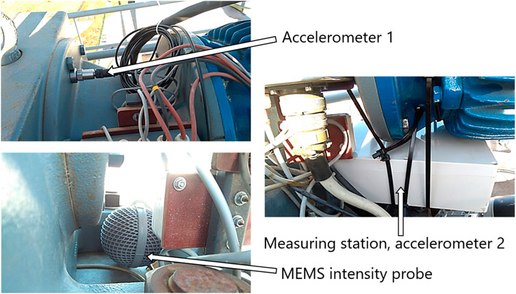
FIGURE 9. Sensors of the prototype recorder placed in the wind turbine (MEMS intensity probe means acoustic intensity sensor manufactured in micro-electro-mechanical, i.e., MEMS technology).
Measurement data were collected from a period of about 2 weeks, for each accelerometer a total of 308 h, for the intensity acoustic probe a total of 135 h. The stable operation of the turbine turned out to be relatively short throughout the time of continuous data recording, which was independent of the performed measurements and depended on the wind conditions. Therefore, the collected signals are characterized by a relatively small share of activity of the working mechanisms of the turbine, at the level of 15% of the whole time of data collection. The data were collected at a rate of 22 kSa/s with 16-bit resolution, and the intensity probe data at 48 kSa/s in six channels with 24-bit resolution.
6.1 Parameterization and Classification of Signals
For the research, the concept of a method for processing signals from sensors monitoring a wind turbine was developed. The first step is a data acquisition and source synchronization. The Mobile Measurement Station is responsible for these steps. Next, the parameterization is carried out, which consists in calculating two types of parameters: 1) from the time course of the signal and 2) from the spectral-time representation, i.e., the spectrogram. From the time signal, we get information about instantaneous amplitude, RMS value of the signal, frequency of transitions through zero, maximum amplitude. From spectrogram and FFT transforms information about spectral components and their changes in time, coefficients of FFT transform, mel-cepstral coefficients of MFCC transform (mel-frequency spectral coefficients).
The rationale for selecting the signal analysis method based on MFCC coefficients and autoencoders is its effectiveness proven in some previously known applications to noise analysis developed and tested with the author’s participation (Czyżewski et al., 2019).
The determination of MFCC coefficients is a multi-step procedure that is widely known from the literature, so it will not be described here (Zheng et al., 2001). However, it should be added that the research presented in this paper uses the first 40 MFCCs–20 first MFCC’s average values, 20 first MFCC’s variance values, and 20 delta MFCC and 20 delta-delta MFCC Coefficients. Using formula (2) it is possible to calculate the first and second-order derivatives of MFCC:
where
The parameters can be subjected to classification by selected methods such as: spline neural networks to process spectrograms, which are two-dimensional signals (time-frequency), and SVM classifiers, decision trees, or neural networks to process one-dimensional parameters vectors (amplitude, FFT, MFCC). In such a case, using a hardware accelerator (Intel Neural Compute Stick - NCS2 with Movidius chip) connected to a central unit in the Mobile Measurement Station for computations related to neural network inference is beneficial.
It is always expected that dedicated classifiers would efficiently classify a given period of turbine operation as typical or atypical and ascertain the degree of deviation from the nominal mode of operation (though regression). A concept of binary classifier operation is illustrated in Figure 10A.
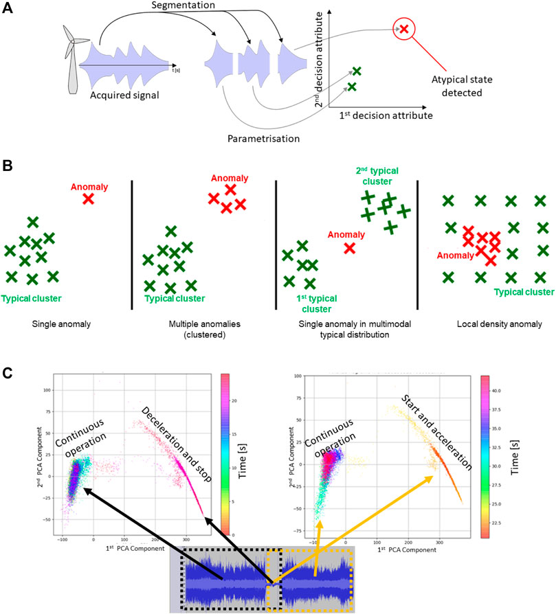
FIGURE 10. Concept of signal processing for deviation detection (A), examples of possible deviations from the standard (B), visualization of parameters obtained from the acoustic signal of the turbine (C).
A binary classifier that determines an atypical condition in a monitored device uses statistical dependencies to determine which of the measured parameters of the recorded signals should be considered typical and which significantly deviate from the expected values. It is assumed to use a hybrid combination of several approaches, including statistical and intelligent classifiers (e.g., neural networks and machine learning). The algorithm selected is intended to model statistical distributions of typical values (Figure 10B) and determine whether a new measurement deviates significantly from regular observations. Several types of deviations are possible: 1) a single anomaly or multiple anomalies clustered in the decision parameter space and significantly distant from the cluster (cluster) of typical values; 2) the occurrence of several clusters of typical values (e.g., associated with different regular turbine operating modes) and the observation of an anomaly significantly distant from each cluster.
Anomaly analysis can involve different types of parameter space. The type of parameters that form the basis of the analysis defines the arrangement of points and the sensitivity of the system to outliers in the general trends observed for the data as a whole. In the case of acoustic signals, MFCC parameters (mel-frequency cepstral coefficients) are applicable. They are characterized by the fact that they represent how acoustic stimuli are perceived by human hearing. Still, numerous studies have found them well suited for extracting the distinctive features of acoustic signals of various types for their automatic classification. Thus, this mechanism also works well in machine learning and acoustic signal classification tasks. The effect of parameterization of this type is the visualization of the course of a given phenomenon in the form of a system of points in the decision space. The initial high-dimensional decision space is helpful from the point of view of machine learning techniques used for target signal classification. On the other hand, visualization is helpful to visualize the test space using a dimensionality reduction technique such as PCA (Figure 10C).
In practice, unfortunately, a very rare phenomenon is the separation of individual states of the tested signal in the form of separate clusters. Instead, more subtle changes in the character of acoustic signals are often marked in the form of shifting locations of points related to a given period within one larger cluster. Such a tendency is illustrated in Figure 11, which shows the localization of individual states of the turbine activity on individual large clusters associated with the on and off state of the investigated turbine. Locating points in the decision space can define a distance metric between points and clusters of points. This type of metric, in turn, can form the basis for the definition of a classifier. It can be minimal-distance or probabilistic like mixed Gaussian models. In this type of case, clusters of points in the decision space computed from the source material are described by multivariate Gaussian distributions. The inference is then performed by determining the probability of the origin of new points from each of the determined clusters.
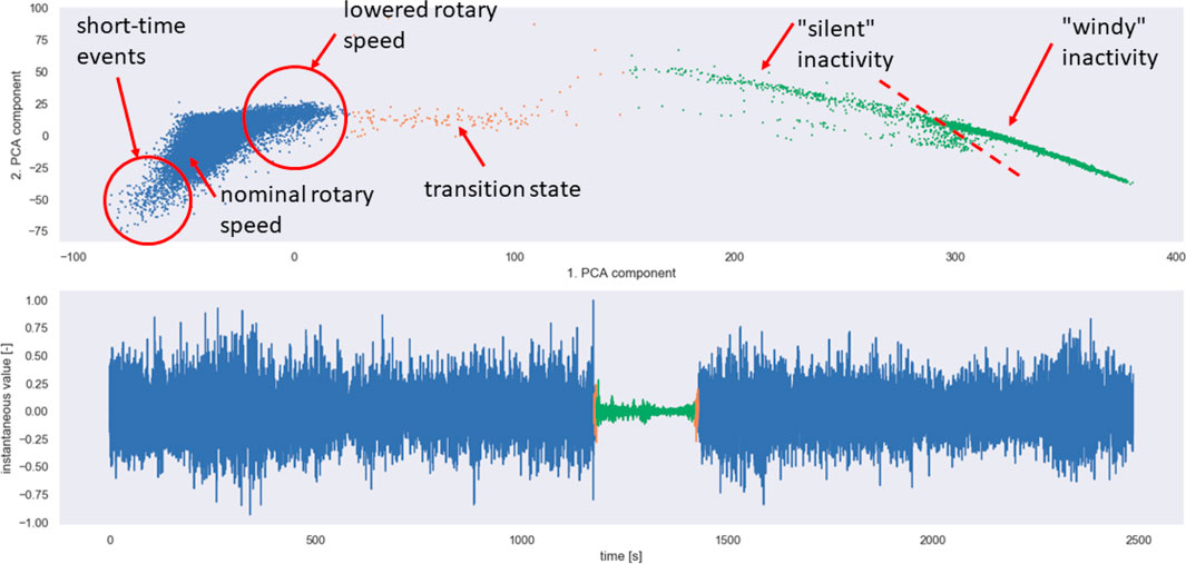
FIGURE 11. Illustration of wind turbine activity states in time course and parameter space, example of modeling the probability distribution of point placement based on its membership in a given class for operation under normal conditions, continuous operation, signals from the acoustic intensity probe.
Figures 12A,B show the results of parameterization of the audio signal recorded with the intensity probe (single channel in this case) using the discussed MFCC-PCA method. Groups of points characteristic of regular operation, anomalous operation, and abnormal situation are illustrated. The blue point cloud denotes the distribution in parameter space for the entire experiment, while the red points represent class-specific clusters. Figures 12C,D show the results of parameterization of the signal recorded with accelerometer one using the discussed MFCC-PCA method. Groups of points characteristics of regular operation, anomalous operation, and abnormal situation are illustrated. The blue point cloud indicates the distribution in parameter space for the whole experiment, while the red areas indicate the clusters characteristic of a particular class.
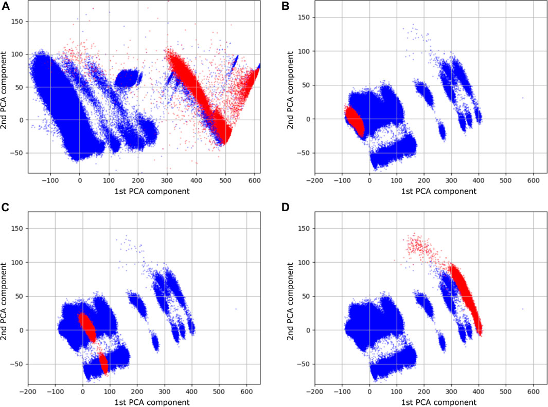
FIGURE 12. Operation under normal conditions, on/off - signals from the acoustic intensity probe (A), rotor deceleration - signals from acoustic intensity probe (B), continuous operation -signals from the accelerometer (C), on/off signals from the accelerometer (D).
Performed analyses of vibroacoustic damage data of wind generators showed that the proposed methods for analyzing data from multi-modal sensors of a mobile measurement station are suitable for use as classifiers of normal and abnormal states for this type of mechanism.
6.2 Parameterization Using an Autoencoder Neural Network
Parameterization can also be carried out based on other than statistic method allowing to take into account specificity of the signal acquired from monitored devices. An example of such a solution is a neural network with autoencoder architecture. An example of the general architecture of such a network is shown in Figure 13A. An autoencoder consists of two neural networks, an encoder, and a decoder. The encoder performs dimensionality reduction of multiple input modalities and represents them in the form of an n-element parameter vector, the so-called representation. The decoder is mainly used to learn the network - it reconstructs the signals of input modalities. The whole set of network-encoder and decoder is trained to make modality reconstruction errors as small as possible. The autoencoder with the encoder structure depicted in Figure 13B was used to analyze the signals from the turbines.
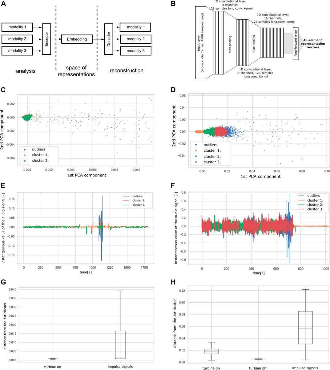
FIGURE 13. Neural network application: (A) the architecture of an autoencoder neural network, (B) autoencoder architecture used to analyze acoustic signals from wind turbines, (C) result of parameterization and signal clustering-visualization was obtained by parameter reduction with PCA method, (D) result of parameterization and clustering obtained by reducing the parameters with the PCA method, (E) and (F) results in the time domain, (G) and (H)-box plots illustrating the distance of points extracted from individual signal fragments from cluster 1.
The decoder had an analog (inverse) construction to the network encoder. A fragment of the signal was selected on which the correct operation of the device could be heard and a fragment in which the operation of the device was intentionally disturbed. The signal collected during the experiment had a sampling rate of 48 kSa/s. A half-hour fragment of normal work and a half-hour fragment of disturbing work were selected for calculations. These fragments were then divided into frames of 4,800 samples, corresponding to 100 ms at a sampling rate of 48 kSa/s. Thus, for both types of signal, 18,000 frames were obtained corresponding to successive fragments of the acoustic signal of 100 ms in length. An intensity acoustic probe recorded the acoustic signal. An autoencoder network fragment processed consecutive frames. After being split into frames and parameterized by the autoencoder neural network, the signal was subjected to a clustering process using the k average algorithm. The number of clusters k for the example with the fan was defined as k = 2. For the signal coming from the wind turbine, it was assumed that k = 3. The effects of such a clustering process are presented in Figure 13C and Figure 13D.
When analyzing the graphs in Figure 13C and Figure 13D, it is essential to keep in mind that the visualizations in the figures represent the effect obtained by dimensionality reduction (to visualize on the 2d plane of the graph). Therefore, clusters that are separable in high-dimensional space (40-dimensional in the case under consideration) do not always have to be visible as separate clusters in the visualization. However, the effect of separating separate clusters can be seen very clearly in Figure 13E Each point from the visualization is assigned to a single frame of the acoustic signal in temporal form. These frames have 4,800 samples, which corresponds to a length of 100 ms at a sampling rate of 48,000 Sa/s, which the analyzed recordings have.
The clustering effects transferred to the time domain are shown in Figure 13F. In the case of the signal from the actual turbine, the detection of outlier observations allowed the detection of impulsive signals in the recording. These were due to the clatter that occurred during the operation of the turbine. Additionally, clusters 2 and 3 correspond to the turbine on (running) state, with cluster 2 (green) corresponding to less intense operation and cluster 3 (red) to more intense operation. Finally, cluster 1 (orange) corresponds to the turbine shutdown state.
The final step was to check the statistical significance of the separation of the individual clusters. The standard level of significance was adopted
Student’s t-test was calculated to verify the statistical significance of the differences observed for the turbine signal. The statistic value of this test is equal to 19.3. The associated p-value is less than
In the case of the turbine signal, it was necessary to use a statistical test to compare three groups of distances. The results of tests for normality of distance distributions were characterized by p-values smaller than
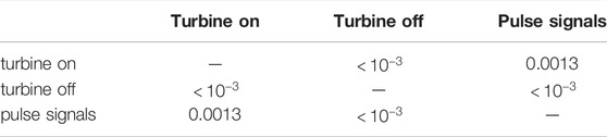
TABLE 2. Results of Dunn post-hoc test in the form of p-value table. Assuming the level of significance
7 Conclusion
The constructed measuring station and its application in monitoring wind turbines were described in the paper. An engineered acoustic intensity probe was used in addition to accelerometers. Therefore, multi-way monitoring of the turbine mechanism performance became possible.
As it was said in Chapter 6, measurement data were collected from a period of about 2 weeks, for each accelerometer a total of 308 h, for the intensity acoustic probe a total of 135 h. Unfortunately, we do not yet have multi-year data for machine learning at the current stage of the project development, which has made it impossible to apply deep learning methods at the present stage. Still, the results are promising, as the described research has demonstrated the correctness of the signal acquisition system in the conditions prevailing in the wind turbine and the effectiveness of the proposed data analysis method.
The MFCC coefficients (mel-frequency spectral coefficients) were used to represent acquired signals. An autoencoder-type neural network is also an alternative solution for feature extraction. In this case, we do not have to calculate MFCC coefficients. Still, we rely on the automatic operation of the autoencoder, which reduces given frames of signal samples to the parameterized form. This is a second way to show and investigate outlier observations.
The algorithm was designed for unsupervised (autonomous) training to identify statistically significantly different parameter values clusters. These clusters are interpreted in practice as periods of typical operation of the monitored device and abnormal events.
The graphs depicting the condition of the monitored wind turbine are interesting. They allow us to detect disturbing changes in noise that were registered. Still, the algorithm created separate clusters associated with periods of more and less intense turbine operation for the period when the turbine was on. Therefore, it is possible to assume that this solution may be suitable for automatic monitoring of the correct operation of wind turbine mechanisms, especially bearings, shafts, and gears.
Prospective work may involve analyzing data collected over an appropriate (very long) period to detect and describe temporal changes in cluster characteristics related to the in-service wear of powertrain components. As the components of the device wear out over several months and years, the parameters determined from the signal will change, affecting the displacement of values in the clusters. Applying even more sophisticated methods to interpret outlier observations and model turbine operating states will become possible, including mixed Gaussian mixture algorithms at the signal parameterization stage and deep learning in classification. It is planned for the future when the system will collect data from such a lengthy operation that a significant number of abnormal states of the turbine caused by wear or damage of its mechanisms might occur.
Data Availability Statement
The original contributions presented in the study are included in the article/Supplementary Materials, further inquiries can be directed to the corresponding author.
Author Contributions
AC designed the research, participated in the engineering and experimental work performed by the team he led, and described the results obtained in this article.
Funding
Project STEO - System for Technical and Economic Optimization of Distributed Renewable Energy Sources, No. POIR.01.02.00-00-0357/16 contracted by VIS Energia sp. z. o. o. is co-financed by the National Centre for Research and Development from the European Regional Fund.
Conflict of Interest
The author declares that the research was conducted in the absence of any commercial or financial relationships that could be construed as a potential conflict of interest.
Publisher’s Note
All claims expressed in this article are solely those of the authors and do not necessarily represent those of their affiliated organizations, or those of the publisher, the editors and the reviewers. Any product that may be evaluated in this article, or claim that may be made by its manufacturer, is not guaranteed or endorsed by the publisher.
Acknowledgments
I would like to express my indebtedness to my colleagues belonging to the team led by me, who made this extensive project possible. In particular, I would like to thank two team members, namely Grzegorz Szwoch, for the literature review he conducted and Adam Kurowski for performing the analyses illustrated in some figures in Chapter 6. In addition, my appreciation goes to my Ph.D. student Andrzej Sroczyński for constructing the measuring station.
References
Bechhoefer, E., and Kingsley, M. (2009). A Review of Time Synchronous Average Algorithms. San Diego, USA: Annual Conference of the Prognostics and Health Management Society. Available at: https://papers.phmsociety.org/index.php/phmconf/article/view/1666 (Accessed January 15, 2022).
Bouzid, O. M., Tian, G. Y., Cumanan, K., and Moore, D. (2015). Structural Health Monitoring of Wind Turbine Blades: Acoustic Source Localization Using Wireless Sensor Networks. J. Sensors 2015, 139695. doi:10.1155/2015/139695
Bowdler, D. (2008). Amplitude Modulation of Wind Turbine Noise. A Review of the Evidence. Acoust. Bull. 33 (4), 31–35.
Brüel & Kjaer Vibro (2014). Envelope Analysis for Effective Rolling-Element Bearing Fault Detection – Fact or Fiction? Application Note BAN0024-EN-11, https://www.bkvibro.com/fileadmin/mediapool/Internet/Application_Notes/BAN0024EN12_TD_Envelope.pdf.
Castellani, F., Garibaldi, L., Daga, A. P., Astolfi, D., and Natili, F. (2020). Diagnosis of Faulty Wind Turbine Bearings Using Tower Vibration Measurements. Energies 13 (6), 1474. doi:10.3390/en13061474
Coronado, D., and Fischer, K. (2015). Condition Monitoring of Wind Turbines: State of the art., User Experience and Recommendations. Bremerhaven, Germany: Fraunhofer Institute for Wind Energy and Energy System Technology IWES. Project report. Available at: http://publica.fraunhofer.de/documents/N-352558.html (Accessed January 15, 2022).
Cui, Y., Bangalore, P., and Tjernberg, L. B. (2018). “An Anomaly Detection Approach Based on Machine Learning and SCADA Data for Condition Monitoring of Wind Turbines,” in 2018 IEEE International Conference on Probabilistic Methods Applied to Power Systems (PMAPS), Boise, ID, USA, 24-28 June 2018, 1–6. doi:10.1109/pmaps.2018.8440525
Cygert, S., and Czyzewski, A. (2018). Eulerian Motion Magnification Applied to Structural Health Monitoring of Wind Turbines. J. Acoust. Soc. Am. 144, 1796. doi:10.1121/1.5067923
Czyżewski, A. (2019). Diagnosing Wind Turbine Condition Employing a Neural Network to the Analysis of Vibroacoustic Signals. J. Acoust. Soc. Am. 146 (4), 2952. doi:10.1121/1.5137251
Czyżewski, A., Kotus, J., and Szwoch, G. (2020). Estimating Traffic Intensity Employing Passive Acoustic Radar and Enhanced Microwave Doppler Radar Sensor. Remote Sens. 12 (1), 110. doi:10.3390/rs12010110
Czyżewski, A., Kotus, J., and Szwoch, G. (2021). Intensity Probe with Correction System. Warsaw: Polish Patent Office. Polish patent No. 236718.
Czyżewski, A., Kurowski, A., and Zaporowski, Sz. (2019). Application of Autoencoder to Traffic Noise Analysis. J. Acoust. Soc. Am. 146 (4), 2958. doi:10.1121/1.5137275
Deshmukh, S., Bhattacharya, S., Jain, A., and Paul, A. R. (2019). Wind Turbine Noise and its Mitigation Techniques: A Review. Energy Procedia 160, 633–640. doi:10.1016/j.egypro.2019.02.215
Fazenda, B. M., and Comboni, C. (2012). “Acoustic Condition Monitoring of Wind Turbines: Tip Faults,” in The 9th International Conference on Condition Monitoring and Machinery Failure Prevention Technologies, London, 12-14 Jun 2012. http://usir.salford.ac.uk/27344/.
Fuentes, R., Dwyer-Joyce, R. S., Marshall, M. B., Wheals, J., and Cross, E. J. (2020). Detection of Sub-surface Damage in Wind Turbine Bearings Using Acoustic Emissions and Probabilistic Modelling. Renew. Energy 147 (part 1), 776–797. doi:10.1016/j.renene.2019.08.019
García Márquez, F. P., Tobias, A. M., Pinar Pérez, J. M., and Papaelias, M. (2012). Condition Monitoring of Wind Turbines: Techniques and Methods. Renew. Energy 46, 169–178. doi:10.1016/j.renene.2012.03.003
Gellermann, T. (2013). Extension of the Scope of Condition Monitoring Systems for Multi-MW and Offshore Wind Turbines. VGB Power Tech J. 09.
Germanischer Lloyd (2018). Service Specification. GL Renewables Certification: Guideline for the Certification of Wind Turbines. Available at: https://wordpressstorageaccount.blob.core.windows.net/wp-media/wp-content/uploads/sites/649/2018/05/Session_3_-_Handout_3_-_GL_Guideline_for_the_Certification_of_Wind_Turbines.pdf (Accessed January 15, 2022).
Hameed, Z., Hong, Y.S., Cho, Y.M., Ahn, S.H., and Song, C.K. (2009). Condition Monitoring and Fault Detection of Wind Turbines and Related Algorithms: a Review. Renew. Sustain. Energy Rev. 13, 1–39. doi:10.1016/j.rser.2007.05.008
International Standard ISO 13373-1 (2002). Condition Monitoring and Diagnostics of Machines — Vibration Condition Monitoring.
International Standard ISO 13373-2 (2016). Condition Monitoring and Diagnostics of Machines - Vibration Condition Monitoring -- Part 2: Processing, Analysis and Presentation of Vibration Data.
International Standard ISO 13379-1 (2012). Condition Monitoring and Diagnostics of Machines — Data Interpretation and Diagnostics Techniques – General Guidelines.
International Standard ISO 61400-25-6 (2010). Communication for Monitoring and Control of Wind Power Plants - Logical Node Classes and Data Classes for Condition Monitoring.
Kotus, J., and Szwoch, G. (2018). Calibration of Acoustic Vector Sensor Based on MEMS Microphones for DOA Estimation. Appl. Acoust. 141, 307–321. doi:10.1016/j.apacoust.2018.07.025
Luo, H., Hatch, C., Kalb, M., Hanna, J., Weiss, A., and Sheng, S. (2013). Effective and Accurate Approaches for Wind Turbine Gearbox Condition Monitoring. Wind Energy 17, 715–728. doi:10.1002/we.1595
Mollasalehi, E., Wood, D., and Sun, Q. (2017). Indicative Fault Diagnosis of Wind Turbine Generator Bearings Using Tower Sound and Vibration. Energies 10, 1853. doi:10.3390/en10111853
Naumann, J. R. (2016). Acoustic Emission Monitoring of Wind Turbine Bearings (Univ. of Sheffield). Ph.D. thesis. http://etheses.whiterose.ac.uk/12397/1/JN%20Thesis%2016.12.2015.pdf (Accessed January 15, 2022).
Oerlemans, S. (2011a). An Explanation for Enhanced Amplitude Modulation of Wind Turbine Noise. National Aerospace Laboratory, report no. NLR-TP-2011-071. Available at: http://www.ref.org.uk/Files/RUK-A1.pdf (Accessed January 15, 2022).
Oerlemans, S. (2011b). Wind Turbine Noise: Primary Noise Sources. National Aerospace Laboratory, report no. NLR-TP-2011-066. Available at: https://reports.nlr.nl/xmlui/handle/10921/117 (Accessed January 15, 2022).
Okada, Y., Yoshihisa, K., Higashi, K., and Nishimura, N. (2015). Radiation Characteristics of Noise Generated from a Wind Turbine. Acoust. Sci. Tech. 36 (5), 419–427. doi:10.1250/ast.36.419
OpenVINO (2022). OpenVINO™ - an Open-Source Toolkit for Optimizing and Deploying AI Inference. Available at: https://docs.openvino.ai/latest/index.html (Accessed January 15, 2022).
Papasalouros, D., Tsopelas, N., Anastasopoulos, A., Kourousis, D., Lekou, D. J., and Mouzakis, F. (2013). Acoustic Emission Monitoring of Composite Blade of NM48/750 NEG-MICON Wind Turbine. J. Acoust. Emiss. 31, 36–49.
Pedregal, D. J., García, F. P., and Roberts, C. (2009). An Algorithmic Approach for Maintenance Management Based on Advanced State Space Systems and Harmonic Regressions. Ann. Oper. Res. 166, 109–124. doi:10.1007/s10479-008-0403-5
RenewableUK (2013). Wind Turbine Amplitude Modulation: Research to Improve Understanding as to its Cause and Effect, Industry Statement on OAM. Available at: https://www.renewableuk.com/page/IndustryStatementOAM (Accessed January 15, 2022).
Rogers, A. L., Manwell, J. F., and Wright, A. (2002). Wind Turbine Acoustic Noise. A white paper prepared by the Renewable Energy Research Laboratory Department of Mechanical and Industrial Engineering University of Massachusetts at Amherst, Available at: http://www.proj6.turbo.pl/upload/file/424.pdf (Accessed January 15, 2022).
Sheng, S. (2012) Wind Turbine Gearbox Condition Monitoring Round Robin Study - Vibration Analysis. Technical Report. https://dx.doi.org/10.2172/1048981.
Siegel, D., Zhao, W., Lapira, E., AbuAli, M., and Lee, J, (2014). A Comparative Study on Vibration-Based Condition Monitoring Algorithms for Wind Turbine Drive Trains. Wind Energy 17 (5), 695–714. doi:10.1002/we.1585
Sokołowski, P., Cygert, S., and Szczodrak, M. (2019). “Wind Turbines Modeling as the Tool for Developing Algorithms of Processing Their Video Recordings,” in 2019 Signal Processing: Algorithms, Architectures, Arrangements, and Applications (SPA), Poznań, Poland, 18-20 Sept. 2019. doi:10.23919/spa.2019.8936801
Stetco, A., Dinmohammadi, F., Zhao, X., Robu, V., Flynn, D., Barnes, M., et al. (2019). Machine Learning Methods for Wind Turbine Condition Monitoring:A Review. Renew. Energy 133, 620–635. doi:10.1016/j.renene.2018.10.047
Teng, W. (2021). Vibration Analysis for Fault Detection of Wind Turbine Drivetrains—A Comprehensive Investigation (2021). Sensors 21 (5), 1686. doi:10.3390/s21051686
Van Dam, J. V., and Bond, L. J. (2015). “Acoustic Emission Monitoring of Wind Turbine Blades,” in SPIE Proceedings,Smart Materials and Nondestructive Evaluation for Energy Systems 2015, 94390C. doi:10.1117/12.2084527
Wang, W., and McFadden, P. (1996). Application of Wavelets to Gearbox Vibration Signals for Fault Detection. J. Sound Vib. 192 (5), 927–939. doi:10.1006/jsvi.1996.0226
Wismer, N. (1994). Application Note: Gearbox Analysis Using Cepstrum Analysis and Comp Liftering. Denmark: Brüel & Kjaer. Available at: https://pearl-hifi.com/06_Lit_Archive/15_Mfrs_Publications/10_Bruel_Kjaer/04_App_Notes/Cepstrum_Analysis_Gearbox.pdf (Accessed January 15, 2022).
Keywords: wind turbines, remote monitoring, acoustic intensity, accelerometers, machine learning, neural networks, autoencoders
Citation: Czyżewski A (2022) Remote Health Monitoring of Wind Turbines Employing Vibroacoustic Transducers and Autoencoders. Front. Energy Res. 10:858958. doi: 10.3389/fenrg.2022.858958
Received: 20 January 2022; Accepted: 29 March 2022;
Published: 10 May 2022.
Edited by:
Yolanda Vidal, Universitat Politecnica de Catalunya, SpainReviewed by:
Davide Astolfi, University of Perugia, ItalyFrancesc Pozo, Universitat Politecnica de Catalunya, Spain
Copyright © 2022 Czyżewski. This is an open-access article distributed under the terms of the Creative Commons Attribution License (CC BY). The use, distribution or reproduction in other forums is permitted, provided the original author(s) and the copyright owner(s) are credited and that the original publication in this journal is cited, in accordance with accepted academic practice. No use, distribution or reproduction is permitted which does not comply with these terms.
*Correspondence: Andrzej Czyżewski, YWNAcGcuZWR1LnBs