Geologic Modeling and Ensemble-Based History Matching for Evaluating CO2 Sequestration Potential in Point bar Reservoirs

1 Introduction

Point bars are fluvial deposits formed at the inner bend of a meandering channel by erosion of channel sediments at the outside of a meandering channel (i.e., cutbank) and deposition of the eroded sediments at the inner bend of the meander (Willis & Tang, 2010). Point bar reservoirs have significant storage capacity. For example, the Athabasca Oil Sands deposit in the Lower Cretaceous McMurray Formation—which hosts one of the world’s largest heavy oil accumulations—is predominantly composed of point bar deposits (Labrecque et al., 2011; Austin-Adigio et al., 2018). Also, The Cranfield, Mississippi reservoir which is considered by several studies (e.g., Daley et al., 2014; Delshad et al., 2013; Lu et al., 2013a; Yang et al., 2013; Zhang et al., 2013) as a viable candidate for CO₂ sequestration experiments is largely composed of a point bar deposit. However, point bars exhibit a high level of spatial heterogeneity (Su, et al., 2013). These heterogeneities interrupt reservoir connectivity and impede fluid flow, which then affects the distribution of fluids and the recovery efficiency of recovery schemes in point bar reservoirs (Davies and Haldorsen, 1987; Stephen, et al., 2001). Developing a geologically realistic modeling framework for representing point bar heterogeneities, as well as implementing a data assimilation procedure for calibrating the model is essential.

In point bar modeling, data from outcrop analogs have been used (e.g., Pranter et al., 2007; Musial et al., 2013) to predict and model the internal heterogeneities (e.g., shale drapes). However, outcrop-based models may not reflect subsurface conditions because the details of the heterogeneities may not be preserved in the outcrop sections (Nardin et al., 2013). Therefore, the use of outcrop-based models may result in an inaccurate prediction of process performance such as injection of CO₂ for subsurface sequestration.

Other methods have been proposed for improving the modeling of point bar reservoirs. Examples of such methods include object-based methods (e.g., Deutsch & Wang, 1996; Deutsch and Tran, 2002; Deutsch & Tran, 2002; Boisvert, 2011; Yin, 2013), process-based methods (e.g., Pyrcz, 2001; Pyrcz and Deutsch, 2004; Pyrcz et al., 2009; Shu et al., 2015), surface-based methods (e.g., Pyrcz et al., 2005; Niu et al., 2021) and geostatistical simulation methods (e.g., Sequential Indicator Simulation (Deutsch, 2006)).

Of all these methods, geostatistical simulation methods remain popular among modelers. The geostatistical methods use statistical measures such as semi-variograms or multiple point statistics to describe the spatial continuity of reservoir rocks. These methods are very useful in situations where there is good knowledge about the typical spatial variability observed in such reservoir albeit with conditioning data. However, heterogeneities exhibited by complex reservoir geometries such as in point bars can be destroyed during the modeling process. The reason is that, most geostatistical methods (whether variogram-based methods (e.g., Gringarten and Deutsch, 1999) or multiple-point statistical methods (e.g., Caers and Zhang, 2005; Eskandari and Srinivasan, 2018)) rely on regular grids (and templates) to model spatial continuities. Therefore, they are of limited use for modeling spatial heterogeneity such as those introduced by erosional and truncation surfaces (Li and Srinivasan, 2015).

The methods discussed thus far, have fostered developments in point bar reservoir modeling; however, the use of these methods in workflows to assess the displacement of CO₂ plume and calibration of point bar reservoir models is, at best, rare. Therefore, a systematic workflow is necessary to improve the geologic modeling process, to ensure a reliable study of the CO₂ sequestration potential in point bar reservoirs.

This study is in two parts; in the first part, we propose a geologic modeling approach that honors the curvilinear geometry and heterogeneities of point bars. The preservation of point bar geometry and heterogeneities is achieved by 1) implementation of a gridding scheme that generates high quality curvilinear grids representative of the point bar geometry, 2) incorporation of an appropriate grid transformation scheme in the geostatistical simulation process.

In the second part of this study, the point bar reservoir model is history matched (i.e., calibrated) to reflect the observed CO₂ injection data. This step is necessary as it reduces the uncertainty in the geologic model for a reliable assessment and prediction of the CO₂ sequestration potential of the point bar reservoir. The entire workflow in this study is implemented on a dataset from the Cranfield in Mississippi, which is a large scale storage site for CO₂ sequestration (Hovorka, et al., 2013). In the model calibration procedure, we take into account the fact that: 1) the reservoir geometry exerts important controls on fluid flow (e.g., Willis and White, 2000; Pranter et al., 2007; Deveugle et al., 2011), and therefore needs to be constrained, and 2) the petrophysical property distribution in the point bar reservoir is likely to be non-Gaussian, given the depositional trends and the complex spatial structure of the Cranfield reservoir geology as described in previous works (e.g., Lu et al., 2013). In response to these considerations, a two-step ensemble-based data assimilation procedure is used in the model calibration. For step 1, ensemble Kalman filter (EnKF) is used to update ensembles of point bar reservoir model geometries (e.g., the shape of the IHS surfaces etc.), to select the geometry that yields the closest match to observed data. For step 2, Indicator-based data assimilation (InDA) is adapted to update ensembles of spatially distributed permeabilities within the optimal reservoir geometry as determined in step1. The indicator-based model updating scheme does not presume Gaussianity of the property distribution.

1.1 Point Bar Reservoir Heterogeneities

The heterogeneities and depositional trends in point bars have stimulated several scholarly contributions among researchers and modelers (e.g., Allen, 1964, Allen, 1965, Allen, 1970; Visher, 1964; Thomaset al., 1987). The heterogeneities are formed by episodic migration of sinuous channels, which leads to erosion and deposition of channel sediments. Several periodic lateral accretions are prominent patterns that are observed in point bars (Ghazi & Mountney, 2009; Miall, 1988). The lateral accretions define the aerial dimensions of the heterogeneities while the inclined heterolithic stratifications (IHS) define the vertical dimensions (see Figure 1A). Within point bars, a fining upward trend is common. Sand-prone sediments dominate the bottom of the sequence and transition to silt-prone and mud-prone sediments at the top (Thomas et al., 1987; Labrecque et al., 2011; Fustic et al., 2012). In the past, research studies (e.g., Li and White, 2003; Yue and Shiyue, 2016; Sun et al., 2017) have shown that the lateral accretions (and IHS) constitute the most important heterogeneities that influence fluid flow in point bar systems. This is because of the shale drapes that occur along the surfaces of the lateral accretions and the IHS. The shale drapes are potential flow baffles (Richardson et al., 1978; Hartkamp-Bakker and Donselaar, 1993); they compartmentalize the point bar reservoir and greatly reduce CO₂ storage capacity of the point bar (Issautier et al., 2013; Issautier et al., 2014). In this study, we will make an attempt to represent these heterogeneities in the geological model of the point bar.

FIGURE 1

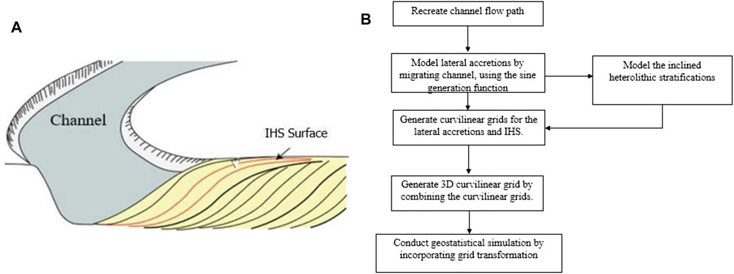
FIGURE 1. (A) point bar schematic showing laterally accreating sigmoidal inclined heterolithic surfaces, as adapted from (McMahon and Davies, 2018), and (B) workflow for modeling point bar reservoir geometry and petrophysical properties.

2 Methodology

2.1 Geological Model Construction

The geological modeling process basically involves recreating the channel flow path and its subsequent migration. The heterogeneities are gridded separately and combined to form a 3D point bar grid. Finally, the point bar property distribution is modeled within the gridded geometry using geostatistical simulation, by incorporating a grid transformation scheme. Figure 1B summarizes the workflow for modeling the point bar reservoir.

2.1.1 Geometric Modeling of the IHS and Lateral Accretions

The IHS surfaces are typically modeled as approximately sigmoidal surfaces (Thomas et al., 1987) (see Figure 1A). Accordingly, we modeled the geometry of the IHS using a sigmoidal function defined as:

$f=\frac{h}{1+e^{-ax}}(1)$

where $h$ is the vertical thickness of the point bar and $a$ controls the slope of the IHS over a horizontal distance $x$. The lateral accretions were modeled by approximating the meandering channel path with a sine generation function (SGF). The SGF describes the most probabilistic path defined by the channel as it migrates, and it is based on the idea that the direction angle along the channel path changes sinusoidally (Hathout, 2015). The original SGF as proposed by (Langbein and Leopold, 1966) is in radial coordinates. In this study, we will work in Cartesian coordinates, therefore, the parametric forms of the SGF (Movshovitz-Hadar and Shmukler, 2000; Hathout, 2015) will be used (see Eqs 2a, 2b).

$x\left(t\right)={\displaystyle \underset{0}{\overset{t}{\int }}\cos \left[\omega \cdot \sin \left(\frac{2\pi l}{L}\right)\right]dl}(\mathrm{2a})$

$y\left(t\right)={\displaystyle \underset{0}{\overset{t}{\int }}\sin \left[\omega \cdot \sin \left(\frac{2\pi l}{L}\right)\right]dl}(\mathrm{2b})$

where ⍵ is the maximum angular displacement of the channel with the horizontal; $0^{\circ }<\omega <{90}^{\circ }$; $l$ is the length at any point along the channel; $0<t<L$ and the total length of the channel, $L$, can be approximated numerically by dividing the channel path into $n$ subintervals to generate $P$ points, so that $L$ becomes:

$\text{L}=\underset{\text{n}\to \infty }{\lim }{\displaystyle \sum }_{\text{i}=1}^{\text{n}}|{\text{P}}_{\text{i}+1}-{\text{P}}_{\text{i}}|(\mathrm{2c})$

2.1.2 Channel Path Recreation

To model the heterogeneities, it is necessary to recreate the channel flow path conditioned to well data. Based on well logs, the facies are grouped into channel facies and point bar facies. In previous works (e.g., Odundun and Nton, 2011; Nazeer et al., 2016), SP logs have been used to infer channel and point bar facies, where a bell shape signal has been interpreted as a point bar while a blocky or cylindrical shape has been interpreted as a channel (see Figure 2A). In this study, SP logs from the Cranfield dataset were used for facies interpretation. Figures 2B,C show some of the wells (31-F1 and 48-2) used in this study and how the facies interpretation was done.

FIGURE 2

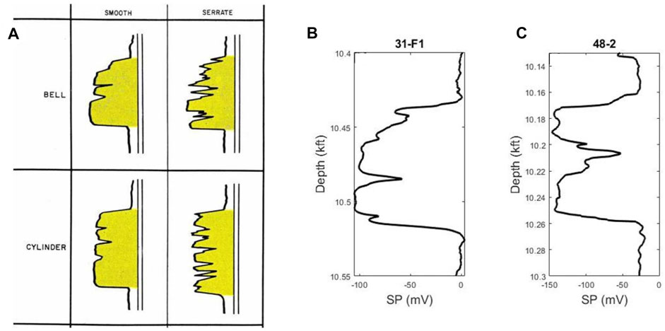
FIGURE 2. Facies identification from SP log. (A) Typical SP log signatures for point bars (bell shape) and channels (cylindrical shape), as adapted from (Wilson and Nanz, 1959), (B) point bar and (C) channel facies identified from SP log readings for wells31-F1 and 48-2, using the Cranfield dataset. shale breaks, typefied by sudden increase in SP logs readings are prominent trends observed for the Cranfield reservoir geology.

The workflow for channel path recreation is as summarized in Figure 3. In modeling stage 1 (Figure 3A), the facies are grouped into point bars and channels, based on well logs. All the blue points are channel well locations and the red ones are point bar locations. We then sort the facies in the direction of the channel flow path, which is in the NW-SE direction (Olulana, 2015). In modeling stage 2 (Figure 3B), the channel path recreation begins. The channel path is conditioned to go through the channel locations sequentially and bend to accommodate the point bar locations on the concave side of the bend. This is consistent with the formation of point bars at the inner bends of the channel meanders during lateral migration. In modeling stage 2, the channel path should have progressed from channel node two to channel node three; but in that case, the channel path will not be able to bend to accommodate the point bar at location one on the concave side of the bend. In situations such as this, secondary nodes are inserted to guide the channel path. From there onwards, the channel path follows the channel nodes sequentially until all the well data is accommodated, as illustrated in stage 4 (Figure 3D). The encircled region in the last modeling stage (Figure 3D) is the Detailed Area of Study (DAS), which is the CO₂ injection site at Cranfield in Mississippi. This area would be selected for developing the detailed model of the point bar.

FIGURE 3

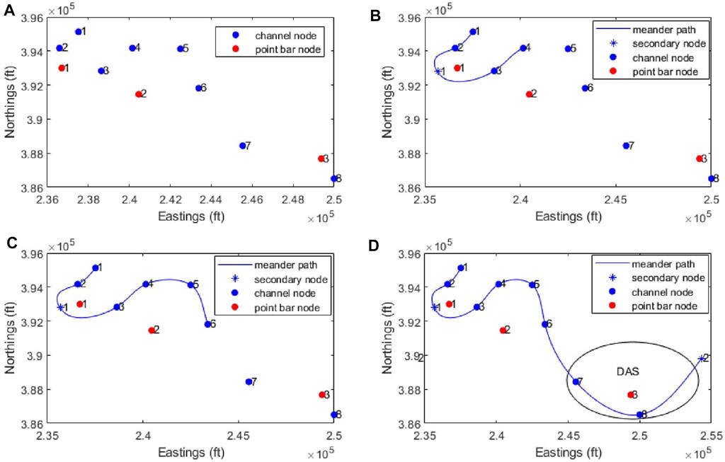
FIGURE 3. Channel path simulation for the Cranfield dataset, (A) Modelling stage 1-Locations for the point bar (red) and channel facies (blue) interpreted using SP logs, (B) Modelling stage 2-channel path recreation begins. secondary node is inserted to guide the channel path, (C) Modelling stage 3 and (D) final Modelling stage-channel path follows the channel nodes sequentially until all the well data is accommodated. The circled area in the final figure is the Detailed Area of Study(DAS) at the Cranfield injection site.

2.1.3 Meander Path Migration

Migrating the current channel path back in time to recreate the initial channel path allows us to capture the geometry of lateral accretions. The channel path in the DAS in Figure 3D is approximated using the SGF. As can be seen in Figure 4A, the SGF gives a close approximation of the original channel path; this confirms earlier reports by (Langbein and Leopold, 1966; Hathout, 2015). The backward migration of the channel is done by decreasing the angular placement (⍵) in the SGF to recreate the initial channel path (see Figure 4B; arrow indicates the direction of backward migration). The corresponding vertical heterogeneities are modeled, such that any section across the channel paths as done in Figure 4C displays the IHS as illustrated in Figure 4D.

FIGURE 4

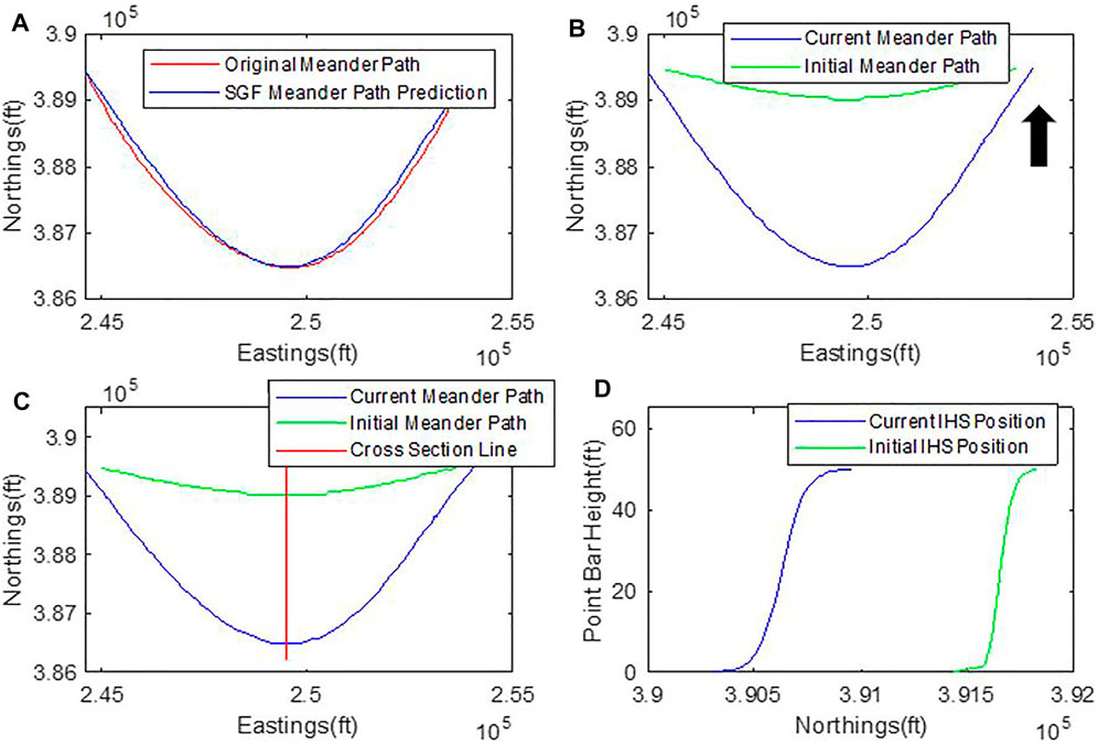
FIGURE 4. Meander migration process. (A) Illustration of close match between SGF prediction and the original meander path, (B) Current and initial meander path location after backward migration of channel (arrow indicates direction of backward migration, i.e., migration starting from today’s channel path to the ancient path), red line shows section across the meanders, and (D) IHS revealed along section in (C).

2.1.4 Grid Generation for the Heterogeneities

Grid generation constitutes a crucial part of the workflow for preserving the point bar heterogeneities, and internal architecture. The scheme implemented in this study generates grids that adequately capture the curvilinear geometry of point bars. The gridding scheme was implemented separately for the lateral accretions and IHS. A domain of interest is initially defined, which for the lateral accretions is the region bounded by the initial and current channel path (see Figure 5A). If the number of grid blocks along each channel path is $nx$, then the cumulative distance at a grid node $i$ along each channel, denoted $l_i$ , can be computed as $l_i = \frac{L}{nx} \cdot \left(i-1\right)$ . $l_i$ is substituted into Eqs 2a, 2b, to generate the coordinates of the grid nodes $(X_{ij},Y_{ij})$ along the channel paths (see Figure 5B). In Figure 5B, all the grid nodes on any of the gridded paths have their corresponding pairs on the other gridded path. Specifying the number of grid blocks between these corresponding pairs of grid nodes as $ny$, we can compute the coordinates of the grid nodes between the gridded channel paths using Eqs 3a, 3b, to complete the gridding of the lateral accretions (see Figure 5C), with the equivalent curvilinear grid displayed in Figure 5D.

FIGURE 5

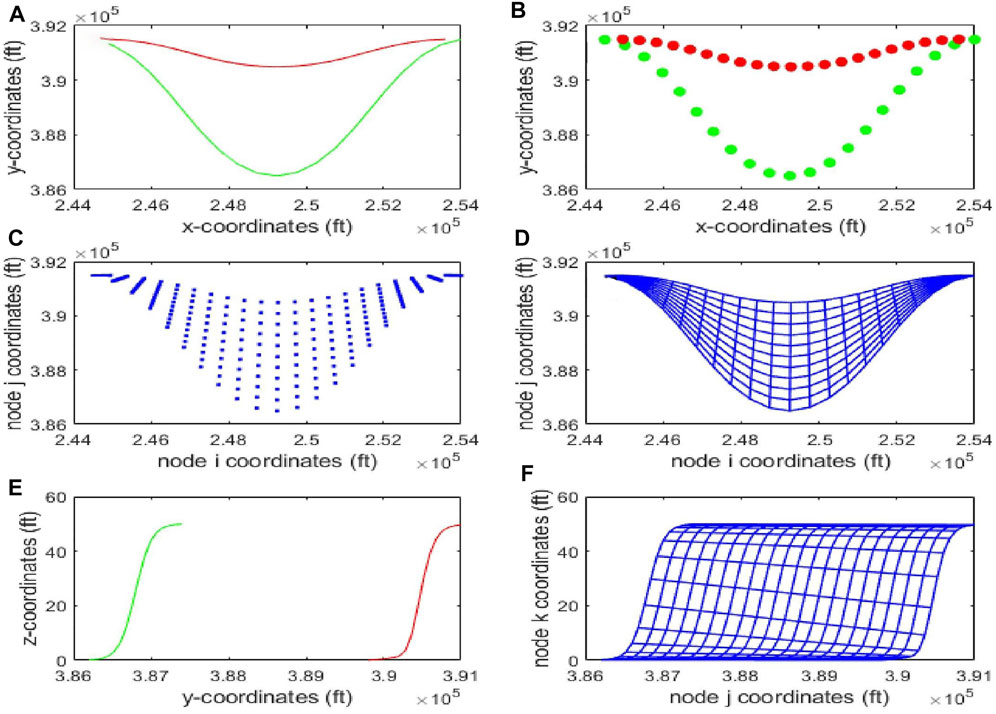
FIGURE 5. Grid generation process: (A) domain to be gridded for the lateral accretions, bounded by the initial channel path (red) and current channel path(green), (B) grid nodes computed along each channel meander path, (C) grid nodes computed between the channel meanders, to complete the gridding of lateral accretions, (D) equivalent curvilinear grid and (F) equivalent curvilinear grid for the IHS. (E) IHS domain to be gridded, bounded by the reservoir top (green) and bottom IHS surfaces(red).

The same procedure is repeated to generate the grid for the IHS (see Figures 5E,F).

Combining the grids for the IHS and the lateral accretions generates a 3D grid for the entire point bar.

$x_{ij}=X_{ij}\pm \left(j-1\right)\cdot \frac{D_{ij}}{ny}\cdot \cos {\alpha }_{ij}(\mathrm{3a})$

$y_{ij}=Y_{ij}\pm \left(j-1\right)\cdot \frac{D_{ij}}{ny}\cdot \sin {\alpha }_{ij}(\mathrm{3b})$

where $D_{ij} \text{and} {\alpha }_{ij}$ are respectively, the distance and angle between a grid node at position $i,j$ on the current meander path and its pair on initial meander path; $ny$ is number of grid blocks between meanders; $X_{ij}$ and $Y_{ij}$ are grid node coordinates along meanders.

2.1.5 Geostatistical Simulation on a Transformed Grid

As indicated earlier, traditional geostatistical methods when applied on regular Cartesian gids cannot properly preserve the curvilinear characteristics and the heterogeneity of point bars. To overcome this challenge, a grid transformation scheme was incorporated. Grid transformation is a way of standardizing the position parameters with respect to the channel boundaries, where the layers are unraveled and flattened onto an orthogonal grid. Geostatistical simulation is then conducted in the transformed space, after which the properties are mapped back into the original curvilinear grid. A summary of this workflow is shown in Figure 6. To account for the pinch out of point bars, the pinch-out grid blocks are treated as net-effective zero thickness blocks, using volume modifiers; therefore, the pinch-out arrays will not contribute to fluid flow to affect flow simulation results.

FIGURE 6

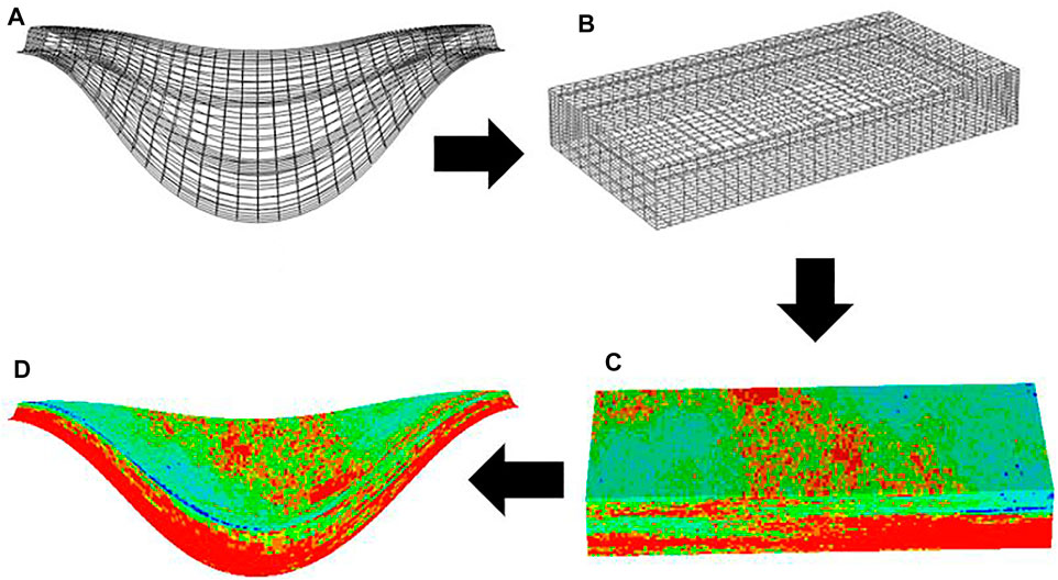
FIGURE 6. Outline of property modeling: (A) point bar curvilinear Grid (B) Orthogonal grid transformation (C) Geostatistical simulation on transformed grid (D) back transformation, indicating the 3D distribution of reservoir properties in the final point bar model.

Identifying the direction of spatial continuity is also necessary for preserving the heterogeneities and depositional trends. For point bars, maximum continuity is in the downstream direction while least continuity is in the perpendicular direction between successive IHS sets (i.e., accretion direction). Between these limits is the medium continuity, which occurs in the dip direction. Accordingly, the maximum range $\left(h_{max}\right)$, medium range $\left(h_{med}\right)$ and minimum range $\left(h_{min}\right)$ were chosen to be in the direction of continuity in the downstream flow, dip, and accretion directions, respectively. Figure 7 shows the directions of spatial continuity as depicted in curvilinear and orthogonal space. The point bar is modeled with 5 inclined layers (i.e., IHS sets) and for each set, $h_{max}$, $h_{med}$ and $h_{min}$ were specified as the major, medium, and minor axis of anisotropy, respectively, for the variogram model (Table 1). Using the SGSIM algorithm (Deutsch & Journel, 1998; Remy, 2004), the IHS sets were modeled separately on an orthogonal grid with dimensions $150\times 30\times 25$. The complete 3D point bar model was obtained by stacking the IHS sets orderly from set 1 to 5 and mapping their properties into the point bar curvilinear grid of dimensions $150\times 150\times 25$ (see Figure 8A). Typical trends seen in point bar systems like the Cranfield reservoir include overall fining up trend in the sediments. High porosity sediments like conglomerates occupy the bottom of the sequence followed by relatively lower porosity sediments like sandstones, muddy-sandstones, and mudstones. These trends were imposed in the simulation with locally varying prior probabilities. It was ensured that the probability of encountering high porosity is maximum at the bottom of each IHs set and minimum at the top. Horizontal slices taken at different depths across the point bar illustrate a fining upward trend as captured in the geostatistical simulation (see Figures 8B–D).

FIGURE 7

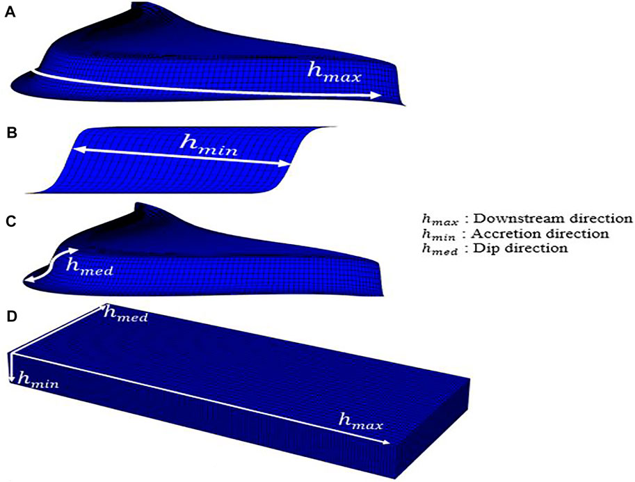
FIGURE 7. Variogram directions in (A,B,C) curvilinear grid and (D) rectilinear grid. h_max, h_med and h_min are in the downstream direction, dip direction and accretion direction, respectively. Please note: the lengths of arrows indicated here are not depicting the magnitude of the ranges; they are just guiding the reader in identifying the directions of spatial continuities.

TABLE 1

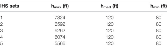
TABLE 1. Variogram inputs for SGSIM.

FIGURE 8

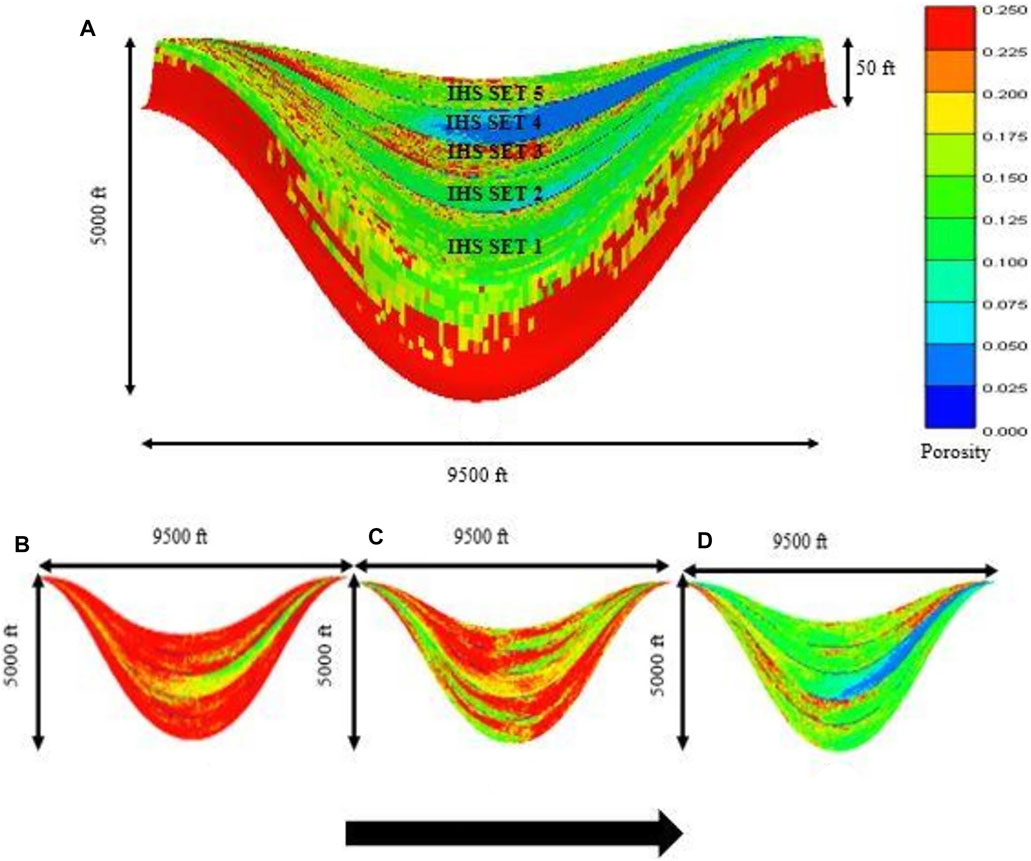
FIGURE 8. (A) single SGSIM realization of property distribution for the various IHS sets within the point bar. Downstream direction is from left to right. (B) Horizontal slices taken at the bottom, (C) mid-section and (D) top of the point bar, showing fining upward trend. Arrow points to the top of the point bar.

The point bar property model displayed here is one of the $50$ realizations that were generated using geostatistical simulation. The reservoir response computed over the suite of realizations would provide an assessment of uncertainty associated with response predictions. For a reliable assessment of the CO₂ sequestration potential of the point bar reservoir, the uncertainty in the point bar geologic model must be reduced by constraining the model to available flow-related data. In the next section, we will discuss how to achieve this by further conditioning the realizations of the point bar model to observed CO₂ injection data.

2.2 Point Bar Reservoir Model Calibration

Model calibration (history matching) is an essential step in characterizing reservoirs and forecasting future reservoir performance. It is grounded on the premise that the static or primary reservoir variables (e.g., porosity, permeability, seismic behavior etc.), influence the dynamic or secondary response of the reservoir (e.g., bottom-hole pressure, CO₂ saturation, CO₂ injectivity etc.). Accordingly, in this study, the static reservoir variables will be systematically adjusted to ensure that simulated dynamic variables acceptably agree with the observed historic data.

In the model calibration procedure, we consider the fact that: 1) reservoir geometry influences fluid flow response variables (e.g., pressure and transmissibility), and therefore should be accounted for in the history matching, 2) the Cranfield reservoir exhibits non-gaussian characteristics (due to the continuity of the depositional structure); and furthermore, the joint relationship between the primary reservoir variable (like permeability), and the secondary variable (like bottom-hole pressure) is non-linear. We use a two-step ensemble-based data assimilation procedure where: step 1 uses ensemble Kalman filter (EnkF) to update ensembles of point bar reservoir model geometries, to select the geometry that yields the closest match to observed data; and step 2 applies indicator-based data assimilation (InDA) to update ensembles of permeability models within the optimal reservoir geometry determined in step1.

2.2.1 Point Bar Geometry Calibration

With the limited coverage of wells in the CO₂ injection area, there is likely to be significant uncertainty associated with the prediction of reservoir geometry. Calibrating models for point bar geometry using injection data is necessary to constrain the uncertainty. Every angular displacement ($\omega$) in the SGF defines a unique point bar geometry; therefore, 50 realizations of $\omega$ were drawn from a normal distribution with mean 35 and standard deviation 10, to generate an ensemble of point bar reservoir geometries. Figure 9 shows some of the realizations of point bar geometry ensembles that were generated. The ensemble of geometries are the initial uncertainties that would be updated upon the availability of secondary variables (e.g., bottom-hole pressure, reservoir pressure, injection rate). Using CMG-GEM simulator (CMG-GEM, 2019), flow simulation was run on the ensemble for a period of $450$ days. The geometries were described using curvilinear grids of dimension $150\times 150\times 25$, making $562500$ grid blocks in total. Reservoir properties like porosity and permeability were kept the same over the ensemble. The injection schedule used for simulation is shown in Figure 10.

FIGURE 9

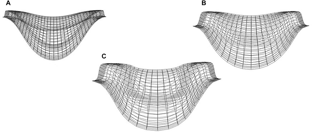
FIGURE 9. Randomly selected realizations of the point-bar reservoir geometries used for performing EnKF. Perturbation of the angular displacements of the sine generation function used to represent the lateral migration of the points bars at (A) ω = 19.4° (B) ω = 45° and (C) ω = 36°. In the EnKF, only the geometry was altered, reservoir properties like porosity and permeability were not changed. The figure is displayed in the Computer Modeling Group (CMG) Software.

FIGURE 10

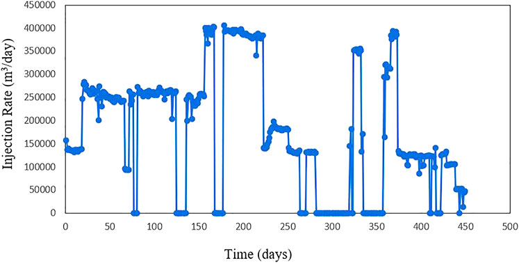
FIGURE 10. Cranfield CO₂ injection schedule used for simulation at injection well F1.

Flow simulation was conducted on the ensemble to obtain the corresponding simulated dynamic bottom-hole pressures that can be used to infer the required covariance between state parameters, and subsequently update the initial geometry ensembles. The error variance representing the measurement error is made proportional to the variance of bottom-hole pressure observed over the ensemble. Updates were performed on the reservoir geometries using the EnKF formulation in Eq. 4 (Kumar and Srinivasan, 2019).

$z_o^a= z_o^f+{\left[C_{pz}\left(h_{jo}\right)\right]}_{1\times n}{\left[{\left[C_p\left(h_{lj}\right)\right]}_{n\times n}+diag{\left[C_{\in \in }\left(h_{lj}\right)\right]}_{n\times n}\right]}^{-1}{\left[P_{obs}-P_{sim}\right]}_{n\times 1}(4)$

In Equation 4, $C_{pz}\left(h_{jo}\right)$ terms are the covariance between the primary and secondary variables, the matrix containing the $C_p\left(h_{ij}\right)$ terms are the covariance between the dynamic response variables. Equation 4 yields the updates $z_o$ for the ensemble locations $o=\mathrm{1,2,3...}n$; $z_o^f$ is the initial value of the primary variable, which is angular displacement in our case; The superscript $a$ represents the updated value. $P_{obs}$ and $P_{sim}$ are respectively, the observed and simulated secondary variables, which are bottom-hole pressures in our case. $\in$ is a vector of uncorrelated observation errors (which is made proportional to the variance of pressures observed over the ensemble), $C_{\in \in }$ therefore becomes a diagonal matrix. To account for possible errors in the observations, samples (number of samples equals the size of ensemble being used) drawn from the distribution $N(0,C_{\in \in })$ are added to the observed data. (Please note that in this study $C_{\in \in }=10 kPa$).

The update (or error) term constitutes all the terms after the first term in Eq. 4. Figure 11B illustrates the updates realized after EnKF implementation. It could be observed that the updates at higher angles are higher than those at lower angles. After performing EnKF updates and running flow simulation on the updated ensembles, a reduction in the spread (i.e., uncertainty) in the simulated bottom-hole pressures is observed (see Figures 11A,C). The reservoir geometry with the least uncertainty (i.e., least error) has an approximate angular displacement of $19.4°$. For this reservoir geometry, the update made to the point bar geometry is illustrated as the black point in Figure 11B. The smaller update indicates that the updates using the CO₂ injection data have stabilized. The corresponding simulated bottom-hole pressure after EnKF updates is the red plot in Figure 11C, and the updated geometry is shown in Figure 11D. This reservoir geometry was selected for the next phase of the history matching process.

FIGURE 11

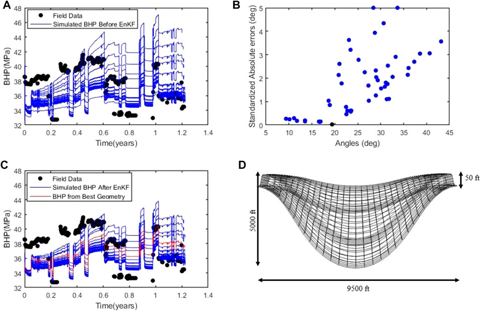
FIGURE 11. Results obtained by applying the EnFK procedure at the end of the simulation period, (A) BHP before EnFK. (B) the updates to the angular displacement obtained using EnFK for various members of the initial ensemble (C) BHP after EnFK. Red plot indicates BHP from geometry with least error (D) Updated point bar geometry with the least error to be used in the next phase of workflow.

Figure 11 also suggests that the geometry alone does not fully explain the dynamic response characteristics of the point bar reservoir under study. A further confirmation is seen after running flow simulation on the ENKF-updated reservoir geometry ensembles. As shown in Figure 11C, after ENKF updates, the simulated bottom-hole pressures still exhibit appreciable uncertainty even though, overall, the uncertainty is reduced. Yet, this calibration step is important as it allows us to select a reservoir geometry that will ensure a more successful history match of static reservoir properties.

Please note that the standardized errors on Figure 11B, denoted $SE\in \left[a,b\right]$ were obtained by using Eq. 5, to scale the updates to a desired range $\left[a,b\right]$.

$SE=\frac{E-\text{min}\left(E\right)}{\max \left(E\right)-\text{min}\left(E\right)}\cdot \left(b-a\right)+a(5)$

where $E$ is the absolute error or update and $SE$ is the standardized absolute error for the ensembles.

2.2.2 Indicator-Based Data Assimilation

In indicator-based method, reservoir properties like permeability are transformed into binary indicator variables of 1s and 0s. Updates are performed by updating the conditional cumulative distribution function $\left(ccdf\right)$ of the variable. There is no assumption made regarding the form of the $ccdf$. Therefore, InDA is free from the Gaussian assumptions that underly ensemble Kalman filter. Before applying InDA to update the geologic models, a brief description of InDA is presented below.

Definition of Indicator Thresholds

In indicator transformation, thresholds $\left(z_k\right)$ are applied to define the binary variables. The thresholds are quantiles (samples) retrieved to adequately capture the distribution $\left(cdf\right)$ of the variable. Therefore, relatively more quantiles are retrieved from portions of the $cdf$ that correspond to major variations in permeability values.

Indicator Definition of the Primary Variable

The defined indicator thresholds form the basis for the indicator definition of the primary variable, so that the indicator definition of a primary variable $Z$, at location $\mathit{u}$ after applying $K$ thresholds, $z_1,z_2\dots z_k$ , can be defined over the entire $n$ ensemble of models as:

$I\left(Z{}_{\text{α}}{}^f\left(\mathit{u}\right),z_k\right)=\{\begin{array}{c}1if Z_{\text{α}}^f\le z_k\\ .\\ 0if Z_{\text{α}}^f>z_k\end{array}k=\mathrm{1,2,3}\dots K(6)$

where $Z_{\text{α}}^f$ is the value before update for an ensemble member α; $\text{α}=\mathrm{1,2,3}\dots n$

Indicator Definition of the Secondary Variable

The secondary variables are dynamic because they change with time as the flow simulation runs. Therefore, instead of applying the threshold definitions on the secondary variable itself, we apply the indicator definition on the mismatch $\left(\left|\Delta P\right|\right)$ between the observed $\left(P_{ob{s}_{\alpha }}^f\right)$ and simulated $\left(P_{si{m}_{\alpha }}^f\right)$ secondary variables. The mismatch can be defined as:

$\left|\mathrm{\Delta }P\right| = \left|P_{ob{s}_{\alpha }}^f-P_{si{m}_{\alpha }}^f\right|(7)$

The indicator definition applied on $\left|\mathrm{\Delta }P\right|$ at a given threshold $|\mathrm{\Delta }P{|}_p$, denoted $Y_p$ can then be expressed as:

$Y_p =Y_p\left(\left|\mathrm{\Delta }{P}_{\alpha }^f\right|,{\left|\mathrm{\Delta }P\right|}_p\right) = \{\begin{array}{c}1\forall \left|\mathrm{\Delta }{P}_{\alpha }^f\right|\le |\mathrm{\Delta }P{|}_p\\ 0\text{otherwise}\end{array}p=\mathrm{1,2,3}\dots n(8)$

In defining thresholds based on data mismatch, the key idea is to choose the thresholds such that the updated conditional cdf of the static variable (for our case, permeability) does not change significantly when the threshold for the data mismatch is perturbed around the optimum. For details about the criterion for selection of secondary thresholds and the theory behind the InDA formulation, the reader is referred to (Kumar and Srinivasan, 2019).

Updating the Static Variable Using InDA Procedure

The applied thresholds and indicator definitions are used in the InDA formulation to perform updates. Updates are performed by updating the cumulative density function $\left(cdf\right)$ of the primary variable. In the InDA formulation, the update $cdf$ equation, expressed as a conditional expectation of the indicator variables is written as:

$F\left(Z_{\alpha }^f(u)\le z_k|Y_p\right)=E\left((I(Z_{\alpha }^f(u),z_k)\right)+{\displaystyle \sum _{i=1}^{i=n}{\lambda }_i}\left(Y_i-E(Y_i)\right)(9)$

Like the EnKF update equations discussed previously, ${\lambda }_i$ are the Kalman gain computed on the basis of the indicator cross-covariance between the primary indicator data I and the secondary indicator data Y. InDA is immune to non-linear transformations because of the binary nature of the indicator variable. In addition, it does not suffer from Gaussian assumptions as applying Eq. 9 directly generates the conditional $cdf$ without making any parametric assumptions.

Using the point bar geometry corresponding to the lowest error, the next task is to perturb the spatial variation of rock properties to match the observed data. Like the traditional geostatistical methods, InDA runs optimally on orthogonal grids; therefore, we modified its implementation by incorporating the grid transformation scheme within the update process.

2.2.3 Implementing InDA to Update the Point bar Model

Indicator-based data assimilation was used to update ensembles of permeability models for the point bar reservoir as follows:

Generation of Initial Ensembles and Reference Model

At the time of modeling, hard data for permeability was not available, therefore, from the porosity ($\varnothing$) ensemble of models that have been generated earlier, the permeability $\left(k\right)$ ensemble of models were generated from Eq. 10, which comes from micro-modeling for enhanced small scale porosity-permeability relationship (Boisvert et al., 2012).

$\ln \left(k\right)=4121.2\cdot {\varnothing }^4+3963.6\cdot {\varnothing }^3-1353.3\cdot {\varnothing }^2+202.05\cdot \varnothing -4.3571(10)$

Defining Primary and Secondary Indicator Thresholds

The use of Eq. 9 for performing updates is contingent upon defining appropriate indicator thresholds for the primary and secondary variables. Figure 12A represents the $cdf$ of the reference permeability model under consideration, and the thresholds that were retrieved. The secondary data thresholds were defined based on the mismatch between the simulated and observed bottom-hole pressure data from the Cranfield injection well (see Figure 12B)

FIGURE 12

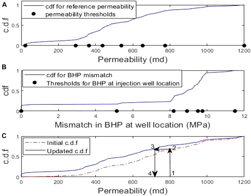
FIGURE 12. (A) cumulative disribution function for permeability for reference model, and the primary indicator thresholds retrieved for permeability distribution, (B) Indicator definitions for Bottom -hole pressure (BHP) at injection well location, and (C) update of primary variable (permeability).

Updating Permeability Using InDA

Using the defined thresholds and the indicator definitions, CO₂ flow simulation was run on the entire initial ensemble of permeability models. Updates were performed by assimilating the mismatch between the observed and simulated bottom-hole pressure at the CO₂ injection well location, using Eq. 9. Figure 12C shows the initial and InDA updated $cdf$ at each location.

To determine the updated permeability whose initial value is say, 800 md, it is read on the horizontal axis (position 1) and the equivalent probability is read on the initial $cdf$ (position 2). This same probability is read on the updated $cdf$ (position 3). The updated permeability value is therefore the permeability that corresponds to the initial probability drawn from the updated $cdf$, which is position 4 on Figure 12C.

3 Results and Discussion

The CO₂ flow simulation was re-run on the updated permeability models to assess the extent to which the simulated bottom-hole pressure matches the observed bottom-hole pressure. We observed an improvement in the match of the updated simulated BHP ensembles to the field BHP data. Comparing the results in Figures 13A,B, it is evident that the uncertainty associated with the prediction of BHP is reduced and the uncertainty distribution better brackets the true response. Additionally, as can be observed in the mean BHP trends (Figures 13C,D), even though the historic data (field data) is not exactly reproduced, the update procedure brings the response of the models closer to the true response. The closer match of the updated models to the field data (true response) can be attributed to the more accurate spatial distribution of permeability obtained by applying the history matching process. The simulation was then run in a forecast mode for the next $50$ years, and the uncertainty evolution of the CO₂ plume was analyzed. Figure 14 shows the uncertainty in the various responses before and after ensemble permeability updates. As observed in this figure, there is a reduction in the variance associated with the predictions and therefore, with the uncertainty in the prediction of the CO₂ displacement after performing updates. The trapped CO₂ (also called residual trapped CO₂) saw the most significant reduction in uncertainty as illustrated in Figures 14A,B. The reduction in uncertainty is most likely due to more accurate representation of the reservoir architecture and spatial distribution of reservoir permeability after performing updates.

FIGURE 13

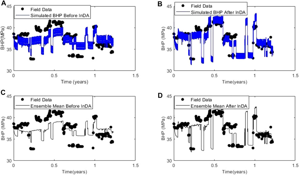
FIGURE 13. History Matching Results. (A) simulated bottom-hole pressure before InDA, (B) simulated bottom-hole pressure after InDA, (C) Ensemble mean before InDA, and (D) Ensemble mean after InDA.

FIGURE 14

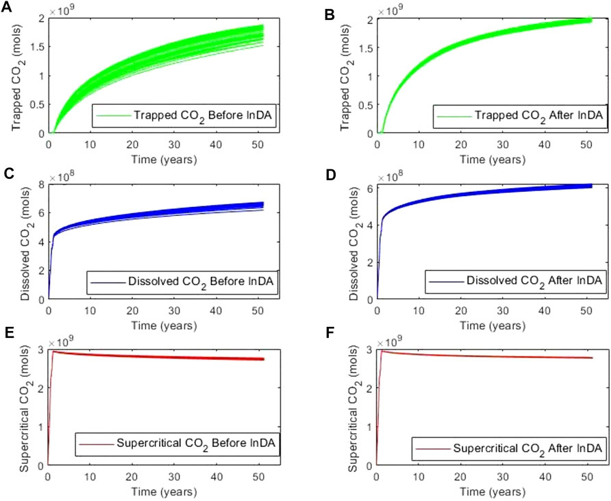
FIGURE 14. CO₂ sequestration responses before and after permeability updates. Moles of residual trapped gas (A) before InDA and (B) after InDA. Moles of dissolved gas (C) before InDA and (D) after InDA. Moles of super critical CO2 (E) before InDA and (F) after InDA.

Unlike residual trapped CO₂, pressure and temperature drive dissolved CO₂ (Duan and Sun, 2003; Portier and Rochelle, 2005) and supercritical CO₂ (Sapkale et al., 2010). Because the temperature is held constant and pressure is a diffused response, the updating process would not significantly reduce their uncertainty as much as it does to the volume of residual trapped CO₂.

4 Concluding Remarks

A geologic modeling approach that honors the point bar curvilinear geometry and heterogeneities has been presented. The reservoir architecture modeling method uses geometric functions to model the point bar heterogeneities. The spatial modeling of point bar properties is difficult due to its complex geometry, but this was overcome by developing a gridding scheme which accounts for the aerial shape of the accretion surfaces as well as sigmoidal shape of the inclined heterolithic stratifications. A grid transformation scheme was also implemented to allow for optimal geostatistical simulation of the point bar properties.

To ensure reliable assessment and prediction of the CO₂ sequestration potential of the reservoir, the point bar model was calibrated, using a two-step ensemble-based history matching procedure. The history matching accounts for the uncertainty in the point bar geometry, and the non-Gaussian distribution of the point bar permeability. The study used data from the Cranfield, Mississippi CO₂ injection reservoir to assess the uncertainty in CO₂ sequestration potential in the long-term, after updating permeability. Incorporating model calibration after geological modeling offers a reliable way to correctly evaluate the long-term CO₂ sequestration potential in point bar reservoirs.

While the proposed method has the efficacy to perform updates for successful evaluation of reservoir performance, we acknowledge some potential non-uniqueness of the solution in the proposed study. For example, the optimized point bar geometry can change when the permeability and porosity used in the geometry calibration changes. Sequentially updating the geometry and the spatial distribution of porosity and permeability, such that at convergence, we have stable updates of both the geometry and reservoir properties, will be explored in future research to address the possible non-uniqueness of the proposed method.

Additionally, the Cranfield dataset used as conditioning data for the geologic modeling, and subsequent data assimilation were limited. This would impact the extent to which the calibrated models are able to reflect the reservoir flow behavior. Therefore, the results could be improved upon the availability of more conditioning data.

Data Availability Statement

The raw data supporting the conclusion of this article will be made available by the authors, upon reasonable request.

Author Contributions

ID: Conceptualization, Methodology, Investigation, Formal Analysis, Visualization, Software, Data Curation, Writing-Original draft preparation. SS: Conceptualization, Supervision, Writing-Reviewing and Editing, Funding Acquisition, Resources.

Conflict of Interest

The authors declare that the research was conducted in the absence of any commercial or financial relationships that could be construed as a potential conflict of interest.

Publisher’s Note

All claims expressed in this article are solely those of the authors and do not necessarily represent those of their affiliated organizations, or those of the publisher, the editors, and the reviewers. Any product that may be evaluated in this article, or any claim that may be made by its manufacturer, is not guaranteed or endorsed by the publisher.

References

Allen, J. R. L. (1965). A Review of the Origin and Characteristics of Recent Alluvial Sediments. Sedimentology 5, 89–191. doi:10.1111/j.1365-3091.1965.tb01561.x

CrossRef Full Text | Google Scholar

Allen, J. R. L. (1964). Studies in Fluviatile Sedimentation: Six Cyclothems from the Lower Old Red sandstone, Anglowelsh basin. Sedimentology 3 (3), 163–198. doi:10.1111/j.1365-3091.1964.tb00459.x

CrossRef Full Text | Google Scholar

Allen, J. R. (1970). Studies in Fluviatile Sedimentation: a Comparison of Fining-Upwards Cyclothems, with Special Reference to Coarse-Member Composition and Interpretation. J. Sediment. Res. 40, 298–323. doi:10.1306/74d71f32-2b21-11d7-8648000102c1865d

CrossRef Full Text | Google Scholar

Austin-Adigio, M. E., Wang, J., Alvarez, J. M., and Gates, I. D. (2018). Novel Insights on the Impact of Top Water on Steam-Assisted Gravity Drainage in a point Bar Reservoir. Int. J. Energ. Res 42 (2), 616–632. doi:10.1002/er.3844

CrossRef Full Text | Google Scholar

Boisvert, J. B., Manchuk, J. G., Neufeld, C., Niven, E. B., Deutsch, C. V., Boisvert, J. B. Manchuk., et al. (2012). “C. V,” in Micro-modeling for Enhanced Small Scale Porosity-Permeability Relationships. Editors P. Abrahamsen, R. Hauge, and O. Kolbjørnsen (Dordrecht: Springer).Geostatistics Oslo

Google Scholar

Boisvert, Jeffery. B. (2011). Conditioning Object Based Models with Gradient Based Optimization. Available at: http://www.ccgalberta.com.20111

Google Scholar

Caers, J., and Zhang, T. (2005). Multiple-point Geostatistics: A Quantitative Vehicle for Integrating Geologic Analogs into Multiple Reservoir Models. AAPG Memoir 80, 383–394.

Google Scholar

CMG-GEM (20192019). Compositional and Unconventional Simulator. Version 2019.10 User’s Guide, 10. Calgary, Alberta: Computer Modeling Group Ltd.

Google Scholar

Daley, T. M., Hendrickson, J., and Queen, J. H. (2014). Monitoring CO2 Storage at Cranfield, mississippi with Time-Lapse Offset VSP - Using Integration and Modeling to Reduce Uncertainty. Energ. Proced. 63, 4240–4248. doi:10.1016/j.egypro.2014.11.459

CrossRef Full Text | Google Scholar

Davies, B. J., and Haldorsen, H. H. (1987). Pseudofunctions in Formations Containing Discontinuous Shales: A Numerical Study. Soc. Pet. Eng. AIME, (Paper) SPE, 221–229. doi:10.2118/16012-ms

CrossRef Full Text | Google Scholar

Delshad, M., Kong, X., Tavakoli, R., Hosseini, S. A., and Wheeler, M. F. (2013). Modeling and Simulation of Carbon Sequestration at Cranfield Incorporating New Physical Models. Int. J. Greenhouse Gas Control. 18, 463–473. doi:10.1016/j.ijggc.2013.03.019

CrossRef Full Text | Google Scholar

Deschamps, R., Guy, N., Preux, C., and Lerat, O. (2011). SPE 147035 Impact of Upscaling on 3-D Modelling of SAGD in a Meander Belt. November.

Google Scholar

Deutsch, Clayton. V., and Journel, A. G. (1998). GSLIB: Geostatistical Software Library. 2nd ed. New York: Oxford University Press.

Google Scholar

Deutsch, C. V. (2006). A Sequential Indicator Simulation Program for Categorical Variables with point and Block Data: BlockSIS. Comput. Geosciences 32 (10), 1669–1681. doi:10.1016/j.cageo.2006.03.005

CrossRef Full Text | Google Scholar

Deutsch, C. V., and Tran, T. T. (2002). FLUVSIM: a Program for Object-Based Stochastic Modeling of Fluvial Depositional Systems. Comput. Geosciences 28, 525–535. doi:10.1016/s0098-3004(01)00075-9

CrossRef Full Text | Google Scholar

Deutsch, C. V., and Wang, L. (1996). Hierarchical Object-Based Stochastic Modeling of Fluvial Reservoirs. Math. Geol. 28 (7), 857–880. doi:10.1007/BF02066005

CrossRef Full Text | Google Scholar

Deveugle, P. E. K., Jackson, M. D., Hampson, G. J., Farrell, M. E., Sprague, A. R., Stewart, J., et al. (2011). Characterization of Stratigraphic Architecture and its Impact on Fluid Flow in a Fluvial-Dominated Deltaic Reservoir Analog: Upper Cretaceous Ferron Sandstone Member, Utah. Bulletin 95, 693–727. doi:10.1306/09271010025

CrossRef Full Text | Google Scholar

Duan, Z., and Sun, R. (2003). An Improved Model Calculating CO2solubility in Pure Waterand Aqueous NaCl Solutions from 273 to 533 K Andfrom 0 to 2000 Bar. Chem. Geology. 193 (3–4), 257–271. doi:10.1016/s0009-2541(02)00263-2

CrossRef Full Text | Google Scholar

Durkin, P. R., Boyd, R. L., Hubbard, S. M., Shultz, A. W., and Blum, M. D. (2017). Three-Dimensional Reconstruction of Meander-Belt Evolution, Cretaceous Mcmurray Formation, Alberta Foreland Basin, Canada. J. Sediment. Res. 87 (10), 1075–1099. doi:10.2110/jsr.2017.59

CrossRef Full Text | Google Scholar

Eskandari, K., and Srinivasan, S. (20182008). Reservoir Modelling of Complex Geological Systems - A Multiple Point Perspective. Can. Int. Pet. Conf., 59–68. doi:10.2118/2008-176

CrossRef Full Text | Google Scholar

Fustic, M., Hubbard, S. M., Spencer, R., Smith, D. G., Leckie, D. A., Bennett, B., et al. (2012). Recognition of Down-valley Translation in Tidally Influenced Meandering Fluvial Deposits, Athabasca Oil Sands (Cretaceous), Alberta, Canada. Mar. Pet. Geology. 29, 219–232. doi:10.1016/j.marpetgeo.2011.08.004

CrossRef Full Text | Google Scholar

Ghazi, S., and Mountney, N. P. (2009). Facies and Architectural Element Analysis of a Meandering Fluvial Succession: the Permian Warchha sandstone,salt Range, Pakistan. Sediment. Geology. 221 (1-4), 99–126. doi:10.1016/j.sedgeo.2009.08.002

CrossRef Full Text | Google Scholar

Gringarten, E., and Deutsch, C. V. (1999). Methodology for Variogram Interpretation and Modeling for Improved Reservoir Characterization. Proc. - SPE Annu. Tech. Conf. Exhibition, OMEGA, 355–367. doi:10.2523/56654-ms10.2118/56654-ms

CrossRef Full Text | Google Scholar

Hartkamp-Bakker, C. ., and Donselaar, M. (1993). “Permeabilitypatterns in point Bar Deposits: Tertiary Loranca Basin, centralSpain,inS,” in The Geological Mod-Elling of Hydrocarbon Reservoirs and Outcrop Analogs. Editors S. Flint, and I. D. Bryant (Oxford: Interna-Tional Association of Sedimentologists Special Publication), 15, 157–168.

Google Scholar

Hathout, D. (2015). Sine-Generated Curves: Theoretical and Empirical Notes. Apm 05 (11), 689–702. doi:10.4236/apm.2015.511063

CrossRef Full Text | Google Scholar

Hovorka, S. D., Meckel, T. A., and Treviño, R. H. (2013). Monitoring a Large-Volume Injection at Cranfield, Mississippi-Project Design and Recommendations. Int. J. Greenhouse Gas Control. 18 (December), 345–360. doi:10.1016/j.ijggc.2013.03.021

CrossRef Full Text | Google Scholar

Issautier, B., Fillacier, S., Le Gallo, Y., Audigane, P., Chiaberge, C., and Viseur, S. (2013). Modelling of CO2 Injection in Fluvial Sedimentary Heterogeneous Reservoirs to Assess the Impact of Geological Heterogeneities on CO2 Storage Capacity and Performance. Energ. Proced. 37, 5181–5190. doi:10.1016/j.egypro.2013.06.434

CrossRef Full Text | Google Scholar

Issautier, B., Viseur, S., Audigane, P., and le Nindre, Y.-M. (2014). Impacts of Fluvial Reservoir Heterogeneity on Connectivity: Implications in Estimating Geological Storage Capacity for CO2. Int. J. Greenhouse Gas Control. 20, 333–349. doi:10.1016/j.ijggc.2013.11.009

CrossRef Full Text | Google Scholar

Kumar, D., and Srinivasan, S. (2019). Ensemble-Based Assimilation of Nonlinearly Related Dynamic Data in Reservoir Models Exhibiting Non-gaussian Characteristics. Math. Geosci. 51 (1), 75–107. doi:10.1007/s11004-018-9762-x

CrossRef Full Text | Google Scholar

Labrecque, P. A., Jensen, J. L., and Hubbard, S. M. (2011). Cyclicity in Lower Cretaceous point Bar Deposits with Implications for Reservoir Characterization, Athabasca Oil Sands, Alberta, Canada. Sediment. Geology. 242 (1–4), 18–33. doi:10.1016/j.sedgeo.2011.06.011

CrossRef Full Text | Google Scholar

Labrecque, P. A., Jensen, J. L., Hubbard, S. M., and Nielsen, H. (2011). Sedimentology and Stratigraphic Architecture of a point Bar deposit, Lower Cretaceous McMurray Formation, Alberta, Canada. Bull. Can. Pet. Geology. 59, 147–171. doi:10.2113/gscpgbull.59.2.147

CrossRef Full Text | Google Scholar

Langbein, W. B., and Leopold, L. B. (1966). River Meanders - Theory of Minimum Variance. U.S. Geol. Surv. Prof. Paper 422-H, H11–H1515. doi:10.3133/PP422H

CrossRef Full Text | Google Scholar

Li, Henry., and Srinivasan, S. (2015). Modeling Point Bars Using a Grid Transformation Scheme Heterogeneities in Point Bars. SPE Annu. Tech. Conf. Exhibition, September, 28–30.

Google Scholar

Li, H., and White, C. D. (2003). Geostatistical Models for Shales in Distributary Channel point Bars (Ferron Sandstone, Utah): from Ground-Penetrating Radar Data to Three-Dimensional Flow Modeling. Bulletin 87, 1851–1868. doi:10.1306/07170302044

CrossRef Full Text | Google Scholar

Lu, J., Kordi, M., Hovorka, S. D., Meckel, T. A., and Christopher, C. A. (2013). Reservoir Characterization and Complications for Trapping Mechanisms at Cranfield CO2 Injection Site. Int. J. Greenhouse Gas Control. 18, 361–374. doi:10.1016/j.ijggc.2012.10.007

CrossRef Full Text | Google Scholar

Miall, A. D. (1988). Architectural Elements and Bounding Surfaces in Fluvial Deposits: Anatomy of the kayenta Formation (Lower Jurassic), Southwest Colorado. Sediment. Geology. 55 (3–4), 233–262. doi:10.1016/0037-0738(88)90133-9

CrossRef Full Text | Google Scholar

Movshovitz-Hadar, N., and Shmukler, A. (2000). River Meandering and a Mathematical Model of This Phenomenon. 25, 123. Available at: http://physicaplus.org.il/zope/home/en/1124811264/1141060775rivers_en.

Google Scholar

Musial, G., Labourdette, R., Franco, J., and Reynaud, J.-Y. (2013). Modeling of a Tide-Influenced Point-bar Heterogeneity Distribution and Impacts on Steam-Assisted Gravity Drainage Production: Example from Steepbank River, McMurray Formation, Canada. AAPG Stud. Geology. 64, 545–564.

Google Scholar

Nardin, T. R., Feldman, H. R., and Carter, B. J. (2013). Stratigraphic Architecture of a Large-Scale point-bar Complex in the McMurray Formation: Syncrude’s Mildred Lake Mine, Alberta, Canada. AAPG Stud. Geology. 64, 273–311. doi:10.1306/13371583st643555

CrossRef Full Text | Google Scholar

Nazeer, A., Abbasi, S. A., and Solangi, S. H. (2016). Sedimentary Facies Interpretation of Gamma Ray (GR) Log as Basic Well Logs in Central and Lower Indus Basin of Pakistan. Geodesy and Geodynamics 7 (6), 432–443. doi:10.1016/j.geog.2016.06.006

CrossRef Full Text | Google Scholar

Niu, B., Bao, Z., Yu, D., Zhang, C., Long, M., Su, J., et al. (2021). Hierarchical Modeling Method Based on Multilevel Architecture Surface Restriction and its Application in point-bar Internal Architecture of a Complex Meandering River. J. Pet. Sci. Eng. 205 (April), 108808. doi:10.1016/j.petrol.2021.108808

CrossRef Full Text | Google Scholar

Odundun, O., and Nton, M. (2011). Facies Interpretation from Well Logs: Applied to SMEKS Field, Offshore Western Niger Delta, 25. American Association of Petroleum Geologists.

Google Scholar

Olulana, O. O. (2015). Stochastic Modeling of Channel Meanders and Resultant Point Bars.

Google Scholar

Portier, S., and Rochelle, C. (2005). Modelling CO2 Solubility in Pure Water and NaCl-type Waters from 0 to 300 C and from 1 to 300 Bar: Application to the Utsira Formation at Sleipner. Chem. Geology. 217 (3–4), 187–199. doi:10.1016/j.chemgeo.2004.12.007

CrossRef Full Text | Google Scholar

Pranter, M. J., Ellison, A. I., Cole, R. D., and Patterson, P. E. (2007). Analysis and Modeling of Intermediate-Scale Reservoir Heterogeneity Based on a Fluvial point-bar Outcrop Analog, Williams Fork Formation, Piceance Basin, Colorado. Bulletin 91 (7), 1025–1051. doi:10.1306/02010706102

CrossRef Full Text | Google Scholar

Pyrcz, Michael. J., and Deutsch, C. V. (2004). “Stochastic Modeling of Inclined Heterolithic Stratification with the Bank Retreat Model,” in Proceedings of the 2004 Canadian Society of Petroleum Geologists, Canadian Well Logging Society and Canadian Heavy Oil Association Joint Convention (ICE 2004) (Calgary, Canada.8

Google Scholar

Pyrcz, Michael. J. (2001). Bank Retreat Meandering Fluvial Process-Based Model. 1–12.

PubMed Abstract | Google Scholar

Pyrcz, M. J., Boisvert, J. B., and Deutsch, C. V. (2009). ALLUVSIM: A Program for Event-Based Stochastic Modeling of Fluvial Depositional Systems. Comput. Geosciences 35, 1671–1685. doi:10.1016/j.cageo.2008.09.012

CrossRef Full Text | Google Scholar

Pyrcz, M. J., Catuneanu, O., and Deutsch, C. V. (2005). Stochastic Surface-Based Modeling of Turbidite Lobes. Bulletin 89 (2), 177–191. doi:10.1306/09220403112

CrossRef Full Text | Google Scholar

Remy, N. (2004). Geostatistical Earth Modeling Software: User’s Manual, 1–87. Available at: papers2://publication/uuid/D72A1F6E-10B2-4C84-864E-7840DE1414BA

Google Scholar

Richardson, J. G., Harris, D. G., Rossen, R. H., and Van Hee, G. (1978). The Effect of Small, Discontinuous Shales on Oil Recovery. J. Pet. Tech. 30, 1531–1537. doi:10.2118/6700-pa

CrossRef Full Text | Google Scholar

Sapkale, G. N., Patil, S. M., Surwase, U. S., and Bhatbhage, P. K. (2010). Supercritical Fluid Extraction. Int. J. Chem. Sci. 8 (2), 729–743.

Google Scholar

Shu, X., Hu, Y., Jin, B., Dong, R., Zhou, H., and Wang, J. (2015). Modeling Method of Point Bar Internal Architecture of Meandering River Reservoir Based on Meander Migration Process Inversion Algorithm and Virtual Geo-Surfaces Automatic Fitting Technology. SPE Annu. Tech. Conf. Exhibition 30. doi:10.2118/175013-MS

CrossRef Full Text | Google Scholar

Stephen, K. D., Clark, J. D., and Gardiner, A. R. (2001). Outcrop-based Stochastic Modelling of Turbidite Amalgamation and its Effects on Hydrocarbon Recovery. Pet. Geosci. 7 (2), 163–172. doi:10.1144/petgeo.7.2.163

CrossRef Full Text | Google Scholar

Su, Y., Wang, J. Y., and Gates, I. D. (2013). SAGD Well Orientation in point Bar Oil Sand deposit Affects Performance. Eng. Geology. 157, 79–92. doi:10.1016/j.enggeo.2013.01.019

CrossRef Full Text | Google Scholar

Sun, Z., Lin, C., Zhu, P., and Chen, J. (2017). Analysis and Modeling of Fluvial-Reservoir Petrophysical Heterogeneity Based on Sealed Coring wells and Their Test Data, Guantao Formation, Shengli Oilfield. J. Pet. Sci. Eng. 162, 785–800. doi:10.1016/j.petrol.2017.11.006

CrossRef Full Text | Google Scholar

Thomas, R. G., Smith, D. G., Wood, J. M., Visser, J., Calverley-Range, E. A., and Koster, E. H. (1987). Inclined Heterolithic Stratification-Terminology, Description, Interpretation and Significance. Sediment. Geology. 53, 123–179. doi:10.1016/s0037-0738(87)80006-4

CrossRef Full Text | Google Scholar

Visher, G. (1964). Fluvial Processes as Interpreted from Ancient and Recent Fluvial Deposits. AAPG Bull. 48, 550. doi:10.1306/bc743d0d-16be-11d7-8645000102c1865d

CrossRef Full Text | Google Scholar

Willis, B. J., and Tang, H. (2010). Three-dimensional Connectivity of point-bar Deposits. J. Sediment. Res. 80 (5–6), 440–454. doi:10.2110/jsr.2010.046

CrossRef Full Text | Google Scholar

Willis, B. J., and White, C. D. (2000). Quantitative Outcrop Data for Flow Simulation. J. Sediment. Res. 70, 788–802. doi:10.1306/2dc40938-0e47-11d7-8643000102c1865d

CrossRef Full Text | Google Scholar

Wilson, B. W., and Nanz, R. H. (1959). “Sand Conditions as Indicated by the Self-Potential Log,” in EPRM Memorandum Report.

Google Scholar

Yang, C., Romanak, K., Hovorka, S., Holt, R. M., Lindner, J., and Trevino, R. (2013). Near-surface Monitoring of Large-Volume CO2 Injection at Cranfield: Early Field Test of SECARB Phase III. SPE J. 18 (3), 486–494. doi:10.2118/163075-PA

CrossRef Full Text | Google Scholar

Yin, Y. (2013). A New Stochastic Modeling of 3-D Mud Drapes inside Point Bar Sands in Meandering River Deposits. Nat. Resour. Res. 22 (4), 311–320. doi:10.1007/s11053-013-9219-3

CrossRef Full Text | Google Scholar

Yue, W., and Shiyue, C. (2016). Meandering River Sand Body Architecture and Heterogeneity: A Case Study of Permian Meandering River Outcrop in Palougou, Baode, Shanxi Province. Pet. Exploration Dev. 43 (2), 230–240.

Google Scholar

Zhang, R., Song, X., Fomel, S., Sen, M. K., and Srinivasan, S. (2013). “Time-lapse Seismic Registration and Inversion for CO 2 Sequestration Study at Cranfield Part II,” in Pre- stack Analysis SEG Houston 2013 Annual Meeting SEG Houston 2013 Annual Meeting, 5015–5020.

Google Scholar