Climatic Impacts of Wind-Wave-Wake Interactions in Offshore Wind Farms

1 Introduction

The installed capacity of offshore wind energy has continuously increased in the past years (Díaz and Guedes Soares, 2020) and is expected to increase in the future (IRENA, 2019). Accuratewind resource assessments are crucial to make these investments cost-effective. Even though modelling the wind field offshore seems simpler than over complex terrain onshore, challenges remain (Veers et al., 2019). In contrast to most sites onshore, the roughness length of the surface offshore is not static, but changes dynamically with sea state (e.g. Drennan, 2003; Du et al., 2017; Porchetta et al., 2019). The local sea state is a complex superposition of different waves: locally generated from the local wind field, or remotely generated swell.

Previous studies, using Large Eddy Simulations (LES), unsteady Reynolds-averaged Navier-Stokes (URANS) as well as mesoscale model simulations, have found an impact of the wave field on the wind field that can reach into heights of the turbine rotor height (Jenkins et al., 2012; Kalvig et al., 2014; Paskyabi et al., 2014; Yang et al., 2014; AlSam et al., 2015; Zou et al., 2018; Wu et al., 2020; Porchetta et al., 2021). The wave impacts can increase and decrease the wind resources. Largest increases were found during aligned wind-wave conditions (Porchetta et al., 2021) and during swell under moderate winds (Kalvig et al., 2014; Yang et al., 2014; AlSam et al., 2015; Lyu et al., 2018). Largest reductions in wind resources due to waves were found during short fetches (Jenkins et al., 2012), which are often associated with wind-wave misalignment (Kalvig et al., 2014; Porchetta et al., 2021), with rapidly changing winds corresponding to young wave age (Jenkins et al., 2012). These studies illustrate that Charnock-based model parameterizations (Edson et al., 2013), which are typically used in standalone uncoupled atmosphere models to derive wind resources, cannot fully capture the complex interaction between waves and winds. However, even more complex parameterizations of wave conditions (Drennan, 2003; Porchetta et al., 2019) still cannot capture all effects, because they only consider a limited set of wave parameters to derive the wave impact on roughness length. The Wave Boundary Layer Model (WBLM) by Du et al. (2017, 2019) aims to fill this gap by calculating the momentum transfer between atmosphere and waves in mesoscale models in a matter that is energy- and flux-consistent.

Offshore wind farms (OWFs) are not passively exposed to the wave-affected wind field. Instead they extract kinetic energy from the atmospheric flow and increase turbulence and thereby actively change the wind resources downstream. Different studies have investigated how the wake recovery differs for different wave states and found that wake-wave interaction also modifies wind resources downstream. Ferčák et al. (2022) used a wind turbine model in a combined wave tank and wind tunnel to study the wake recovery of a single turbine under three wave conditions: wind-driven waves only and wind-driven waves plus waves with generated by a wave paddle with a period of 0.5 and 0.8 s, respectively. They found a dependence of the wake recovery on the wave characteristics and that the wake recovery oscillates, i.e. speeds up and slows down, with the waves. AlSam et al. (2015) used LES simulations to study the recovery of the flow after a single turbine and found longer and narrower wakes during swell, especially swell of higher wave age. While those studies gave insight into the detailed interactions of wind turbines with waves very close to a turbine, they focused on idealized conditions and did not take into account multiple turbines. To fill this gap, Porchetta et al. (2021) conducted realistic mesoscale atmosphere-wave coupled simulations for two periods in the German Bight: one during misaligned wind-wave conditions and one during aligned wind-wave conditions with high significant wave heights. Their results suggest that during periods of aligned wind and waves, power output was higher in the coupled simulation, compared to the uncoupled atmosphere-only simulation. The opposite occurred for misaligned wind and waves. The differences reached as much as 20%. However, they only investigated two short periods. Thus, the question on the importance of coupled simulations for accurate long-term wind resource assessment in the presence of wind farms in the German Bight remains unanswered.

The interaction of wakes and waves also influence the wave field. Bärfuss et al. (2021) analysed airborne laser scanner measurements up- and downwind of a wind farm under fetch-limited conditions in the German Bight and found a redistribution of wave energy from larger to smaller wave length in the wake up to at least 55 km downstream. From a theoretical point of view wind turbines influence waves in two ways: 1) through the interaction with the wind turbine pole due to reflection, diffraction and drag dissipation and 2) though a reduced wind stress as a consequence of the kinetic energy extraction by the turbines (Christensen et al., 2013). Through idealised studies with a uncoupled wave model and an analytical model for wind farm effects on friction velocity, Christensen et al. (2013) found that the effect of drag dissipation is negligible and the influence of the reduced wind stress dominates 2 km downwind of a wind farm for moderate wind speeds of 10 m s⁻¹. The relative small influence of the wind turbine pole on the wave height in the far field of the turbine agrees with the results obtained by Alari and Raudsepp (2012), where they parameterized wind turbines as land in a uncoupled wave model. Ponce de León et al. (2011) used a similar technique and found that the influence of the poles depends on directional distribution of the incoming wave spectrum, but only investigated the wind farm near wake area. Christensen et al. (2013) concluded that considering the trend towards larger and less dense OWFs the influence of reflection and diffraction at the turbines will be reduced, while the influence of the reduced wind stress will remain in the same order of magnitude. Thus, while there is evidence from measurements and idealized simulations that OWFs influence waves, it is likely mostly due to the reduced wind stress, and it remains unclear how strong this effect is in realistic simulations under real-time conditions.

This study will thus address two unconsidered questions, namely 1) How do wind-wave-wake interactions affect long-term offshore wind resources in the German Bight? 2) How do wind-wave-wake interactions affect the long-term waves climatology in the German Bight? To address these questions realistic coupled simulations need to consider all possible wind-wave-wake interactions and be representative of the wind and wave climate in a certain region. To do so, we develop a statistical-dynamical downscaling method and apply it to the offshore area of the German Bight (Section 2.1), which has many newly build wind farms. For the statistically representative days, we perform coupled and uncoupled model simulations using the WBLM to ensure state of the art momentum exchange between atmosphere and waves (Section 2.2). The obtained simulation results are used to address the two research questions in Section 3 and are discussed in Section 4.

2 Methods

2.1 Selection of Representative Days

Different statistical-dynamical downscaling approaches have been proposed to represent long-term wind resources in the literature (Chávez-Arroyo et al., 2018). To reach the goal of the present study, we need to represent both the long-term wind resources and wave climate, and ensure that the relationships between wind and waves are represented accurately. Do to so, we develop a measurement-driven statistical-dynamical downscaling method based on the methods by Boettcher et al. (2015) and Rife et al. (2013).

The basic principle of the selection process is outlined in Figure 1. We select a limited number of dates that combined match the climatic frequency distribution for different variables around the German Bight. To define the climatic frequency distributions, we use measurements around the German Bight from different sources. The measurements are quality-controlled and temporally aligned. Probability density functions for the entire measurement period and randomly sampled days are computed and compared. The final sample days are selected based on the best overall agreement for the distributions of long-term observations and sampled days of several wind and wave variables. The representativeness of the best date combination is checked for joint probability distributions of different variables and the spatial representativeness by comparing it against reanalysis data. By selecting multiple locations, we ensure that the selected days are representative for a larger area.

FIGURE 1

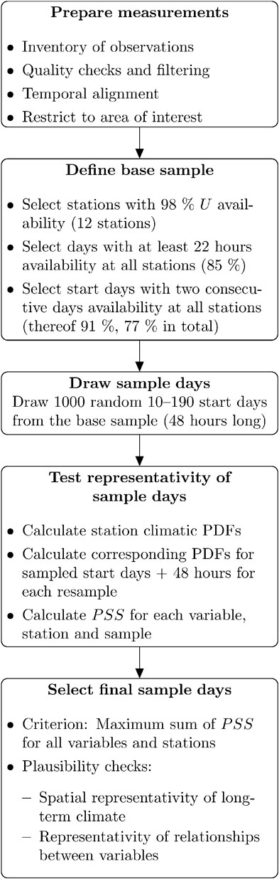
FIGURE 1. Process for selecting statistically representative days of the 30-years wind and wave climate in the German Bight.

2.1.1 Observations and Base Sample

The inventory of observations (Table 1) covers the German Bight and nearby land area (Figure 2). The sites are categorised into atmospheric (“atmos”) sites (measurements of wind speed, U or wind direction, D), “waves” sites (measurements of significant wave height, H_s, peak direction, θ_p or mean wave direction, θ_m) and ‘ocean’ sites (measurements of sea surface temperature, SST, or water temperature, t_w). The data sets differ in the periods covered, their temporal resolutions and averaging times. To align the different measurements time-wise, first the buoy measurements of EMODnet (European Marine Observation and Data network, Emodnet, 2020a) and FINO1 and FINO3 (Forschungsplattformen In Nord- and Ostsee 1 and 3, BSH, 2020) are re-indexed to the nearest full 10 min, secondly the measurements are filtered for suspicious values and thirdly all measurements are hourly averaged to align the temporal frequency of the different data sets. The filtering is done following recommended filter criteria (Supplementary Table S1) for the different data sets (Table 1) and afterwards outliers are detected using the IOOS (Integrated Ocean Observing System) QARTOD (Quality Assurance/Quality Control of Real-Time Oceanographic Data) method (IOOS, 2021). After the automatic checks, a manual visual quality control is performed.

TABLE 1

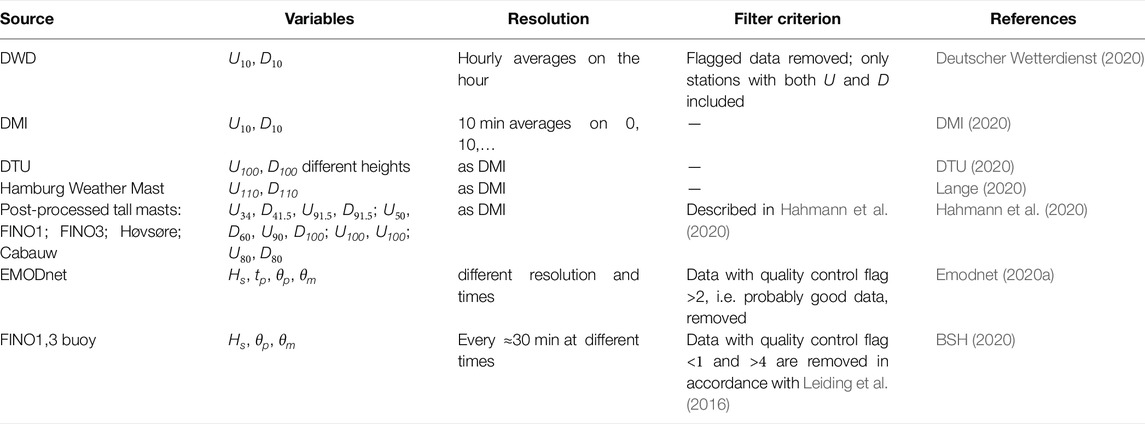
TABLE 1. Details on the observations used in this study.

FIGURE 2

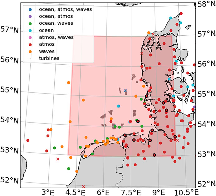
FIGURE 2. Measurements around the German Bight colour-coded based on the observation type. Crosses indicate tall masts. The red area represents the focus area around the existing wind turbines in 2020 (gray dots). Circles with black edges indicate base sample stations.

We created a base sample using the quality controlled data sets, which is used to ensure that sufficient observations are available for the entire period to validate the simulations. Thus, the base sample should have an availability above 98% during the 30 year period. This criterion was only fulfilled by the 10-m wind measurements at the 12 stations around the German Bight (circles with black edge color in Figure 2), which are therefore used as the basis for base sample. The available dates were filtered so that only dates with at least 22 h on each of two consecutive days at all stations are available. A simulation period of two consecutive days is used to balance computational overhead and sufficient meteorological variability between the days. In total 77% of the 30-year period was included in the base sample. The monthly frequency indicates that the availability after the filtering varies slightly throughout the year with lower availability in summer and higher in winter (Supplementary Figure S1). Nevertheless, the minimum summer availability is still about 70% of the 30-year period and the filtering does not introduce a systematic seasonal bias.

2.1.2 Sampling Strategy and Representativity

The base sample (Section 2.1.1) is used to select representative days. For that 10, 20, … , 190 random pairs of two consecutive days N(t) = 20, 40, … 380 are randomly selected from the base sample while ensuring that no date t is selected twice. This random sampling procedure is repeated R = 1000 times to capture the scatter of individual samples.

To derive the representativity of the group of selected days (N(t)), we apply the skill score by Perkins (PSS, Perkins et al., 2007) following the approach in Boettcher et al. (2015). The PSS evaluates how well two discrete PDFs, Z^c(1) and $Z_{N(t)}^s(i)$, overlap for each bin i:

$PSS\left(l,t\right)=\sum _{i=1}^n\min \left(Z^c\left(i,l\right),Z_{N\left(t\right)}^s\left(i,t,l\right)\right).(1)$

Here, Z^c(i, l) is the discrete daily climatic PDF at a certain location l for all hourly measurement times T, i.e. $Z^c(i,l)\equiv Z_T^s(i,l)\equiv Z^s(i,T,l)$. $Z_{N(t)}^s(i,t,l)$ is the daily sample PDF for a certain number of sample days N made up of t days within T. The value of PSS is close to zero for almost no overlap of the two PDFs and approaches one for a perfect match. Since the PSS operates on discrete PDFs, the variables are binned according to Table 2. An example for a climatic PDF Z^c and sample PDFs $Z_{N(t)}^s$ for a collection of dates t is shown in Supplementary Figure S2.

TABLE 2

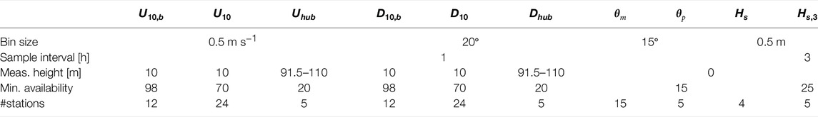
TABLE 2. Bin size, sample interval, measurement height, minimum (min.) availability and number of stations (#stations) for 10-m and hub height (hub) wind speed (U) and wind direction (D) and for the significant wave height (H_s) in one and 3 hour resolution and for wave direction in terms of both peak (θ_p) and mean direction (θ_m). Subscript ‘b’ refers to the base sample (Section 2.1.1).

Figure 3 shows the combined PSS for all base stations (black circles in Figure 2) and all R = 1000 resamples of different collections of dates t for the different sample sizes N in form of boxplots for (A) U and (B) D. Following Perkins et al. (2007) and Boettcher et al. (2015) we classify an agreement between two PDFs as good for PSS > 0.8 (blue line) and as near-perfect for PSS > 0.9 (green line). The red lines indicate the mean and maximum data availability over all stations. Since Figure 3 only shows the results for the base sample, which was selected based on its high data availability (Section 2.1.1, Table 2), the availability is close to 1.

FIGURE 3

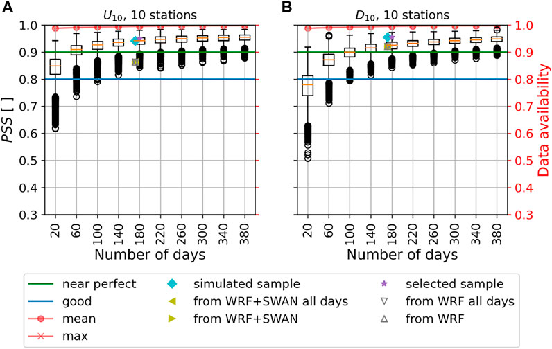
FIGURE 3. Boxplot for the skill score by Perkins PSS for 10-m (A) wind speed U and (B) wind direction D for all resamples for all base sample stations (black circles in Figure 2) along with mean and maximum data availability over all stations. The star indicates the PSS from the selected sample (Section 2.1.3), the diamond the PSS from the simulated sample (Section 2.2) and the triangles the PSS from the simulations (Section 3.1). Note that PSS from all simulations is almost the same and thus all triangles are plotted on top of each other.

The representativity of the group of sampled days for the 12 base sample stations combined (Figure 3) increases with increasing number of sample days. However, depending on the randomly selected sample days, the representativity varies considerably, especially for smaller sample sizes. The spread decreases with increasing sample size and for sample sizes with more than 140 days, all samples provide at least a good representativity at all 12 stations.

The selected sample days should represent the wave climate and hub-height wind climate in accordance with the aim of this study. Thus, a PSS is also derived for all other variables and stations using the bins as in Table 2. Only those stations from Figure 2 are taken into account that cover a minimum period within the 30 years (Table 2). The availability thresholds were chosen to maximize spatial and temporal coverage of the stations and variables, while disregarding stations that are not representative for a long-term climate. The PSS is calculated for those stations using a similar equation as Eq. (1) but now only those randomly selected days that lie within the measurement climate period (m) at that station can be used for comparison. Thus, instead of evaluating the agreement between $Z_{N(t)}^s$ and Z^c, the agreement is evaluated between $Z_{N(t)}^s$ and $Z^{mc}=Z_{Tm}^s$, i.e. including all hourly measurement times T that fall in m. Thus PSS^mc is

${PSS}^{mc}\left(t,l\right)=\sum _{i=1}^n\min \left(Z^{mc}\left(i,l\right),Z_{N\left(t\right)}^s\left(i,t\cap m,l\right)\right)(2)$

As a consequence of using mc, the number of days included in the calculation of PSS^mc varies 1) for each station, as the measurement climate period varies, and 2) for each resample R, as a different number of sample days N(t) can lie within the measurement climate period. Hence, when interpreting the results of PSS^mc one has to keep in mind that even if 180 days are sampled, the number of days included to derive PSS^mc might be smaller. In addition, Z^mc might not fully represent Z^c, since the measurement period covers less than 30 years.

The PSS^mc is shown in Figure 4 for the different variables described in Table 2. The mean and maximum data availability shows the spread of data availability per station and variable. The H_s at 3 hour resolution is used as a separate variable, since those measurements are available for a longer period, as indicated by the higher mean and max availability in Figure 4F compared to Figure 4E.

FIGURE 4

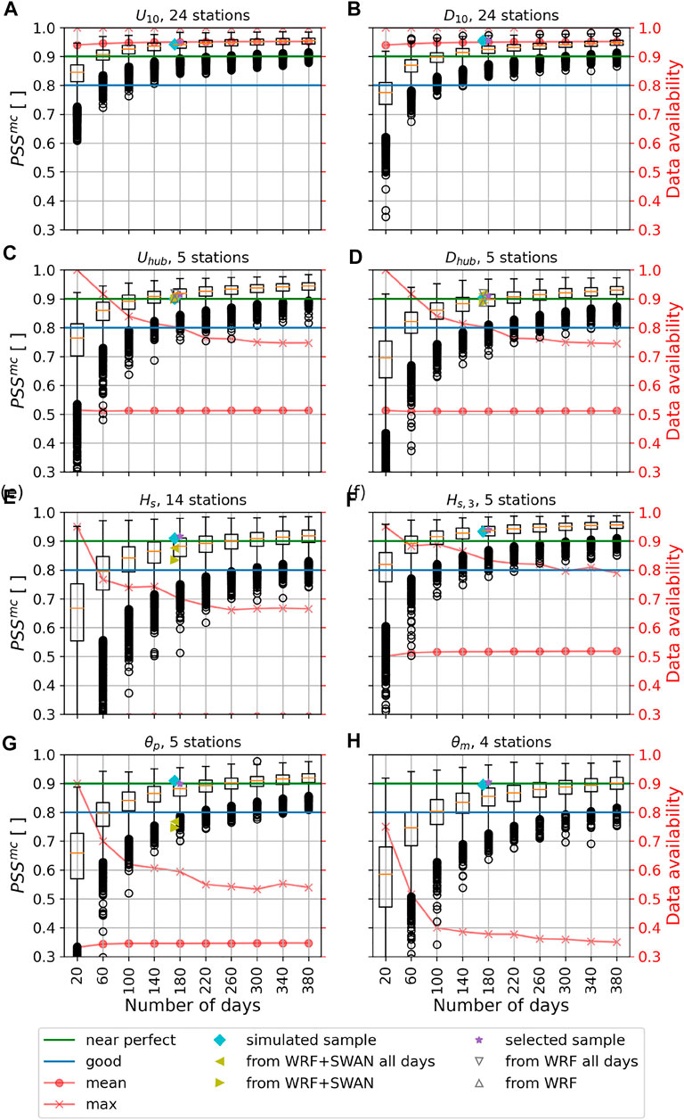
FIGURE 4. Same as Figure 3, but for PSS^mc for (A,B) near surface wind speed and direction (C,D) hub-height wind speed and direction (E,F) significant wave height for one and 3 hour resolution and (G,H) peak and mean wave direction. Mean availability for θ_m is below 0.3 and thus not visible in (h).

Similar to the results for the base sample (Figure 3), PSS^mc increases with increasing number of sample days. However, the number of days required to represent the long-term conditions in a good-to-near-perfect way, differs for each variable. The long term wind climate is better represented close to the surface compared to hub height, especially for D_hub. This is due, among other factors, to the relatively low availability of measurements (50%, red line with dots), which means that in practice only about half of the sample days are used to calculate PSS^mc. However, even for D_hub, the median is close to near perfect for 180 or more samples. This indicates that the surface and hub height wind climate can be well represented using 180 days.

The wave climate is not as well represented as the wind climate, as indicated by the lower median PSS^mc. However, especially the 3-h H_s shows near perfect agreements with increasing number of samples. The low mean availability of the data indicates that on average less than half of the number of days could actually be evaluated. However, even under this constrain the wave climate should be reasonably represented, if actually at least 180 days are used.

In conclusion, using a sample of 180 days can well represent the 30 years 10-m wind climate around the German Bight and the long-term climate of other variables around the German Bight.

2.1.3 Selection of Final Sample Days

While most combinations of 180 sample days provide good or near perfect representativity depending on the different variables, the R = 1000 resamples indicate that there is still a lot of spread. Thus, to find the best possible resample for both wind and wave climate, the maximum sum of the PSS^mc for all variables in Figure 4 for 180 sample days, is used as a criterion. This best overall sample is shown in Figures 3, 4 as a purple star. Supplementary Figure S1 shows that the sample days spread relatively equally over the different months and thus no seasonal bias is evident.

To confirm the representativity of the selected samples, two plausibility checks are performed: Firstly, we use European Centre for Medium-Range Weather Forecasts Reanalysis fifth Generation ERA5 reanalysis data (Hersbach et al., 2018), which can provide a 30 years time series even at stations where the measurement climate is short and provides an opportunity to confirm the spatial pattern of the sampled period. Secondly, we investigate the two-dimensional representativity, i.e. the representativity with respect to variable combinations.

Figure 5A,C show, respectively, the 30-years average wind speed at 100 m and significant wave height based on ERA5 reanalysis. Coloured diamonds show the average U₁₀₀ and H_s at the different measurement stations based on the best 180 sample days. The figures show that the average climate of both hub-height wind speed and significant wave height can be well represented with the sample days and that the spatial pattern around the German Bight is met. Figure 5B,D shows as boxplot for each station the measurement climate (blue), the measurement distribution from the sample days (orange) as well as the station climate based on ERA 5 (green) and based on ERA5 distribution from the sample days (red). The plot confirms that not only the mean climate is well met by the selected days, but also the distributions as a whole, especially within the inner quantiles. Extreme values cannot be captured with this statistical downscaling method, and those are outside the goal of this study. To capture extremes a different downscaling method was developed by Larsén et al. (2019). The spatial distributions are also well matched for other variables as shown in Supplementary Figures S3–S6.

FIGURE 5

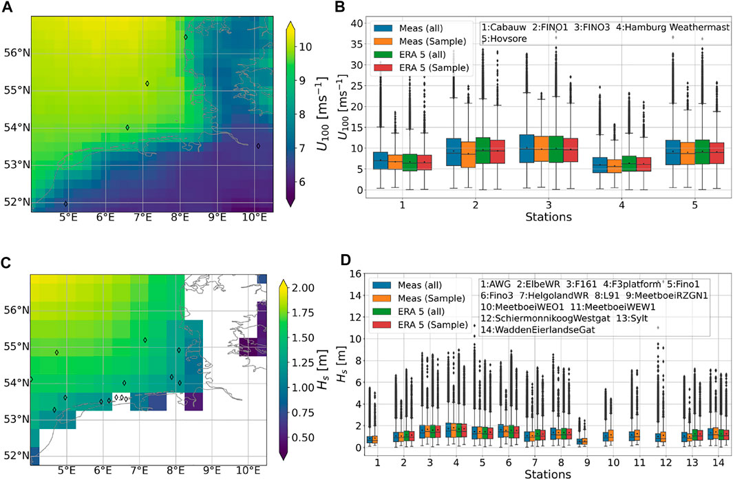
FIGURE 5. ERA5 30-years average (A) wind speed at 100 m height (U₁₀₀) and (C) significant wave height (H_s) with coloured diamonds showing the representativity of the 180 selected days. (B) U₁₀₀ and (D) H_s boxplots of measurement climate (blue) and ERA5 climate (green) per station as well the respective boxplot from the 180 sample days (orange and red, respectively).

So far, the selection of representative days was based on individual variables. However, these variables depend on each other. For instance higher waves in the German Bight are usually associated with a wave direction from the open sea and not from the land area. Therefore, the two-dimensional representativity of the selected 180 days should be verified.

Due to a phenomenon, Richard Bellman introduced as “the curse of dimensionality” (Banks and Fienberg, 2003), the number of samples required to replicate a n-dimensional histogram increases exponentially. Also the limiting values of a ‘good’ and ‘near-perfect’ result do not apply in higher dimensions. For a valid assessment of the two-dimensional distribution, the two-dimensional PDF of two variables v₁ and v₂, $Z_{v_1,v_2}$, is reduced to one dimension by using the projection of the distribution of one variable v₁ onto the axis of v₂:

${PSS}_{\sum v_2}^{mc}\left(t,l\right)=\sum _{i_1=1}^{n_1}\min \left(\sum _{i_2=1}^{n_2}{Z}_{v_1,v_2}^{mc}\left(i_1,i_2,l\right),\sum _{i_2=1}^{n_2}{Z}_{N\left(t\right),v_1,v_2}^s\left(i_1,i_2,t\cap m,l\right)\right)(3)$

Both ${PSS}_{\sum v_1}^{mc}$ and ${PSS}_{\sum v_2}^{mc}$ can be evaluated using the limiting values of a ‘good’ and ‘near-perfect’.

This study focuses on the wind and wave climate, thus, we assess joint distributions for 10-m wind speed, U₁₀, and direction, D₁₀, near-surface wind speed, U_NS, and direction, D_NS, (lower mast heights in Table 1), significant wave height, H_s and peak wave direction, θ_p. The same availability filters as in the previous analysis are applied (Table 2) and only stations where both variables are measured are taken into account. This corresponds to 24 stations for U₁₀ versus D₁₀ and two stations, FINO1 and FINO3, for the other two comparisons.

Figure 6 shows the PSS^mc for different aforementioned joint distributions (rows) for both axes (columns). The two-dimensional distributions of U₁₀ and D₁₀ (Figure 6A,B), are well met for both axis projections. The joint distribution of U_NS and H_s (Figure 6C,D) is well matched when projected onto the H_s-axis but less so, when projected onto the U_NS-axis. This is due to the relatively coarse binning (Table 2) of the wave height compared to the wind speed. The projection onto the wave axis, i.e. the sum over U_NS, is much narrower and therefore easier to match with the sample days compared to the wider projection onto the wind speed axis (sum over H_s). The joint distribution for wind and wave direction (Figures 6E,F) are similarly met for both projections. Overall relatively high skill scores are also reached for the two-dimensional distributions based on the available days out of the 180 days and in particular for the chosen sample days (purple star).

FIGURE 6

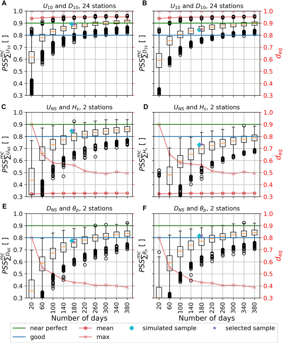
FIGURE 6. Same as Figure 3, but for (A,B) the projected two-dimensional distributions 10-m wind speed, U₁₀, and direction, D₁₀, (C,D) near-surface wind speed (U_NS) and significant wave height (H_s), and (E,F) near-surface wind direction (D_NS) and peak wave direction (τ_p).

The evaluation of different matrices shows that about 180 days should be considered to match the probability density functions of the long-term wind and wave climate in the German Bight. To reduce the computational costs to simulate those days, they were sampled as a 48-h consecutive period. Unfortunately, four 48-h periods out of the 90 periods could not be performed with the set-up described in Section 2.2. Thus, those 8 days could not be taken into account for the analysis in Section 3. However, the blue diamonds in Figures 3, 4, 6 for 172 days shows that the performance in terms of PSS is still comparable to 180 days and thus the simulated sample is still climatically representative.

FIGURE 7

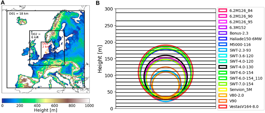
FIGURE 7. (A) Orography as used in the respective three nested domains. Orange dots are offshore wind turbines in the innermost domain. (B) Height of the vertical model levels at mass coordinates. Circles indicate the rotor area for the different offshore turbines.

2.2 Modeling System and Set-Up

We use the Coupled-Ocean-Atmosphere-Wave-Sediment Transport modeling system (COAWST, Warner et al., 2008; Warner et al., 2010) version 3.2 to simulate the selected days (Section 2.1). We enable the atmospheric Weather, Research and Forecasting model (WRF, Skamarock et al., 2008) version 3.7.1 and for some simulations the third generation spectral Simulation WAves Nearshore model (SWAN, Booij et al., 1999) v41.01AB. The other components of COAWST are not activated in this study.

The WRF and SWAN models are two-way coupled online using the Wave Boundary Layer Model (WBLM) implemented in SWAN (Du et al., 2017, 2019; Larsén et al., 2019). The WBLM considers the vertical change of stresses and energy in the wave boundary layer (WBL), which is the interface between the waves and the atmospheric boundary layer above. In the WBL, the wave induced stress, τ_w, is a significant component of the total stress τ_tot = τ_w + τ_t + τ_ν that consists also of the turbulent stress τ_t and the viscous stress τ_ν. However, τ_ν is negligible a few centimeters above the water surface. The WBLM solves this equation for τ_tot variation with height. In addition, it employs a conservation equation for the kinetic energy with height, ensuring that the momentum transfer between wind and waves is both flux and energy consistent. To ensure that the momentum lost from the atmosphere is exactly the same as the momentum gained by the waves, the wind-input source function and the dissipation function in SWAN are modified (Du et al., 2017, 2019). The wave growth function takes into account the local friction velocity, the phase speed and the wind-wave (mis-)alignment for all simulated frequencies and directions. Thus, it includes a more complete picture of wind-wave (mis-)alignment than the bulk parameterization approach by Porchetta et al. (2019), which only takes into account the misalignment between peak wave direction and wind direction. To solve the two conservation equations, the 10 m wind components are transferred to the SWAN-WBLM system. Using an iterative approach the corresponding surface roughness length z₀ is transferred back to the surface module of the WRF model. The exchange frequency is set to 6 min following Larsén et al. (2019).

To simulate the effects of wind farms on the atmospheric flow, two wind farm parameterizations (WFP) are employed: the scheme by Fitch et al. (2012) (termed FIT here) and the Explicit Wake Parameterization (EWP, Volker et al., 2015). These are the most commonly applied according to a review by Fischereit et al. (2021a) and differ with respect to the treatment of turbine-induced forces and turbine-induced TKE. The EWP considers a sub-grid scale vertical wake expansion, which is neglected in FIT. In the EWP, because shear is assumed to be the dominant source of TKE, turbine-induced TKE is not added. In contrast, the FIT scheme includes an explicit source term for turbine induced TKE. Here, we apply the FIT scheme with the bug-fix proposed by Archer et al. (2020) and a correction factor of 0.25 to adjust the magnitude of turbine-induced TKE. The initial length scale used in the EWP scheme to account for the subgrid scale wake expansion was set to 1.7. Volker et al. (2015) and Larsén and Fischereit (2021a) found very low sensitivity to values between 1.5 and 1.9 (1.7), respectively.

The effect of wind turbine poles on waves is not considered in this study. Based on the reviewed literature (Section 1), the impact of changed wind stress as captured through a WFP is larger than the impact of the poles in the far wake. Since near wakes cannot be captured in the mesoscale model, neglecting the impact of turbine poles is a valid assumption.

To include the effects of wind turbines in the simulation, their location, hub height, rotor diameter and power and thrust curves are required. We combined three different sources to create the data set of turbine locations for July 2020 as shown in Figure 7A: most German and Danish wind farms were taken from Bundesnetzagentur (2022) and Energistyrelsen (2020), respectively. Other wind farms, which were not included in these two data sets, use turbine locations derived from SAR images in Langor (2019) and have been manually corrected to fit the wind farm shapes and turbine numbers from EMODnet (Emodnet, 2020b). This method was also applied in Larsén and Fischereit (2021a). Some of the thrust and power curves correspond to the actual turbine curves (Supplementary Table S3) and were taken from Larsén and Fischereit (2021b). For the Alpha Ventus and BARD Offshore wind farms, the thrust and power coefficients are not publicly available; we used the power and thrust curves of M5000-116 that are scaled from the NREL 5 MW turbine. The Senvion 6.2M126 turbine in the Nordsee One, OWP Nordergründe and OWP Nordsee Ost wind farms were similarly scaled from the DTU 10 MW reference turbine. For the Haliade150-6 MW turbine the power and thrust curves of SWT-6.0–154 is used for the same reason. More details are given in Larsén and Fischereit (2021a).

The review in Fischereit et al. (2021a) found that the simulation results with WFP are sensitive to the choice of horizontal and especially to vertical resolution in the atmospheric model. Here, we follow the recommendations derived in Fischereit et al. (2021a) and use a horizontal grid spacing of the innermost domain of 2 km × 2 km (Figure 7A) and a vertical resolution of about 10 m up to 250 m, i.e. 50 m above the highest rotor (Figure 7B), and total of 62 vertical levels. The model SWAN uses the same horizontal model grid as the WRF model; and following Larsén et al. (2019), we choose 61 frequencies and 36 directional bins with a minimum frequency of 0.03 Hz. More details on the model set-ups, including the parameterizations used, are given in the Supplementary Table S2.

The coupled modelling system is integrated for 60 h, which includes 12 h of spin-up time and 48 h of actual simulation time covering the 86 pairs of selected sample days (Section 2.1). The ERA5 (Hersbach et al., 2018) and OSTIA sea surface temperature (Donlon et al., 2012) are used as initial and boundary conditions for the WRF simulations. Following the approach in Larsén et al. (2019), the SWAN model is initialised with the output spectrum of a previous 24-h long uncoupled SWAN simulation prior to the spin-up of the coupled simulations. The ERA5 10-m winds are used as forcing for these uncoupled simulations. For more details see Supplementary Table S2.

Simulations of different complexity are performed to address the research questions. The base set is the uncoupled stand-alone atmosphere model simulations with the WRF model without wind farms (called WRF in the following). We perform simulations with parameterized wind farms with the FIT (WRF + FIT) and the EWP (WRF + EWP) schemes. The coupled simulations conducted to better take into account the wind-wave-wake interaction are: (WRF + SWAN) and with parameterized wind farms (WRF + SWAN + FIT). The differences among these five sets of simulations will be used to address the research questions (Section 1).

2.3 Statistical Analysis

The simulations will be analysed based on climatic means of the scenarios for different parameters x. The climatic mean is derived as the average over 86 48-hour-long simulations. The absolute difference of the climatic mean of two scenarios S1 and S2 is normalized by the subtrahend to derive a relative difference of the climatic means between two scenarios: $({\bar{x}}_{S1}-{\bar{x}}_{S2})/{\bar{x}}_{S2}$. This metric can be interpreted as a relative BIAS. The standard deviation, σ, of the difference of the 86 means at each grid point is used complimentary to characterize the spread of the differences.

The statistical significance of the difference between the scenarios is derived through a t-test: Each simulation is averaged over 48 h to ensure that samples are uncorrelated. For each grid point the hypothesis is tested, whether the mean difference between the 86 means is significant different from zero using a one sample two-sided t-test. A p-value of 0.01 is chosen, which provides a “strong” evidence according to Wilks (2019).

To evaluate the model performance against measurements, the average difference (BIAS) is used to evaluate the systematic part of the error. The Root Mean Square Error (RMSE) is used complementary as a error measure for the combined systematic and non-systematic error. The correlation coefficient (r) evaluates the correct timing of the simulations. Detailed equations for the error measures are given for instance in Schlünzen and Sokhi (2008).

3 Results

In Section 3.1 the simulation results are evaluated against measurements. The impacts of the wind-wave-wake interactions derived from the statistical downscaling method are shown in Section 3.2 and Section 3.3 for the hub-height wind and wave climate, respectively.

3.1 Evaluation of the Modelling System Performance

To evaluate the overall performance of the modelling system, WRF + SWAN and WRF simulations (see Section 2.2 for the abbreviations) are compared against different observations around the German Bight (Figure 2). The same stations as in Figures 3, 5, respectively, are used for 10-m wind speed (U₁₀), significant wave height (H_s) and wind speed interpolated to 100 m height (U₁₀₀). The scatter plots of measurements versus simulation interpolated to the different measurement locations for the three parameters along with performance measures are shown in Figure 8. The analysis of H_s for HelgolandWR is not included because the interpolation to the measurement location involved a land point.

FIGURE 8

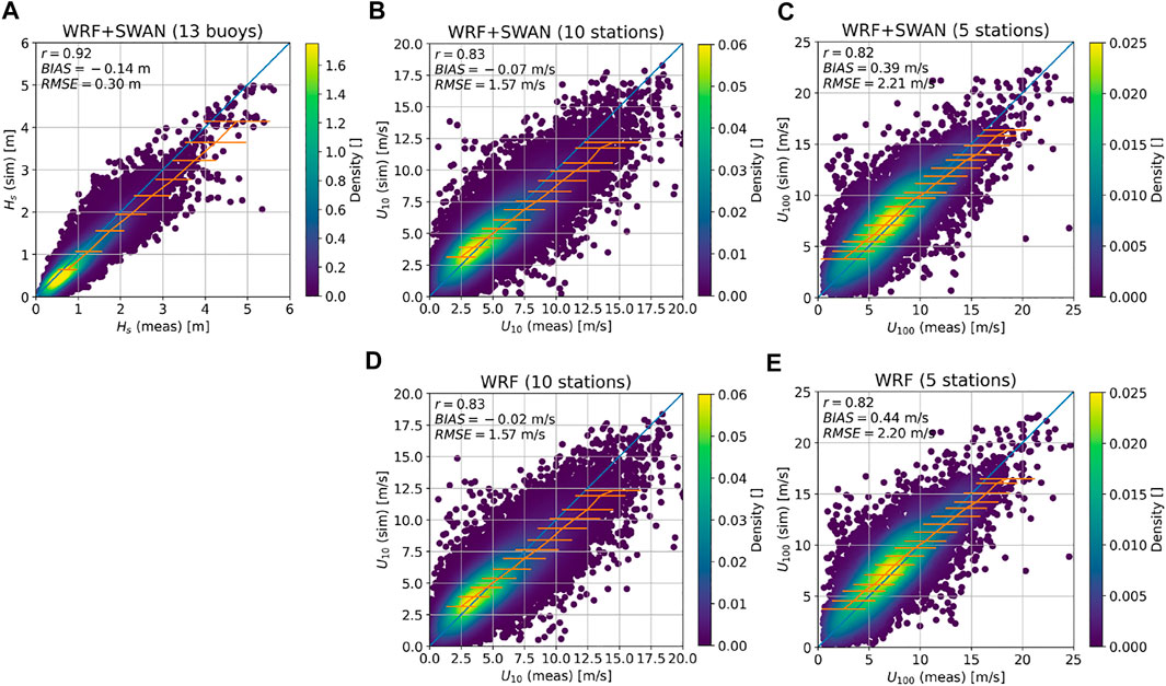
FIGURE 8. Overall evaluation of (A) significant wave height H_s (B,D) 10-m wind speed U₁₀ and (C,E) 100-m wind speed U₁₀₀ for (A–C) WRF + SWAN and (D,E) WRF against observations from different stations around the German Bight. The orange line shows mean and standard deviations for different classes. r is the correlation coefficient.

Overall all three parameters are well simulated with high correlation coefficients between 0.82 and 0.92 and relatively low biases. On average H_s is slightly underestimated, while U₁₀ and U₁₀₀ are overestimated for lower wind speeds and underestimated for higher wind speeds.

The results for WRF + SWAN (Figure 8B,C) and stand-alone WRF (Figure 8D,E) perform equally well. Thus, contradictory to simulations with very high wind speeds during storms done by Larsén et al. (2019), the uncoupled modelling system performs comparable well for the wind speed range up to 20 m s⁻¹ based on these error measures.

The average wind speed per bin for WRF + SWAN and WRF for wind speed between 5 m s⁻¹ and 20 m s⁻¹ (Figure 8B–E orange line), indicates consistently smaller wind speeds in WRF + SWAN compared to WRF. This is due to higher surface roughness lengths z₀ in this wind speed range calculated through the WBLM in SWAN compared to WRF (Supplementary Figure S7). However, the results from the measurement campaigns CBLAST (Edson et al., 2013) and COARE (Fairall et al., 2003) lie still within one standard deviation of the coupled model results. The COARE experiment is the basis for the Charnock-based relationship used in WRF. Larsén et al. (2019) showed similar findings for another independent set of days and Wu et al. (2020) noticed the same trend of smaller wind speeds in the coupled simulations for moderate wind speed in summer in their coupled modelling system, which uses a different atmosphere and wave model than the COAWST system. Therefore, the coupled simulation results are deemed reasonable, however, possible improvements within this wind speed range for the WBLM could be considered in the future.

The BIAS, RMSE and r provide some insight into the model performance, but they do not evaluate how well the PDF for each variable is simulated. This can be done using the PPS introduced in Section 2.1. Following the same calculations PSS and PSS^mc are derived from WRF and WRF + SWAN for the different variables in Figures 3, 4. Those values are shown as filled triangles for WRF + SWAN and as empty triangles for WRF in the respective figures. Triangles pointing to the left or down refer to PSS, while triangles pointing the right or up refer to PSS^mc, i.e. only the time span of the measurement climate at that station is considered. As for the previous evaluation analysis, H_s is calculated from the simulations based on only 13 stations.

The PSS or the PSS^mc from WRF + SWAN and WRF show mostly comparable scores to the predicted score based on measurements (simulated sample, blue diamond), except for U₁₀, H_s and θ_p. However, also for those variables, the skill score is still close to good or better. When considering all days for H_s and θ_p, instead of just the period where measurements are available at the different stations, more of the PDF variability is captured. This indicates that some of the missing variability during the measurement period can be captured through the variability on other days.

Comparing PSS or the PSS^mc for WRF + SWAN and WRF for U₁₀, U₁₀₀, D₁₀ and D₁₀₀ shows again comparable skill to capture the PDFs for both the uncoupled and the coupled simulations. The scores for individual stations (not shown), indicate that for some stations the coupled system performs slightly better, while for other stations the uncoupled system performs slightly better. Overall the coupled system performs better at more stations for U₁₀, while the uncoupled system performs better at more stations for the other variables.

3.2 Impacts on Hub-Height Wind

3.2.1 Impacts of Wind Farms

The 2020 built-out of OWFs clearly has an impact on the available wind resources. Figure 9 shows the simulated wind climate at 100 m height for A) the uncoupled simulation using WRF-only and D) the coupled simulation using the WRF and SWAN models. The relative differences in wind speed (Figures 9B,C,E) due to the presence of wind farms as seen in the different scenarios by subtracting the no-wind-farm scenario from the respective wind farm scenario and normalizing the difference using the no-wind-farm scenario.

FIGURE 9

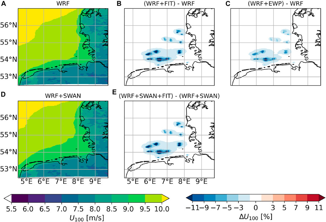
FIGURE 9. (A,D) Simulated long-term mean wind speed at 100 m height for (A) WRF and (D) WRF + SWAN and (B,C,E) relative reduction of wind speed based on (B) (WRF + FIT)-WRF, (C) (WRF + EWP)-WRF and (E) (WRF + SWAN + FIT)-(WRF + SWAN) all normalized by the respective subtrahend.

Wind speed reductions are on average about 10% or about 2 m s⁻¹ close to the wind farm and are reduced with increasing distance. This is because the wind speed is reduced at the grid cells where turbines are present, but the wind deficits recover with increasing distance though turbulent mixing. Some groups of wind farms act like a wind farm cluster, meaning that there is a continuous wind speed deficit $>1$ % linking the individual farms. For FIT three such cluster areas are visible in the German Bight, while for EWP five clusters are simulated.

The magnitude of the wind speed deficit depends on the chosen WFP and the model complexity (coupled or uncoupled). It amounts to a maximum of −21.7% for WRF + FIT, −13.3% for WRF + EWP and −22.1% for WRF + SWAN + FIT. Thus, the maximum wind deficit for EWP is just 61% of the maximum wind deficit for FIT at 100 m height. The lower wind speed deficit for EWP is in line with previous studies (Pryor et al., 2020; Shepherd et al., 2020; Fischereit et al., 2021b). The maximum deficits for WRF + SWAN + FIT is 1% smaller than for WRF + FIT, which is discussed in more detail in Section 3.2.2.

The extent of the wake affected area is also important for wind energy planning, since it indicates the impact of one wind farm on the surrounding farms. Following Pryor et al. (2020), we define the wake affected area A_2% as the area where the velocity deficit is greater than 2%. The respective areas for the scenarios are A_{2%,(WRF+FIT)−WRF} = 9,052 km², A_{2%,(WRF+EWP)−WRF} = 6,488 km² and A_{2%,(WRF+SWAN+FIT)−(WRF+SWAN)} = 9,024 km². Thus, the A_{2%,(WRF+EWP)−WRF} is only 72% of A_{2%,(WRF+FIT)−WRF}. This ratio is slightly larger than the ratio between EWP and FIT that Pryor et al. (2020) estimated for the US mid-west. However, the same trend of larger wake-affected areas for FIT than for EWP is seen. The higher value in our study could be both due to the offshore location or because the simulations in Pryor et al. (2020) do not take into account the bug-fix by Archer et al. (2020).

The influence of the model complexity is smaller on average than the influence of the chosen WFP on the wake affected area. The wake affected areas of both the coupled and uncoupled simulations are comparable, although it is slightly smaller in the coupled simulations. The reason for smaller wake affected area is the higher mixing in the coupled simulations, which is reflected in up to 6% higher values of TKE in 100 m height in the coupled simulations (TKE₁₀₀, Figure 10E,F). Those higher TKE₁₀₀ are a consequence of higher TKE at 10 m (Supplementary Figure S8), which is related to the higher surface roughness lengths calculated in the coupled simulations (Section 3.1).

Defining A_5% and A_10% accordingly to A_2%, results in A_{5%,(WRF+FIT)−WRF} = 3,028 km², A_{10%,(WRF+FIT)−WRF} = 1092 km² and A_{5%,(WRF+SWAN+FIT)−(WRF+SWAN)} = 3,036 km², A_{10%,(WRF+SWAN+FIT)−(WRF+SWAN)} = 1112 km², respectively. Thus, the wake affected area decreases with increasing wind speed deficit threshold more in the coupled simulations than in the uncoupled ones. This agrees with the previous finding that the maximum wind speed deficit is larger in the coupled simulations and will be discussed in more detail in Section 3.2.2.

The climatic mean impact of neighbouring wind farms on wind speed at 100 m (Figure 9) indicates the expected magnitude of losses from other farms. These losses vary with time as shown by the standard deviation of the wind speed difference over the 86 48-means (Supplementary Figure S9). Like the mean difference, the standard deviation of the differences also decreases with increasing distance to the farms.

A t-test is performed to derive where the difference is statistically significant. Supplementary Figure S10B,E,H,K shows exemplary for four sites (Supplementary Figure S10C,F,I,L) the difference distributions between WRF + FIT and WRF along with the derived p-values for the t-test described in Section 2.3. The selected sites illustrate the narrowing of the difference distribution with increasing distance from the farms and the corresponding increase in p-values. Supplementary Figure S11 shows the area of significant differences based on p < 0.01 as dotted hatched area. Regardless of the chosen WFP, the area of significant differences connects all offshore farms in the German Bight. This indicates that already with the 2020 built-out, the wind farms in the German Bight influence each other’s wind resources.

FIGURE 10

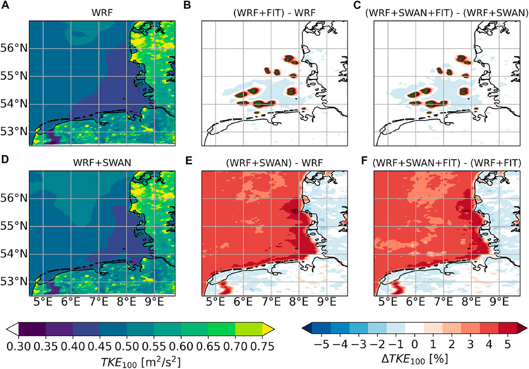
FIGURE 10. (A,D) Simulated long-term TKE at 100 m height for (A) WRF and (D) WRF + SWAN and (B,C,E,F) relative reduction of wind speed based on (B) (WRF + FIT)-WRF, (C) (WRF + SWAN + FIT)-(WRF + SWAN), (E) (WRF + SWAN)-(WRF) and (F) (WRF + SWAN + FIT)-(WRF + FIT) all normalized by the respective subtrahend.

3.2.2 Impacts of Waves

Hub-height wind speed is reduced by on average 1% (or about 0.15 m s⁻¹) above the sea (Figure 11B), with a more realistic representation of wind-wave interaction in the coupled simulations. This is due to the higher roughness length z₀ in the wind speed range 5 m s⁻¹ to 20 m s⁻¹ calculated through the WBLM in the SWAN model compared to the Charnock-based relationship used in the WRF model (Section 3.1). Thus, compared to the impact of neighbouring wind farms (Section 3.2.1), the mean impact of waves is smaller. Also the standard deviation of the 48-h mean wind speed difference between the uncoupled and coupled simulation (Supplementary Figure S12) is smaller than the difference between simulation with and without wind farms (Supplementary Figure S9). However, the impact of a more realistic representation of wind-wave interaction in the coupled simulations is not concentrated in a particular area, but spread out over the entire model area. Thus, average differences are also significant over larger areas, in particular offshore (Supplementary Figure S13).

FIGURE 11

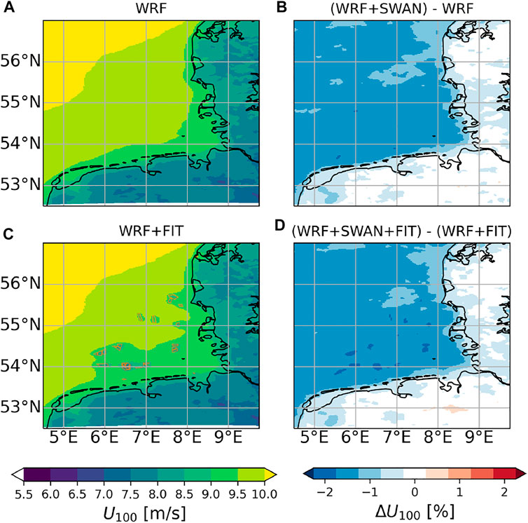
FIGURE 11. (A,B) Simulated long-term wind speed at 100 m height for (A) WRF and (C) WRF + FIT and (B,D) relative reduction of wind speed based on (B) (WRF + SWAN)-WRF and (D) (WRF + SWAN + FIT)-(WRF + FIT) both normalized by the respective subtrahend.

Despite the average reduction in Figure 11 being small, there is a huge spread in wind speed difference due to coupling for each 10 min-period. Figure 12 shows the histogram of grid point differences between WRF + SWAN and WRF over the analysed area in Figure 9 for every 10 min-period of the 172 days. Simulated wind speeds between the coupled and uncoupled simulations can differ by more than ±20% or ±2 m/s on a 10 min time scale, respectively. The mean difference between WRF + SWAN and WRF over the entire analysed area is almost zero, but slightly skewed towards negative values due to the increased drag by the waves (Section 3.1). Differences are positive more often onshore than offshore, which means that for the coupled simulations wind resources at hub height are more often increased onshore than offshore. However, those more positive 10-min-fluctuations do not manifest in statistically significant differences of the climatic means onshore (Supplementary Figure S11) and thus should be treated with caution. The relative differences are strongly influenced by outliers due to small wind speeds in WRF, which are used for normalization. Thus, the positive means for the relative differences for “onshore” and “all” are artifacts of those outliers. Medians, being less affected by outliers, are negative for all areas (dotted lines).

FIGURE 12

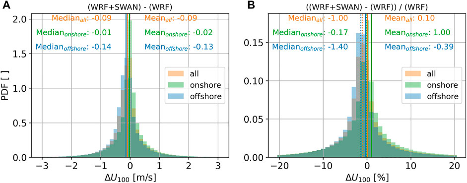
FIGURE 12. Histogram of simulated relative U-difference at 100 m height for (A) the absolute difference (WRF + SWAN)-(WRF) and (B) the relative difference ((WRF + SWAN)-(WRF))/(WRF) over the entire analysed area shown in Figure 9 (orange) and for the respective offshore and onshore areas only (blue and green, respectively). Solid lines show mean differences and dotted lines median difference.

Wind-wave-wake interactions lead to an additional reduction in hub-height wind speed on average in the coupled simulations compared to the uncoupled ones in most wind farms (Figure 11D). Although some areas outside of the wind farms also show reductions larger than 1.75%, the additional reduction is most systematic within the wind farms areas. The additional relative reduction is visible throughout the lower atmosphere, as shown by vertical profiles in and outside wind farms for (WRF + SWAN + FIT)-(WRF + FIT) Supplementary Figure S14C. The absolute difference for (WRF + SWAN + FIT)-(WRF + FIT) is larger outside the farms than inside up to 50 m height, when the difference outside the farms becomes larger (Supplementary Figure S14B). The additional reduction in the wind farms stems mostly from the non-linear dependence of the thrust coefficient (c_T) on wind speed: The slope of the average thrust coefficient over all farms correlates well with the difference in wind speed at 100 m height for (WRF + SWAN + FIT)-(WRF + FIT) between the mean over the center point of all wind farms and the mean over three sites outside wind farms (Supplementary Figure S15). Thus, the slightly smaller wind speeds in the coupled simulations due to the higher surface roughness (Section 3.1) cause higher c_T-values for the coupled simulations compared to the uncoupled simulations.

3.3 Impacts on Waves

The interaction between wind and waves can have multiple effects: the presence of waves impacts the wind resources (Section 3.2.2), but the presence of wind farms also impacts the waves. Through mixing of the wind speed deficits downwards, wind deficits are also present at 10 m (Supplementary Figure S16). Thus, wind turbines affect the energy transfer from the wind to the waves. The most notable effect is a reduction of the significant wave height H_s in the wind farm area (Figure 13).

FIGURE 13

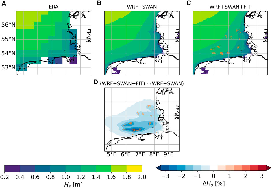
FIGURE 13. (A) Long-term significant wave height (H_s) from ERA5 and simulated by (B) WRF + SWAN and (C) WRF + SWAN + FIT. (D) Relative reduction on significant wave height from (WRF + SWAN + FIT)-(WRF + SWAN) normalized by (WRF + SWAN).

Figure 13A shows the averaged significant wave height H_s from the ERA5 reanalysis. The spatial pattern compares well with the pattern derived from WRF + SWAN (Figure 13B). The existing wind farms modify the wave climate slightly, by reducing H_s up to 3.5% in the wind farm area (Figure 13D). This reduction is comparable to the maximum reduction of 5% found by Christensen et al. (2013) close to a wind farm in idealised studies using an uncoupled wave model.

The significant wave height recovers with decreasing wind speed deficits with increasing distance from the farms (Figure 9). The area with a larger reduction than 2% amounts to A_{2%,(WRF+SWAN+FIT)−(WRF+SWAN)} = 2,248 km² and larger reductions than 1% to A_{1%,(WRF+SWAN+FIT)−(WRF+SWAN)} = 15,888 km², which indicates that the significant wave height recovers quite fast.

The wind farm impact on waves depends on the fetch. This is shown by the standard deviation of the difference in the 86 48-hour-means (Supplementary Figure S17), which is shifted west- and slightly northwards compared to the position of the wind farms. The area of statistical significant impact of wind farms based on a p-value of 0.01 extends even further west- and northwards (Supplementary Figure S18).

4 Discussions and Conclusions

We investigated climatic impacts of wind-wave-wake interactions in offshore wind farms in the German Bight. For that, we extended the measurement-driven statistical-dynamical downscaling method from Rife et al. (2013) and Boettcher et al. (2015) to simultaneously represent the 30-years average wind and wave climate. We concluded that about 180 days are necessary to represent the wind and wave climates and their relations with sufficient accuracy based on the PSS (Perkins et al., 2007).

To isolate the impacts of the wind, wave and wake interactions, we simulated the representative days with model set-ups of different complexity. We performed stand-alone uncoupled atmospheric simulations with and without wind farms and two different WFPs using the modelling system COAWST (Warner et al., 2008; Warner et al., 2010). The coupled COAWST simulations used the WBLM (Du et al., 2017; Du et al., 2019) as an interface and we have performed simulations without wind farms and with one of the WFP schemes (FIT). We considered all offshore wind turbines that were present in July 2020 and used as far as possible realistic thrust and power curves for the different turbine models. Overall, both the uncoupled and coupled model simulations without wind farms performed satisfactory in terms of correlation coefficient, BIAS and RMSE as well as in terms of capturing the PDF as shown through the PSS. The difference between the various model set-ups allowed to address the two research questions (Sec. 1):

1. Wind farm wakes of neighbouring farms and waves affect the long-term wind resources offshore. It was shown that with the 2020 built-out in the German Bight, wind resources of neighbouring farms are reduced and that the individual farms start to act as a wind farm cluster consisting of several farms. The magnitude and extend of wind farm wakes on neighbouring wind resources depends on the WFP and on the model complexity.

• The simulations using the EWP scheme show in general smaller wind speed deficits, smaller wake-affected areas and smaller increases in TKE compared to simulations using the FIT scheme. This is in line with previous investigations (Pryor et al., 2020; Shepherd et al., 2020; Larsén and Fischereit, 2021a; Fischereit et al., 2021b). Thus, by using two WFPs an ensemble of possible impacts can be constructed.

• In the coupled simulations, average hub-height wind speeds are smaller, maximum wind speed deficits in the wind farm are slightly larger, wake-affected areas smaller and TKE values are higher compared to the uncoupled simulations. The reason for these impacts is higher surface roughness lengths derived from the WBLM in the investigated wind speed range compared to the Charnock-based parameterization in the uncoupled simulations. The higher roughness reduces the average wind speed and creates more vertical mixing, which reduces the wake affected area. In conclusion, including a wave impact in the modeling causes on average stronger wind speed deficits in the farm that recover faster outside the farm. Although the magnitude of the average impact is small, wind speed difference between the coupled and uncoupled simulation can be larger than ±20%.

2. Significant wave heights are reduced in the area of the wind farms by up to 3.5% for the 2020 built-out of OWFs and thus agree well with the results from the idealized study by Christensen et al. (2013). The wave power depends quadratically on the significant wave height (Glendenning, 1977). Thus, OWF could help to reduce coastal erosion just like wave farms as suggested by Rodriguez-Delgado et al. (2019). While the effect is currently small during specific situations or with future built-outs of OWFs (BSH, 2021) this might become relevant. In addition, OWFs can aid coastal protection through reduced wind speeds and precipitation as shown in Pan et al. (2018).

The measurement-driven statistical downscaling approach has the advantage of being independent of inherent biases in relatively coarse reanalysis products. However, offshore measurements are sparse (Veers et al., 2019) and often relatively short. Here, we solved this problem by defining a base sample for 10-m wind measurements first, since long records exist for these standard WMO measurements. Based on the so-called measurement climate at each station for each variable, the representativity for the other variables were derived. Reanalysis data was used to confirm the selection and showed no systematic bias due to the selection based on the measurement climates. To transfer this statistical downscaling approach to other areas with fewer measurement stations, reanalysis data could indeed be used such as done in the approach by Rife et al. (2013). However, using a multi-location approach and considering the representativity of relationships between variables as done in the present method is highly recommended. The methodology can be adapted to future climate scenarios using climate projections data.

The evaluation of the simulations cannot conclude whether the coupled or uncoupled modelling system provides more accurate results, because the performance varied between stations and variables. The performance of a particular set-up could also depend on the atmospheric or sea state, which should be investigated in the future. Furthermore, part of the measurements are affected by wind farm wakes themselves, which complicate the comparisons. Nevertheless, the simulations showed significantly different surface roughness lengths in the coupled and uncoupled system, and that those differences affect the wind resources.

The difference in surface roughness lengths in the coupled and uncoupled simulations stems from the on average young wave age in the area of the German Bight. Supplementary Figure S19A shows the average inverse wave age, U₁₀/c_p, where c_p is the wave phase velocity at the wave peak frequency. According to Cifuentes-Lorenzen et al. (2013), U₁₀/c_p > 0.82 characterizes young waves. Thus, on average waves are young in the analysed area of the German Bight. In addition, wind and waves are on average not fully aligned. Supplementary Figure S19B shows the angle between D₁₀ and θ_p, which is between 10° and 50°, depending on the outer or inner area of the German Bight. This misalignment is taken into account in the roughness length estimation in the WBLM. The roughness length parameterization (Fairall et al., 2003) in the WRF model, as being a function of wind speed alone and calibrated for the open sea (deep water) area, cannot capture the full drag induced by the waves on the atmosphere.

On a climatic average, wind-wave interaction in the coupled modelling reduces the wind resources due to the increased drag. While the magnitude of the average wind speed difference between the coupled and uncoupled simulations is small, the impacts on wind power potential might be larger due to the non-linear dependence of power on wind speed. This should be investigated in future studies. In addition, while on average wind speeds decrease, for particular regions and time periods, coupling can also increase wind speeds (Figure 12). Overall, the differences due to wind-wave interaction can be ±20%. This magnitude of wind speed variation agrees well with the study by Porchetta et al. (2021) for the German Bight. They identified wind-wave misalignment as an important driver for the difference. However, other parameters, such as atmospheric stability, wind speed or wave age could also play a role. In future studies, the performed simulations could be analysed based on these parameters, to clarify the most important coupling mechanisms in the German Bight area.

The climatic impact on waves can be different for other wind directions with larger fetches and older seas. Christensen et al. (2013) concluded that for short fetches (10–20 km) and moderate wind speeds (10 m s⁻¹) the effect is largest, since the wind and wave field is not yet in balance. Thus, compared to the average climatic impact of 3.5% determined here, the significant wave height deficit could be less from westerly and north-westerly directions and stronger for other directions. More in-depth analysis on how wind farms impact other parameters beside significant wave height (e.g., wave period and peak direction) should be performed in the future, follow up on Christensen et al. (2013) conclusions that wind farms have little effect on wave periods. Furthermore, wave spectra could be analysed to investigate the impact of wind farms on other parts of the spectrum following up on Bärfuss et al. (2021). A better understanding on the wave impact is necessary, since energy input though waves affects the ocean mixing and thus life in the sea (Jenkins et al., 2012; Carpenter et al., 2016). In addition, co-locating OWF and wave farms for maximising renewable energy harvesting are explored (Pérez-Collazo et al., 2015) and thus an accurate understanding of wind-wave-wake interaction is important.

Swell waves are partly accounted for through the nesting approach taken in this study. However, considering the importance of swell-wind interaction found in LES studies (Yang et al., 2014; AlSam et al., 2015), the consideration of swell in the WBLM should be improved in the future. Furthermore, Wu et al. (2020) showed that not only wind-wave interaction, but especially ocean-atmosphere interaction have an impact on wind resources. On the other side, wind farms have been shown to impact ocean dynamics and stratification (Christiansen et al., 2022), which potentially causes adverse environmental effects (Farr et al., 2021). Thus, applying a fully coupled modelling system consisting of atmosphere, wave, ocean and wind farm parameterizations could help us understand the full spectrum of coupling mechanisms in the marine environment where wind farms are being build.

Data Availability Statement

The raw data supporting the conclusions of this article will be made available by the authors, without undue reservation.

Author Contributions

JF: Conceptualization, Methodology, Investigation, Writing–original draft, Writing–review and editing. AH: Discussing results, Writing–review and editing. XL: Discussing results, Writing–review and editing.

Funding

This study was partly funded by ForskEL/EUDP through the OffshoreWake project (PSO-12521/EUDP 64017–0017) and by Independent Research Fund Denmark through the “Multi-scale Atmospheric Modeling Above the Seas” (MAMAS) project (nr. 0217-00055B).

Conflict of Interest

The authors declare that the research was conducted in the absence of any commercial or financial relationships that could be construed as a potential conflict of interest.

Publisher’s Note

All claims expressed in this article are solely those of the authors and do not necessarily represent those of their affiliated organizations, or those of the publisher, the editors and the reviewers. Any product that may be evaluated in this article, or claim that may be made by its manufacturer, is not guaranteed or endorsed by the publisher.

Acknowledgments

We would like to thank Mark Kelly for the discussion on the statistical matrices and Jake Badger for his comments in the early stage of this work. The tall mast data used in this study have been kindly provided by the following people and organizations: Cabauw data were provided by the Cabauw Experimental Site for Atmospheric Research (Cesar), which is maintained by KNMI; The Hamburg Weather Mast data were provided by Ingo Lange; FINO1 and FINO3 data were made available by the FINO (Forschungsplattformen in Nord-und Ostsee) initiative, which was funded by the German Federal Ministry of Economic Affairs and Climate Action (BMWK) on the basis of a decision by the German Bundestag, organised by the Projekttraeger Juelich (PTJ) and coordinated by the German Federal Maritime and Hydrographic Agency (BSH). Data processing and visualization for this study was in part conducted using the python programming language and involved use of the following software packages: NumPy (van der Walt et al., 2011), pandas (McKinney, 2010), xarray (Hoyer and Hamman, 2017), Matplotlib (Hunter, 2007), cartopy (Met Office, 2015), Seaborn (Waskom, 2021), scikit-learn (Pedregosa et al., 2011) and SciPy (Virtanen et al., 2020). The authors are grateful for the tools provided by the open-source community. Some data used in this study was made available by the EMODnet Physics and the EMODne Human Activities project, www.emodnet-physics.eu/map (last accessed: 01.02.2022) and https://www.emodnet-humanactivities.eu/ (last accessed: 17.02.2022), respectively, funded by the European Commission Directorate General for Maritime Affairs and Fisheries. Deutscher Wetterdienst is acknowledged for the station data taken from the Climate Data Center (https://opendata.dwd.de). Danish Meteorological Institute (DMI) is acknowledged for the station data taken from the open data platform (www.DMI.dk/friedata).

Supplementary Material

The Supplementary Material for this article can be found online at: https://www.frontiersin.org/articles/10.3389/fenrg.2022.881459/full#supplementary-material

References

Alari, V., and Raudsepp, U. (2012). Simulation of Wave Damping Near Coast Due to Offshore Wind Farms. J. Coastal Res. 279, 143–148. doi:10.2112/JCOASTRES-D-10-00054.1

CrossRef Full Text | Google Scholar

AlSam, A., Szasz, R., and Revstedt, J. (2015). The Influence of Sea Waves on Offshore Wind Turbine Aerodynamics. J. Energ. Resour. Technol. Trans. ASME 137, 1–10. doi:10.1115/1.4031005

CrossRef Full Text | Google Scholar

Archer, C. L., Wu, S., Ma, Y., and Jiménez, P. A. (2020). Two Corrections for Turbulent Kinetic Energy Generated by Wind Farms in the WRF Model. Mon Weather Rev. 148, 4823–4835. doi:10.1175/MWR-D-20-0097.1

CrossRef Full Text | Google Scholar

Bärfuss, K., Schulz-Stellenfleth, J., and Lampert, A. (2021). Marine Science and Engineering the Impact of Offshore Wind Farms on Sea State Demonstrated by Airborne LiDAR Measurements. Jmse 9, 644. doi:10.3390/jmse9060644

CrossRef Full Text | Google Scholar

Banks, D. L., and Fienberg, S. E. (2003). “Data Mining, Statistics,” in Encyclopedia of Physical Science and Technology (New York: Elsevier), 247–261. doi:10.1016/b0-12-227410-5/00164-2

CrossRef Full Text | Google Scholar

Boettcher, M., Hoffmann, P., Lenhart, H.-J., Schlünzen, K. H., and Schoetter, R. (2015). Influence of Large Offshore Wind Farms on North German Climate. metz 24, 465–480. doi:10.1127/metz/2015/0652

CrossRef Full Text | Google Scholar

Booij, N., Ris, R. C., and Holthuijsen, L. H. (1999). A Third-Generation Wave Model for Coastal Regions: 1. Model Description and Validation. J. Geophys. Res. 104, 7649–7666. doi:10.1029/98JC02622

CrossRef Full Text | Google Scholar

BSH (2020). [Dataset]. FINO-datenbank. Available at: http://fino.bsh.de/ (Accessed 06 26, 2020).

Google Scholar

BSH (2021). Vorentwurf Flächenentwicklungsplan. Technical report. Hamburg: Bundesamt für Seeschiffahrt und Hydrographie. Available at: https://www.bsh.de/DE/THEMEN/Offshore/Meeresfachplanung/Flaechenentwicklungsplan/_Anlagen/Downloads/FEP_2022/Vorentwurf_FEP.pdf;jsessionid=E10149D8E4E444564919AD4D2F8F279D.live21301?__blob=publicationFile&v=2 (Accessed April 11, 2022).

Google Scholar

Bundesnetzagentur (2022). Marktstammdatenregister. Available at: https://www.marktstammdatenregister.de/MaStR (Accessed 03 19, 2021).

Google Scholar

Carpenter, J. R., Merckelbach, L., Callies, U., Clark, S., Gaslikova, L., and Baschek, B. (2016). Potential Impacts of Offshore Wind Farms on North Sea Stratification. PLoS ONE 11, e0160830. doi:10.1371/journal.pone.0160830

PubMed Abstract | CrossRef Full Text | Google Scholar

Chávez-Arroyo, R., Fernandes-Correia, P., Lozano-Galiana, S., Sanz-Rodrigo, J., Amezcua, J., and Probst, O. (2018). A Novel Approach to Statistical-Dynamical Downscaling for Long-Term Wind Resource Predictions. Met. Apps 25, 171–183. doi:10.1002/met.1678

CrossRef Full Text | Google Scholar

Christensen, E. D., Johnson, M., Sørensen, O. R., Hasager, C. B., Badger, M., and Larsen, S. E. (2013). Transmission of Wave Energy through an Offshore Wind Turbine Farm. Coastal Eng. 82, 25–46. doi:10.1016/j.coastaleng.2013.08.004

CrossRef Full Text | Google Scholar

Christiansen, N., Daewel, U., Djath, B., and Schrum, C. (2022). Emergence of Large-Scale Hydrodynamic Structures Due to Atmospheric Offshore Wind Farm Wakes. Front. Mar. Sci. 9, 1–17. doi:10.3389/fmars.2022.818501

PubMed Abstract | CrossRef Full Text | Google Scholar

Cifuentes-Lorenzen, A., Edson, J. B., Zappa, C. J., and Bariteau, L. (2013). A Multisensor from a Research Vessel during the Southern Ocean Gas Exchange experiment. J. Atmos. Oceanic Tech. 30, 2907–2925. doi:10.1175/JTECH-D-12-00181.1

CrossRef Full Text | Google Scholar

Deutscher Wetterdienst (2020). [Dataset]. Climate Data Center. Available at: https://opendata.dwd.de/climate_environment/CDC/observations_germany/climate/hourly/wind/historical/(Accessed 06 26, 2020).

Google Scholar

Díaz, H., and Guedes Soares, C. (2020). Review of the Current Status, Technology and Future Trends of Offshore Wind Farms. Ocean Eng. 209, 107381. doi:10.1016/j.oceaneng.2020.107381

CrossRef Full Text | Google Scholar

DMI (2020). [Dataset]. Danish Meteorological Institute - Open Data. Available at: https://confluence.govcloud.dk/display/FDAPI/Danish+Meteorological+Institute+-+Open+Data (Accessed 06 26, 2020).

Google Scholar

Donlon, C. J., Martin, M., Stark, J., Roberts-Jones, J., Fiedler, E., and Wimmer, W. (2012). The Operational Sea Surface Temperature and Sea Ice Analysis (OSTIA) System. Remote Sensing Environ. 116, 140–158. doi:10.1016/j.rse.2010.10.017

CrossRef Full Text | Google Scholar

Drennan, W. M. (2003). On the Wave Age Dependence of Wind Stress over Pure Wind Seas. J. Geophys. Res. 108, 8062. doi:10.1029/2000JC000715

CrossRef Full Text | Google Scholar

DTU (2020). [Dataset]. Rodeo Data. Available at: http://rodeo.dtu.dk/rodeo/ProjectListText.aspx?&Rnd=358938 (Accessed 02 16, 2022).

Google Scholar

Du, J., Bolaños, R., and Guo Larsén, X. (2017). The Use of a Wave Boundary Layer Model in SWAN. J. Geophys. Res. Oceans 122, 42–62. doi:10.1002/2016JC012104

CrossRef Full Text | Google Scholar

Du, J., Bolaños, R., Larsén, X. G., and Kelly, M. (2019). Wave Boundary Layer Model in SWAN Revisited. Ocean Sci. 15, 361–377. doi:10.5194/os-15-361-2019

CrossRef Full Text | Google Scholar

Edson, J. B., Jampana, V., Weller, R. A., Bigorre, S. P., Plueddemann, A. J., Fairall, C. W., et al. (2013). On the Exchange of Momentum over the Open Ocean. J. Phys. Oceanography 43, 1589–1610. doi:10.1175/jpo-d-12-0173.1

CrossRef Full Text | Google Scholar

Emodnet (2020a). [Dataset]. Physics. Available at: https://portal.emodnet-physics.eu/(Accessed 01 28, 2021).

Google Scholar

Emodnet (2020b). [Dataset]. Wind Farms (Polygons). Available at: https://www.emodnet-humanactivities.eu/search-results.php?dataname=Wind+Farms+(Polygons (Accessed 03 19, 2021).

Google Scholar

Energistyrelsen (2020). [Dataset]. Turbines Positions. Available at: https://ens.dk/service/statistik-data-noegletal-og-kort/data-oversigt-overene-rgisektoren (Accessed 03 19, 2021).

Google Scholar

Fairall, C. W., Bradley, E. F., Hare, J. E., Grachev, A. A., and Edson, J. B. (2003). Bulk Parameterization of Air-Sea Fluxes: Updates and Verification for the COARE Algorithm. J. Clim. 16, 571–591. doi:10.1175/1520-0442(2003)016<0571:bpoasf>2.0.co;2

CrossRef Full Text | Google Scholar

Farr, H., Ruttenberg, B., Walter, R. K., Wang, Y.-H., and White, C. (2021). Potential Environmental Effects of deepwater Floating Offshore Wind Energy Facilities. Ocean Coastal Manage. 207, 105611–105691. doi:10.1016/j.ocecoaman.2021.105611

CrossRef Full Text | Google Scholar

Ferčák, O., Bossuyt, J., Ali, N., and Cal, R. B. (2022). Decoupling Wind-Wave-Wake Interactions in a Fixed-Bottom Offshore Wind Turbine. Appl. Energ. 309, 118358. doi:10.1016/j.apenergy.2021.118358

CrossRef Full Text | Google Scholar

Fischereit, J., Brown, R., Larsén, X. G., Badger, J., and Hawkes, G. (2021a). Review of Mesoscale Wind-Farm Parametrizations and Their Applications. Boundary-layer Meteorol. 182, 175–224. doi:10.1007/s10546-021-00652-y

CrossRef Full Text | Google Scholar

Fischereit, J., Schaldemose Hansen, K., Larsén, X. G., van der Laan, M. P., Réthoré, P.-E., and Murcia Leon, J. P. (2021b). Comparing and Validating Intra-farm and Farm-To-Farm Wakes across Different Mesoscale and High-Resolution Wake Models. Wind Energ. Sci. Discuss. 2021, 1–31. doi:10.5194/wes-2021-106

CrossRef Full Text | Google Scholar

Fischereit, J., Larsén, X. G., and Hahmann, A. N. (2022). Documentation of the Model Setup for Climatic Impacts of Wind-Wave-Wake Interactions in Offshore Wind Farms. Zenodo. doi:10.5281/ZENODO.6225384

CrossRef Full Text | Google Scholar

Fitch, A. C., Olson, J. B., Lundquist, J. K., Dudhia, J., Gupta, A. K., Michalakes, J., et al. (2012). Local and Mesoscale Impacts of Wind Farms as Parameterized in a Mesoscale NWP Model. Monthly Weather Rev. 140, 3017–3038. doi:10.1175/MWR-D-11-00352.1

CrossRef Full Text | Google Scholar

Glendenning, I. (1977). Ocean Wave Power. Appl. Energ. 3, 197–222. doi:10.1016/0306-2619(77)90036-8

CrossRef Full Text | Google Scholar

Hahmann, A. N., Sīle, T., Witha, B., Davis, N. N., Dörenkämper, M., Ezber, Y., et al. (2020). The Making of the New European Wind Atlas - Part 1: Model Sensitivity. Geosci. Model. Dev. 13, 5053–5078. doi:10.5194/gmd-13-5053-2020

CrossRef Full Text | Google Scholar

Hersbach, H., Bell, B., Berrisford, P., Biavati, G., Horányi, A., Muñoz Sabater, J., et al. (2018). [Dataset]. ERA5 Hourly Data on Pressure Levels from 1979 to Present. Available at: https://cds.climate.copernicus.eu/cdsapp\#!/dataset/reanalysis-era5-pressure-levels (Accessed 19 03, 2021). doi:10.24381/cds.bd0915c6

CrossRef Full Text | Google Scholar

Hoyer, S., and Hamman, J. J. (2017). Xarray: N-D Labeled Arrays and Datasets in Python. J. Open Res. Softw. 5, 1–10. doi:10.5334/jors.148

CrossRef Full Text | Google Scholar

Hunter, J. D. (2007). Matplotlib: A 2D Graphics Environment. Comput. Sci. Eng. 9, 90–95. doi:10.1109/mcse.2007.55

CrossRef Full Text | Google Scholar

IOOS (2021). [Dataset]. IOOS QC: QARTOD and Other Quality Control Tests Implemented in Python, Ioos. Available at: github.io/ioos_qc/(Accessed 16 06, 2021).

Google Scholar

IRENA (2019). FUTURE of WIND Deployment, Investment, Technology, Grid Integration and Socio-Economic Aspects. Technical report. Available at: https://www.irena.org/-/media/Files/IRENA/Agency/Publication/2019/Oct/IRENA_Future_of_wind_2019.pdf (Accessed 03 22, 2021).

Google Scholar

Jenkins, A. D., Paskyabi, M. B., Fer, I., Gupta, A., and Adakudlu, M. (2012). Modelling the Effect of Ocean Waves on the Atmospheric and Ocean Boundary Layers. Energ. Proced. 24, 166–175. doi:10.1016/J.EGYPRO.2012.06.098

CrossRef Full Text | Google Scholar

Kalvig, S., Manger, E., Hjertager, B. H., and Jakobsen, J. B. (2014). Wave Influenced Wind and the Effect on Offshore Wind Turbine Performance. Energ. Proced. (Elsevier) 53, 202–213. doi:10.1016/j.egypro.2014.07.229

CrossRef Full Text | Google Scholar

Lange, I. (2020). [Dataset]. Wind- und Temperaturdaten vom Wettermast Hamburg des Meteorologischen Instituts der Universität Hamburg für den Zeitraum 2005 bis 2020. Personal communication on 2020-07-06.

Google Scholar

Langor, E. N. (2019). Characteristics of Offshore Wind Farm Wakes and Their Impact on Wind Power Production from Long-Term Modelling and Measurements. Technical report. Lyngby: DTU Wind Energy.

Google Scholar

Larsén, X. G., and Fischereit, J. (2021a). A Case Study of Wind Farm Effects Using Two Wake Parameterizations in the Weather Research and Forecasting (WRF) Model (V3.7.1) in the Presence of Low-Level Jets. Geosci. Model. Dev. 14, 3141–3158. doi:10.5194/gmd-14-3141-2021

CrossRef Full Text | Google Scholar

Larsén, X. G., Du, J., Bolaños, R., Imberger, M., Kelly, M. C., Badger, M., et al. (2019). Estimation of Offshore Extreme Wind from Wind‐wave Coupled Modeling. Wind Energy 22, 1043–1057. doi:10.1002/we.2339

CrossRef Full Text | Google Scholar

Larsén, X. G., and Fischereit, J. (2021b). A Case Study of Wind Farm Effects Using Two Wake Parameterizations in WRF (V3.7.1) in the Presence of Low Level Jets (Version 4) [Data set]. Zenodo. doi:10.5281/zenodo.4668613

CrossRef Full Text | Google Scholar

Leiding, T., Gates, L., Herklotz, K., Tinz, B., Rosenhagen, G., and Senet, C. (2016). Standardisierung und vergleichende Analyse der meteorologischen FINO-Messdaten FINO123 : Forschungsvorhaben FINO-Wind : Abschlussbericht : 12/2012-04/2016, Projektlaufzeit: 12/2012 bis 04/2016. Technical report. Hamburg: Deutscher Wetterdienst. Available at: https://www.tib.eu/de/suchen/id/TIBKAT%3A885536142 (Accessed April 11, 2022).

Google Scholar

Lyu, P., Park, S. G., Shen, L., and Li, H. (2018). “A Coupled Wind-Wave-Turbine Solver for Offshore Wind Farm,” in ASME 2018 1st International Offshore Wind Technical Conference, IOWTC 2018, San Francisco, CA, November 4–7, 2018 (American Society of Mechanical Engineers ASME). doi:10.1115/IOWTC2018-1046

CrossRef Full Text | Google Scholar

McKinney, W. (2010). “Data Structures for Statistical Computing in Python,” in Proceedings of the 9th Python in Science Conference, Austin, TX, June 28–July 3, 2010. Editors S. van der Walt, and J. Millman doi:10.25080/majora-92bf1922-00a

CrossRef Full Text | Google Scholar

Met Office (2015). Cartopy: A Cartographic python Library with a Matplotlib Interface. Exeter, Devon: Met Office.

Google Scholar

Pan, Y., Yan, C., and Archer, C. L. (2018). Precipitation Reduction during Hurricane Harvey with Simulated Offshore Wind Farms. Environ. Res. Lett. 13, 084007. doi:10.1088/1748-9326/aad245

CrossRef Full Text | Google Scholar

Paskyabi, M. B., Zieger, S., Jenkins, A. D., Babanin, A. V., and Chalikov, D. (2014). Sea Surface Gravity Wave-Wind Interaction in the Marine Atmospheric Boundary Layer. Energ. Proced. 53, 184–192. doi:10.1016/J.EGYPRO.2014.07.227

CrossRef Full Text | Google Scholar

Pérez-Collazo, C., Greaves, D., and Iglesias, G. (2015). A Review of Combined Wave and Offshore Wind Energy. Renew. Sust. Energ. Rev. 42, 141–153. doi:10.1016/j.rser.2014.09.032

CrossRef Full Text | Google Scholar

Pedregosa, F., Varoquaux, G., Gramfort, A., Michel, V., Thirion, B., Grisel, O., et al. (2011). Scikit-learn: Machine Learning in Python. J. Machine Learn. Res. 12, 2825–2830.

Google Scholar

Perkins, S. E., Pitman, A. J., Holbrook, N. J., and McAneney, J. (2007). Evaluation of the AR4 Climate Models' Simulated Daily Maximum Temperature, Minimum Temperature, and Precipitation over Australia Using Probability Density Functions. J. Clim. 20, 4356–4376. doi:10.1175/JCLI4253.1

CrossRef Full Text | Google Scholar

Ponce de León, S., Bettencourt, J. H., and Kjerstad, N. (2011). Simulation of Irregular Waves in an Offshore Wind Farm with a Spectral Wave Model. Continental Shelf Res. 31, 1541–1557. doi:10.1016/j.csr.2011.07.003

CrossRef Full Text | Google Scholar

Porchetta, S., Temel, O., Muñoz-Esparza, D., Reuder, J., Monbaliu, J., van Beeck, J., et al. (2019). A New Roughness Length Parameterization Accounting for Wind-Wave (Mis)alignment. Atmos. Chem. Phys. 19, 6681–6700. doi:10.5194/acp-19-6681-2019

CrossRef Full Text | Google Scholar

Porchetta, S., Muñoz-Esparza, D., Munters, W., van Beeck, J., and van Lipzig, N. (2021). Impact of Ocean Waves on Offshore Wind Farm Power Production. Renew. Energ. 180, 1179–1193. doi:10.1016/j.renene.2021.08.111

CrossRef Full Text | Google Scholar

Pryor, S. C., Shepherd, T. J., Volker, P. J. H., Hahmann, A. N., and Barthelmie, R. J. (2020). "Wind Theft" from Onshore Wind Turbine Arrays: Sensitivity to Wind Farm Parameterization and Resolution. J. Appl. Meteorology Climatology 59, 153–174. doi:10.1175/JAMC-D-19-0235.1

CrossRef Full Text | Google Scholar

Rife, D. L., Vanvyve, E., Pinto, J. O., Monaghan, A. J., Davis, C. A., and Poulos, G. S. (2013). Selecting Representative Days for More Efficient Dynamical Climate Downscaling: Application to Wind Energy. J. Appl. Meteorology Climatology 52, 47–63. doi:10.1175/JAMC-D-12-016.1

CrossRef Full Text | Google Scholar

Rodriguez-Delgado, C., Bergillos, R. J., and Iglesias, G. (2019). Dual Wave Farms for Energy Production and Coastal protection under Sea Level Rise. J. Clean. Prod. 222, 364–372. doi:10.1016/j.jclepro.2019.03.058

CrossRef Full Text | Google Scholar

K. H. Schlünzen, and R. S. Sokhi (Editors) (2008). Overview of Tools and Methods for Meteorological and Air Pollution Mesoscale Model Evaluation and User Training. GAW Report No. 181 (Geneva: World Meteorological Organization).

Google Scholar

Shepherd, T. J., Barthelmie, R. J., and Pryor, S. C. (2020). Sensitivity of Wind Turbine Array Downstream Effects to the Parameterization Used in WRF. J. Appl. Meteorology Climatology 59, 333–361. doi:10.1175/jamc-d-19-0135.1

CrossRef Full Text | Google Scholar

Skamarock, W. C., Klemp, J. B., Dudhia, J., Gill, D. O., Barker, D. M., Duda, M. G., et al. (2008). A Description of the Advanced Research WRF Version 3. Technical. Report. 2. Boulder: National Center for Atmospheric Research.

Google Scholar

van der Walt, S., Colbert, S. C., and Varoquaux, G. (2011). The NumPy Array: A Structure for Efficient Numerical Computation. Comput. Sci. Eng. 13, 22–30. doi:10.1109/MCSE.2011.37

CrossRef Full Text | Google Scholar

Veers, P., Dykes, K., Lantz, E., Barth, S., Bottasso, C. L., Carlson, O., et al. (2019). Grand Challenges in the Science of Wind Energy. Science 366, eaau2027. doi:10.1126/science.aau2027

PubMed Abstract | CrossRef Full Text | Google Scholar

Virtanen, P., Gommers, R., Oliphant, T. E., Haberland, M., Reddy, T., Cournapeau, D., et al. (2020). SciPy 1.0: Fundamental Algorithms for Scientific Computing in Python. Nat. Methods 17, 261–272. doi:10.1038/s41592-019-0686-2

PubMed Abstract | CrossRef Full Text | Google Scholar

Volker, P. J. H., Badger, J., Hahmann, A. N., and Ott, S. (2015). The Explicit Wake Parametrisation V1.0: a Wind Farm Parametrisation in the Mesoscale Model WRF. Geosci. Model. Dev. 8, 3715–3731. doi:10.5194/gmd-8-3715-2015

CrossRef Full Text | Google Scholar

Warner, J. C., Perlin, N., and Skyllingstad, E. D. (2008). Using the Model Coupling Toolkit to Couple Earth System Models. Environ. Model. Softw. 23, 1240–1249. doi:10.1016/j.envsoft.2008.03.002

CrossRef Full Text | Google Scholar

Warner, J. C., Armstrong, B., He, R., and Zambon, J. B. (2010). Development of a Coupled Ocean-Atmosphere-Wave-Sediment Transport (COAWST) Modeling System. Ocean Model. 35, 230–244. doi:10.1016/j.ocemod.2010.07.010

CrossRef Full Text | Google Scholar

Waskom, M. (2021). Seaborn: Statistical Data Visualization. Joss 6, 3021. doi:10.21105/joss.03021

CrossRef Full Text | Google Scholar

Wilks, D. S. (2019). “Frequentist Statistical Inference,” in Statistical Methods in the Atmospheric Sciences (Cambridge: Elsevier), 143–207. chap. 5. doi:10.1016/b978-0-12-815823-4.00005-5

CrossRef Full Text | Google Scholar

Wu, L., Shao, M., and Sahlée, E. (2020). Impact of Air-Wave-Sea Coupling on the Simulation of Offshore Wind and Wave Energy Potentials. Atmosphere 11, 327. doi:10.3390/atmos11040327

CrossRef Full Text | Google Scholar

Yang, D., Meneveau, C., and Shen, L. (2014). Effect of Downwind Swells on Offshore Wind Energy Harvesting - A Large-Eddy Simulation Study. Renew. Energ. 70, 11–23. doi:10.1016/J.RENENE.2014.03.069

CrossRef Full Text | Google Scholar

Zou, Z., Zhao, D., Zhang, J. A., Li, S., Cheng, Y., Lv, H., et al. (2018). The Influence of Swell on the Atmospheric Boundary Layer under Nonneutral Conditions. J. Phys. Oceanography 48, 925–936. doi:10.1175/JPO-D-17-0195.1

CrossRef Full Text | Google Scholar