Study on Trajectory Optimization of Hypersonic Vehicle Based on Neural Network

1 Introduction

Due to the outstanding tactical and technical advantages of hypersonic vehicles, they have received extensive attention. The horizontal take-off and landing of a high-speed cruise aircraft is usually powered by an air-breathing combined engine. During the climb, the acceleration and climb ability of the aircraft are affected and constrained by the dynamic characteristics, and the change in the flight profile will affect the engine performance. At the same time, the aerodynamic performance of the full mission profile is highly coupled with the engine performance (Wei, 2022). Therefore, flight profile design and optimization are very important for aircraft/engine matching and the overall technical scheme of aircraft (Mei et al., 2019), which is one of the research hotspots.

Trajectory optimization of a hypersonic vehicle involves many constraints and is a complex nonlinear multi-constraint optimal control problem (Gath and Calise, 1999), which is quite difficult and challenging to solve. Aiming at the trajectory optimization of the aircraft, research based on the trajectory model is carried out. By establishing the calculation model of the flight process, the influence law of the parameters of different flight sections is analyzed, and the scheme design and optimization are carried out. Lu et al. (2010) proposed a trajectory design method for the climbing phase of a rocket-based combined cycle (RBCC) engine cruise vehicle based on the Mach number dynamic pressure reference curve, but did not adopt the optimization method and did not obtain the optimal solution. Based on the relationship between flight dynamic pressure and design dynamic pressure in flight, Olds and Budianto (1998) put forward three methods to realize isodynamic pressure trajectory control. The climbing trajectory is designed by establishing the Mach number dynamic pressure reference curve of RBCC aircraft and iterating the angle of attack tracking reference curve by dichotomy. Jia and Yan (2015) proposed a climbing trajectory design method for horizontal take-off aspirated combined power aircraft. The climbing trajectory is divided into three sections: take-off climbing section, isodynamic pressure section, and equal heat flow section. Constraints such as overload, dynamic pressure, and heat flow are considered respectively. The constraint boundary of trajectory design and the climbing trajectory design method of three flight sections are given in the altitude-velocity profile. The tracking guidance law of the reference trajectory is designed by using the feedback linearization method. Zhang et al. (2014) adopt the integrated analysis method of aircraft/engine, divide flight sections into different tasks in design and evaluation, and select optimization parameters through scheme comparison. These designing methods can realize the design of the trajectory, but the optimization process is mainly based on models and experience.

Trajectory optimization based on optimization theory or intelligent algorithms is another technical way. From the perspective of algorithms, trajectory optimization problems can be divided into indirect methods and direct methods (Liu, 2017). With the advancement of computer technology, direct method has become a more popular method for solving nonlinear multi-constraint trajectory optimization problems. Extensive research has been carried out on this key problem, and many research results have been obtained (Zhang, 2013; Gandhi and Theodorou, 2016). Among them, the Gauss pseudo spectral method is a direct collocation method based on global interpolation polynomials that has high computational efficiency. Therefore, it is favored by researchers and is the focus of current research (Reddien, 1979; Benson et al., 2006; Tao, 2017). In addition, as a branch of the direct method, the global pseudo spectral method has developed very rapidly, such as the adaptive pseudo spectral method, which is applied to the optimal control problem (Darby et al., 2011) and trajectory piecewise optimization (Zhao and Zhou, 2013), and the improved hp-adaptive pseudo spectral method rising section prediction based on trajectory division into multiple subintervals (Liu et al., 2016). Some scholars have also conducted comparative studies on different improved pseudo spectral methods (Narayanaswamy and Damaren, 2020). Although the pseudo spectral method is widely used in trajectory optimization, the pseudo spectral method is only a transformation method and is often used together with optimization algorithms such as sequential quadratic programming (SQP) (Cui et al., 2020). Compared with traditional algorithms such as the gradient method and dynamic programming method, modern revelation algorithms have gradually become a hot spot in recent years, including particle swarm optimization algorithms and genetic algorithms, which have been applied to many fields such as aerospace (Antunes and Azevedo, 2014; Ahuja and Hartfield, 2015). The numerical optimization algorithm in the study by Zhang (2017) is established under the framework of the particle swarm optimization algorithm. The concepts of Pareto optimal solution and congestion distance are introduced to describe the optimal solution relationship and optimization processing logic in the numerical optimization process of the algorithm, and the corresponding evaluation indexes are used to measure the quality of the optimal solution set. Zheng et al. (2018) took the RBCC hypersonic cruise vehicle as the research object, and proposed a nested optimization strategy of “particle swarm optimization algorithm and pseudo spectral method” for its climb-cruise global trajectory optimization problem. Because the genetic algorithm can be applied to different complex optimization systems, Patrón and Botez (2015) used the genetic algorithm to obtain the minimum fuel consumption flight trajectory, including the longitudinal and lateral directions for the cruise section of the long-distance aircraft. Li et al. (2012) used genetic algorithms to optimize the climbing and cruise range of RBCC hypersonic missiles. This research work has greatly promoted the development of aircraft trajectory optimization.

As a predictive modeling method, neural networks have the advantages of nonlinear fitting, and can improve the accuracy through training, realize the nonlinear approximation of high-dimensional complex mapping (Li et al., 2006), and have been applied in flow solution and flow field reconstruction (Xie et al., 2018; Wang et al., 2021), and trajectory prediction (Zheng et al., 2020). Zhang and Li (2020) optimize the initial weight and threshold in the BP neural network by constructing a GA-BP neural network and comprehensively considering the behavioral characteristics such as longitude and latitude, speed and heading, so as to realize the prediction of ship track. Ma et al. (2020) used a depth network to study trajectory generation for hypersonic vehicles. Oktay et al. (2018) carried out the optimization of the tilt stability and maximum lift drag ratio of variable UAVs, using a neural network. These studies show that neural networks can be applied to trajectory prediction.

At present, the research on aircraft trajectory optimization is relatively in-depth, and the trajectory optimization design is mostly combined with the control system design (Qian, 2021; Tang et al., 2021). For example, in the optimization process, the angle of attack is the main variation, so as to reflect the guidance and control process (Zhou et al., 2020; Zhu et al., 2020). These methods are more suitable for the improvement of flight profiles and control laws in detailed design. Compared with optimization theory and intelligent algorithms, the segment parameters of model-based trajectory design have obvious physical significance. Through the analysis of segment design parameters, it can reflect the influence of different segment parameters on the flight process, help study the coupling law between engine performance and flight profile, and is very suitable for the preliminary design and demonstration of the trajectory. Based on the characteristics of multi parameter nonlinear influence of hypersonic vehicles, based on section analysis and parametric modeling, this paper constructs the climbing section by section, divides the climbing process into different control law processes, and studies the main influence parameters of different sections. Based on the sample calculation in the flight envelope, the nonlinear combined neural network between the section design parameters and the flight distance and flight time is established, and then the optimization algorithm is used to predict and optimize the overall trajectory parameters of the hypersonic vehicle, which provides a method for the trajectory optimization of hypersonic vehicles.

2 Trajectory Calculation Model

2.1 Aircraft Centroid Motion Model

Aircraft trajectory calculations include dynamic and kinematic models. The equations describing the motion parameters of the aircraft centroid include:

$\{\begin{array}{l}\dot{R}=V\sin \gamma \\ \dot{\theta }=\frac{V\cos \gamma \sin {\psi }_V}{R\cos \varphi }\\ \dot{\varphi }=\frac{V\cos \gamma \cos {\psi }_V}{R}\\ \dot{V}=\frac{P\cos \alpha \cos \beta -D}{m}-g\sin \gamma \\ \dot{\gamma }=\frac{1}{mV}\left[P\left(\sin \alpha \cos {\gamma }_V+\cos \alpha \cos \beta \sin {\gamma }_V\right)+L\cos {\gamma }_V-Z\sin {\gamma }_V\right]-\frac{g}{V}\cos \gamma \\ {\psi }_V=-\frac{1}{mV\cos \gamma }\left[P\left(\sin \alpha \sin {\gamma }_V-\cos \alpha \sin \beta \cos {\gamma }_V\right)+L\sin {\gamma }_V+Z\cos {\gamma }_V\right]\end{array},(1)$

where R is the distance from the aircraft to the earth’s center, V is the aircraft speed, $\theta$ and $\varphi$ are the longitude and latitude of the aircraft, respectively, $\gamma$ is the trajectory inclination, ${\psi }_V$ is the trajectory deflection angle, ${\gamma }_V$ is the speed inclination angle, $\alpha$ and $\beta$ are the attack angle and sideslip angle of the aircraft respectively, L, D, Z, and P are lift, drag, lateral force, and engine thrust, respectively.

The aerodynamic force acting on the aircraft is the functional relationship of flight speed Ma, height H, attitude angles $\alpha$, $\beta$, etc., and control surface deflection angles ${\delta }_x$, ${\delta }_y$, ${\delta }_z$, etc., which can be expressed as:

$C_{L,\text{D},\text{Z}}=f\left(Ma,H,\alpha ,\beta ,{\delta }_x,{\delta }_y,{\delta }_z\right),(2)$

In addition, the trajectory calculation also needs the geometric relationship between the angles in formula (1), atmospheric model, a control system loop model, etc.

2.2 Flight Section Model

For hypersonic vehicles, they go through different flight stages, from ground zero speed take-off to high-altitude high-speed cruise. According to the flight characteristics of different stages, the trajectory can be divided into different sections. Typical sections include:

(1) Program flight section

At the initial stage of takeoff and climb, the aircraft can fly according to a certain law of trajectory parameters. The flight program can construct different modes according to different parameters, such as the change of angle of attack$\alpha$, the law of altitude H, etc. A typical variation law according to the trajectory inclination $\gamma$ is:

$\frac{d\gamma }{dt}=\{\begin{array}{cc}{C}_1& 0<t<t_1\\ -C_2& t_1\le t<t_2\end{array}.(3)$

Among them, C₁ and C₂ can be taken as constants. Under this law, the aircraft takes off from the horizontal state, gradually decreases after reaching the maximum trajectory inclination, and finally turns into the level flight state.

If the height change rate is taken as the parameter, set the height change rate as a function of time, that is:

$\frac{dH}{dt}=f\left(t\right).(4)$

$f\left(t\right)$ can be a constant value or the law of time. When the climbing ability is insufficient or you want to obtain a large acceleration rate, it can fly at constant altitude and the climb rate is zero, that is:

$\frac{dH}{dt}=0.(5)$

(2) Variable acceleration flight

According to the performance of the engine, the acceleration rate $\dot{V}$ is taken as the control variable in the climbing process. The higher the thrust of the engine, the greater the acceleration rate that can be achieved, otherwise the acceleration rate is reduced. Acceleration rate as a function of time is achieved for a specific flight section:

$\frac{dV}{dt}=f\left(t,H,Ma\right).(6)$

If the acceleration rate is set to be constant, that is, a constant acceleration rate climb, that is:

$\frac{dV}{dt}=C.(7)$

(3) Isodynamic pressure flight

Isodynamic pressure flight is a common flight mode of aircraft, which can coordinate between acceleration rate and climb rate under the constraint of structural load. That is:

$\{\begin{array}{l}\frac{dQ}{dt}=0\\ Q_0=C\end{array}.(8)$

(4) Cruise flight

When the aircraft reaches the predetermined cruise flight state, the flight altitude and speed remain constant. it is necessary to control the engine thrust through speed feedback and the balance relationship between aerodynamic force and moment to realize cruise flight. During cruise flight, the following requirements are met:

$\{\begin{array}{l}\frac{dH}{dt}=0\\ \frac{dV}{dt}=0\\ H=H_C\\ V=V_C\end{array}.(9)$

In the above formula, $H_C$ is the cruise altitude and $V_C$ is the cruise speed.

(5) Transition Process Control

During flight, there will be differences in parameters between different sections. During the section conversion, the parameter PID feedback control is used to realize the smooth transition. For example, when transitioning from the constant acceleration phase to constant dynamic pressure flight, take $Q^{\ast }$ as the expected dynamic pressure value by controlling the change of trajectory inclination $\Delta \gamma$ adjust the dynamic pressure. Construct the following model:

$\mathrm{\Delta }{\gamma }^{\ast }=K_1\left(Q-Q^{\ast }\right)+K_2\dot{Q}+K_3{\displaystyle \int \left(Q-Q^{\ast }\right)}dt.(10)$

(6) Engine thrust

The main flight processes of horizontal take-off high-speed aircraft include ground take-off acceleration climb, constant speed cruise, return and other processes. In the climbing process, it is expected to climb at a large acceleration, and the engine works according to the maximum state, including:

$P=P_{Max}\left(H,Ma,Q,\epsilon \right).(11)$

Where H, Ma, Q, and ε are flight altitude, Mach number, dynamic pressure, and fuel gas ratio, respectively, and P_Max is the thrust value under the maximum condition of the engine.

During cruise flight, the engine works in a throttling state, and the change in thrust can be calculated according to the feedback of a predetermined speed$M{a}^{\ast }$, and then the thrust can be adjusted through fuel supply. The thrust adjustment of the cruise section adopts the following form:

$\mathrm{\Delta }P=K_1\left(Ma-M{a}^{\ast }\right)+K_{2}Ma.(12)$

(7) Constraints

During the flight, the flight profile, trajectory parameters, attitude angle, etc. will change. According to the design scheme, during the trajectory calculation, it is necessary to restrict the variation range of multiple parameters, mainly including:

Attack angle constraint: $\alpha \in \left[\begin{array}{cc}{\alpha }_{Min},& {\alpha }_{Max}\end{array}\right]$.

Dynamic pressure constraint: $Q\in \frac{1}{2}\rho V^2\in \left[\begin{array}{cc}{Q}_{Min},& Q_{Max}\end{array}\right]$.

Flight profile constraints: $Ma\le M{a}_{Max}$; $H\le H_{Max}$.

Overload restraint: $N_y\le N_{yMax}$; $N_z\le N_{zMax}$.

Aerodynamic thermal restraint (Jia and Yan, 2015):

$\dot{q}\le \frac{C_1}{\sqrt{R_d}}{\left(\frac{\rho }{{\rho }_0}\right)}^{0.5}{\left(\frac{V}{V_C}\right)}^{3.15}\le {\dot{q}}_{Max}.(13)$

The above constraints affect each other, so they are balanced according to certain strategies during flight.

2.3 Flight Section Design Parameter Analysis

For the flight process of horizontal take-off and landing on a high-speed cruise, the flight trajectories of different flight sections can be constructed. According to the model characteristics of different flight sections, the parameters affecting the flight process are extracted, and the parameter selection needs to be analyzed from the aspects of simplicity and sensitivity. Taking the longitudinal plane flight process as an example, this paper uses a typical four-section trajectory model for analysis. Since the range and flight time are mainly related to the climb and cruise process, the fuel threshold required for the return process is set in the calculation, and the return landing process is no longer compared. The main parameters are listed in Table 1, and the trajectory is shown in Figure 1.

TABLE 1

TABLE 1. Parameters of flight section.

FIGURE 1

FIGURE 1. Typical flight trajectory diagram

The typical flight sections described above have a total of 11 parameters. By changing the parameter values and combining the constraints, different flight trajectories can be obtained. Obviously, in the flight profile, there are many parameters affecting the flight process, and there is a complex mutual coupling relationship between them.

Analyzing all parameters would greatly increase the difficulty of analyzing and optimizing the design. In practice, different parameters have different effects on flight trajectory. Through the analysis of a typical trajectory, four parameters are selected as the main variables for the trajectory analysis and optimization design for the flight mission with a certain cruise altitude and speed, including the flight time of the acceleration section T_A, the acceleration section acceleration ${\dot{V}}_{BSet}$, the acceleration section end speed V_BEnd, and the dynamic pressure Q_Cset in the climb section.

2.4 Numerical Calculation Method

The trajectory calculation model is a system of differential equations, and the fourth-order Runge-Kutta method is adopted for the differential equations. Let the initial value problem be expressed as follows:

$\begin{array}{cc}{y}^{\prime }=f\left(t,y\right),& y\left(t_0\right)=y_0\end{array},$

$y_{n+1}=y_n+\frac{h}{6}\left(k_1+2k_2+2k_3+k_4\right).(14)$

Here:

$k_1=f\left(t_n,y_n\right),$

$k_2=f\left(t_n+\frac{h}{2},y_n+\frac{h}{2}{k}_1\right),$

$k_3=f\left(t_n+\frac{h}{2},y_n+\frac{h}{2}{k}_2\right),$

$k_4=f\left(t_n+h,y_n+h{k}_3\right).$

The trajectory is solved by integrating on the time axis.

3 Modeling and Optimization Method

3.1 Neural Network Modeling Method

The BP neural network is a nonlinear parameter modeling method. Its most obvious feature lies in the error back-propagation learning algorithm it adopts, and it can adjust the weight coefficients of each layer network in the model in real time through continuous learning. When the total weight and fuel are constant, the variables of trajectory analysis and optimal design are used as input values, and the range $R_D$ and flight time $T_D$ are output values to establish a prediction model for the overall parameters of the trajectory. Since the input data of the neural network is given 4 parameters, the input layer has four nodes. The hidden layer is 1, the number of neurons is 8, and the output layer has two nodes. The adopted neural network structure is shown in Figure 2.

FIGURE 2

FIGURE 2. Neural network structure model

The input of the h neuron in the hidden layer is:

$a_h={\displaystyle \sum _{i=1}^4{\omega }_{ih}{x}_i},(15)$

where ${\omega }_{ih}$ represents the weight of the $i$ input neuron in the input layer to the h neuron in the hidden layer.

The activation function passing through the hidden layer is the tansig function, and the expression is:

$f\left(x\right)=\frac{2}{1+e^{-2x}}-1.(16)$

Thus:

$b_h=f\left({\alpha }_h-{\gamma }_h\right),(17)$

where ${\gamma }_h$ represents the threshold of the h neuron in the hidden layer.

The input of the j neuron in the output layer is:

${\beta }_j={\displaystyle \sum _{h=1}^8{v}_{hj}{b}_h},(18)$

where $v_{hj}$ represents the weight from the h neuron in the hidden layer to the j output in the output layer.

The activation function of the output layer is the purelin function, and the expression is:

$f\left(x\right)=x.(19)$

Thus, the output of the neural network is:

$y_j^{\sim }=f\left({\beta }_j-{\theta }_j\right),(20)$

where ${\theta }_j$ represents the threshold of the j neuron in the output layer.

Establish loss function:

$J=\frac{1}{2}{{\displaystyle \sum _{j=1}^2\left(y_j^{\sim }-y_j\right)}}^2,(21)$

where $y_j$ is the target output and $y_j^{\sim }$ is the output of the neural network.

By optimizing the input weights of neurons in each layer to minimize the loss function, the output of the neural network is close to the target output as much as possible, and the training model is obtained. Finally, the training model is used for prediction.

3.2 Optimization Algorithm

Based on the establishment of a parametric prediction model, optimization analysis can be carried out. There are many optimization design methods. Among them, the genetic algorithm, as a global optimization design method, has better optimization accuracy for nonlinear high-dimensional functions. In this paper, a genetic algorithm is used to optimize the neural network.

3.3 Modeling and Analysis Process

Through the combination of flight sections and parametric modeling, the trajectory optimization of the aircraft is transformed into the established neural network model and the process of optimization. The process of simulation calculation and modeling is as follows:

Step 1. Determine the model’s input and output parameters and sample points

According to the flight section analysis of the aircraft, taking the four main parameters that affect the flight section as the input and the range R_D and flight time T_D as the output, the functional relationship is established as follows:

$R_D=f_R\left(T_A,{\dot{V}}_{BSet},V_{BEnd},Q_{CSet}\right),$

$T_D=f_T\left(T_A,{\dot{V}}_{BSet},V_{BEnd},Q_{CSet}\right).(22)$

According to the working envelope of the aircraft, the analysis sample points for modeling are determined through experimental design or parameter combination. For the four parameter combinations in this paper, a total of 420 sample points are taken.

Step 2. Trajectory calculation of sample points

For the sample points, carry out the trajectory calculation in the flight process according to the trajectory calculation model established in Section 2, and obtain the sample values of the range R_D and flight time T_D.

$\begin{array}{cc}\{\begin{array}{c}{R}_{D0}=f_{R0}\left(T_A,{\dot{V}}_{BSet},V_{BEnd},Q_{CSet}\right)\\ R_{D1}=f_{R1}\left(T_A,{\dot{V}}_{BSet},V_{BEnd},Q_{CSet}\right)\\ \mathrm{......}\\ R_{Dm}=f_{Rm}\left(T_A,{\dot{V}}_{BSet},V_{BEnd},Q_{CSet}\right)\end{array}& \{\begin{array}{c}{T}_{D0}=f_{T0}\left(T_A,{\dot{V}}_{BSet},V_{BEnd},Q_{CSet}\right)\\ T_{D1}=f_{T1}\left(T_A,{\dot{V}}_{BSet},V_{BEnd},Q_{CSet}\right)\\ \mathrm{......}\\ T_{Dm}=f_{Tm}\left(T_A,{\dot{V}}_{BSet},V_{BEnd},Q_{CSet}\right)\end{array}\end{array}.(23)$

Step 3. Establish neural network model based on sample points

Based on the trajectory calculation results of sample points, the neural network is trained to obtain the functional model between section parameters and range R_D and time T_D. On this basis, the established neural network model is used to predict the random sample points in the flight envelope. After comparing with the trajectory calculation results, the feasibility and accuracy of the model are analyzed.

Step 4. Model optimization

According to the established neural network model, the optimization of the neural network is carried out by using a genetic algorithm with flight range R_D as the optimization objective function. The trajectory calculation is carried out by using the segment parameter value corresponding to the best advantage obtained by optimization. The difference between the optimized value and the calculated value of range and time under the same segment parameters is compared, the feasibility of the optimization result is evaluated, and the characteristics of the optimized trajectory are analyzed.

In the calculation process, the neural network modeling and optimization algorithm parameters can be adjusted according to the verification of the model. The overall modeling and calculation process is shown in Figure 3.

FIGURE 3

FIGURE 3. Modeling and analysis process

4 Trajectory Calculation and Analysis

Trajectory calculation is carried out for the parameter combination of sample points. Among the four parameters selected in this paper, the acceleration rate ${\dot{V}}_{BSet}$ and dynamic pressure Q_Cset have a great influence on the middle of the climb, which is mainly analyzed.

4.1 Influence of Acceleration Rate ${\dot{\mathit{V}}}_{\mathit{B}\mathit{S}\mathit{e}\mathit{t}}$ on Trajectory

For parameters T_A = 160s, speed V_BEnd = Ma1.8, and climb dynamic pressure Q_Cset = 40kPa, four different climb rates are used to calculate flight paths. The results are compared in Figure 4.

FIGURE 4

FIGURE 4. Effect of acceleration rate ${\dot{V}}_{BSet}$ on trajectory and parameters.

Before 160 s, the aircraft climbs according to the law of trajectory inclination. The flight Mach number continues to increase, and the dynamic pressure first increases and then decreases. The change is related to the inclination design in the program section. When compared with the trajectory of the climb section in Figure 4A, combined with the analysis of Mach number and dynamic pressure change, when the acceleration is ${\dot{V}}_{BSet}$ 0.5 m/s², the flight speed of Section 2 increases slowly. Under the maximum thrust of the engine, the climb rate of the aircraft is high, that is, the increase rate of height is large, so the dynamic pressure decreases rapidly in the initial stage, as shown in Figure 4C. Due to the low acceleration rate, when the flight time is 602.4 s, the speed reaches Ma1.8 and turns to Section 3 dynamic pressure flight. In this process, maintain a low dynamic pressure of about 20–25 kPa. Due to the long flight time of Section 2, the overall acceleration and climb time increases significantly, and the aircraft enters the cruise flight in 1300 s.

When the acceleration ${\dot{V}}_{BSet}$ of the constant acceleration section increases to 1 m/s, the climb rate of Section 2 decreases, the slope of the Mach number curve increases (Figure 4B), and the corresponding dynamic pressure also increases. Through calculation, the flight speed reaches Ma1.8 when the time is 377.9 s, and it turns to Section 3 constant dynamic pressure climb. Compared with the condition of acceleration of 0.5 m/s², the overall climbing time is significantly reduced, and it enters the cruise flight state at 1122 s.

When the acceleration of Section 2 is further increased, the climb rate of the aircraft is reduced under a certain thrust, and the kinetic energy is increased rapidly by reducing the increasing trend of potential energy. As shown in the trajectory curve in Figure 5A, when${\dot{V}}_{BSet}=2m/s^2$, the constant acceleration section is approximately level flight, and when the acceleration is further increased to 4 m/s², a local dive is required to achieve a rapid increase in speed. From the change process of Mach number, when ${\dot{V}}_{BSet}=2m/s^2$, the flight speed reaches Ma1.8 at277.9 s and turns into a constant dynamic pressure flight section; when ${\dot{V}}_{BSet}=4m/s^2$, the flight speed is about Ma1.57 at 217.1 s, but the flight dynamic pressure has exceeded the set maximum dynamic pressure constraint value, so the flight speed is directly transfer to Section 3. From the perspective of dynamic pressure changes, after the acceleration rate exceeds 2 m/s², the dynamic pressure of Section 2 increases, and the maximum dynamic pressure exceeds the preset dynamic pressure value of Section 3. When transitioning to Section 3, the climb rate of the aircraft increases and the acceleration rate decreases until the dynamic pressure is restored. Decrease to the preset dynamic pressure value of Section 3, and then maintain the isodynamic pressure to fly. Because the acceleration time is shorter when the acceleration rate is large, the time to enter the cruise flight is also relatively early.

FIGURE 5

FIGURE 5. Effect of dynamic pressure $Q_{CSet}$ on trajectory and parameters.

4.2 Influence of Dynamic Pressure ${\mathit{Q}}_{\mathit{C}\mathit{S}\mathit{e}\mathit{t}}$ on Trajectory

For parameters T_A = 160s, speed V_BEnd = Ma1.8, and acceleration ${\dot{V}}_{BSet}=2m/s^2$, four different climb rates are used to calculate flight paths. The results are compared in Figure 4. The flight trajectory under four groups of dynamic pressure $Q_{CSet}$ is calculated.

From the change of parameters in Figure 5A, B, the flight dynamic pressure increases, the speed increases faster and the climbing time decreases. When $Q_{CSet}=25\mathrm{kpa}$, the acceleration process is the longest. Due to the low dynamic pressure flight, the engine thrust is low and the climbing process is slow. It takes about 2693 s to reach the predetermined cruise flight state. With the increase of flight dynamic pressure, the engine thrust increases, and the climbing speed of the aircraft also increases. When the dynamic pressure is 60 kPa, the predetermined cruise parameters can be reached in 650 s, and the aircraft will turn to Section 4. From the trajectory in Figure 5A, in addition to the difference in climbing time and distance due to the cruise dynamic pressure setting of about 30 kPa and the climbing trajectory according to the dynamic pressure of 25 kPa, the maximum altitude has been higher than the cruise altitude before turning into cruise flight, and the flight altitude needs to be reduced when turning into Section 4. When the dynamic pressure during climbing is greater than 40 kPa, it needs to transition to the cruise altitude through further climbing because it is greater than the set cruise dynamic pressure. Under the given flight strategy, the dynamic pressure of Section 1 is first high and then low (Figure 5C). The dynamic pressure has achieved a good transition in the process of change, and there is no serious parameter overshoot and fluctuation. Corresponding to the changes in trajectory and Mach number, when turning to cruise flight, the dynamic pressure transits from the climb phase to the cruise dynamic pressure.

According to the ballistic simulation of the above typical state, the range and flight time under different combinations of parameters are extracted, which are compared with Figure 6.

FIGURE 6

FIGURE 6. Influence of parameters on overall parameters.

From Figure 6A, the dynamic pressure $Q_{CSet}$ of Section 3 has a great impact on the range. The range is significantly smaller under the low dynamic pressure of 25 kPa, which is due to the long climbing time and more total fuel consumption. When the dynamic pressure value of Section 3 is about 40 kPa, the range is the largest. If the dynamic pressure value is further increased, the range will be slightly reduced. From the influence of acceleration${\dot{V}}_{BSet}$, the influence under different dynamic pressures is different. When the flight dynamic pressure of Section 3 is 25 kPa, the range with an acceleration rate of 0.5 m/s² is the smallest, while the range with an acceleration rate of 2 m/s² and 4 m/s² is the largest. When the dynamic pressure is 40kPa, the range with an acceleration rate of 2 m/s² is the largest and the range with an acceleration rate of 1 m/s² is the smallest, which indicates that there is an interactive relationship between the design parameters of the flight section.

From Figure 6B, the dynamic pressure of Section 3 has a monotonic effect on the flight time. As the dynamic pressure $Q_{CSet}$ increases, the flight time decreases. Compared with the influence of dynamic pressure, the influence of acceleration rate on flight time is relatively small. When the dynamic pressure is 60 kPa, the difference in flight time under different acceleration rates is less than 70 s.

5 Prediction Modeling and Optimization

5.1 Neural Network for Predict R_D and T_D

According to the calculation results of sample points, a neural network prediction model corresponding to four parameters, flight range, and flight time is constructed. In the process of parameter construction, through the optimization of neural network model parameters, the main parameters are as follows:

1) Number of hidden layers is 1

2) Number of neurons in hidden layer is 8

3) Learning rate is 0.01

4) Minimum training error is 0.00000 1

5) Training times: 1,000

In order to better test the prediction effect of the algorithm model, the experimental scheme of cross validation is adopted. The data is randomly divided into four subsets, which are recorded as S₁, S₂, S_3, and S₄. Select S₁, S₂, S_3, and S₄ as the test sets, respectively, and select the other three subsets as the training set to establish the model. The experimental and verification scheme are shown in Table 2.

TABLE 2

TABLE 2. Experimental and verification scheme.

The neural network is trained according to the test and verification scheme given in Table 2. The R_D and T_D training and prediction results of the two sets of trials are compared in Figure 7 and Figure 8. From the results, the training model’s error in the sample prediction value of the flight range is mainly concentrated in ±10 km, and the value error of the flight time prediction value is mainly between ±5 s. The error value of individual test sample points is relatively large, but the relative error is not high, indicating that the neural network has better accuracy.

FIGURE 7

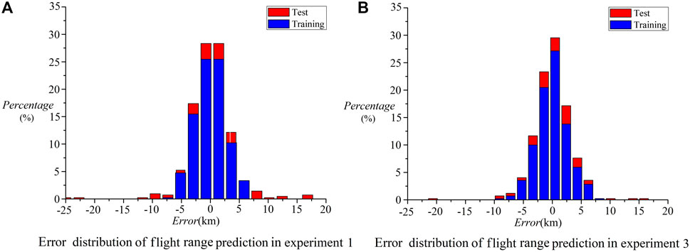
FIGURE 7. Range $R_D$ prediction results.

FIGURE 8

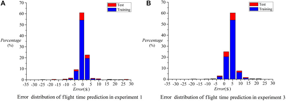
FIGURE 8. Flight time $T_D$ prediction results.

The random state test is carried out for the established prediction model. Table 3 shows the range and flight time calculated by using neural network and trajectory model, respectively, under the randomly selected 10 groups of parameter combinations. From the comparison of results, the maximum error between the range prediction value R_D(BP) and the trajectory calculation value R_D(Tra) is in condition 4. The relative error of the two algorithms is less than 0.82%, and the error of other conditions is less than 0.3%. The maximum relative error between the predicted value T_D(BP) of flight time and the calculated value T_D(Tra) of trajectory is within 0.45%. It can be seen that the neural network prediction model has high accuracy.

TABLE 3

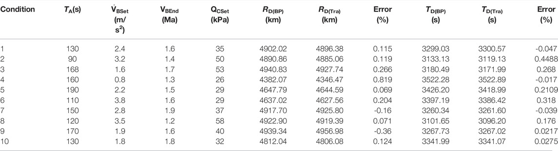
TABLE 3. Range and flight time prediction results.

5.2 Parameter Optimization

The aircraft’s range is an important indicator of the overall design. In the trajectory design, overload, attack angle, dynamic pressure, etc. have been reflected in the flight model as constraints, so the range $R_D$ is used as the objective function of trajectory optimization.

A genetic algorithm is used to optimize the overall parameters of the established neural network prediction model. The main parameters of the algorithm refer to the values in the study by Cheng and Wang (2011), and the settings are listed in Table 4:

TABLE 4

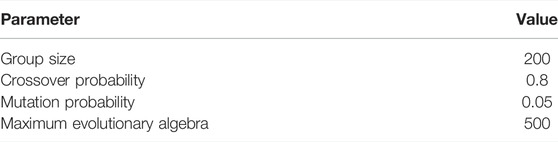
TABLE 4. Main parameters of genetic algorithm.

In order to test the influence of genetic algorithm parameters, the group sizes of 50, 100, 150, 200, and 250 are taken, and the optimal value of R_D obtained by optimization varies from 4991.40 to 4992.26 km; Take five groups of mutation probability of 0.05, 0.10, 0.15, 0.20, and 0.25. The variation range of R_D is 4991.40–4992.78 km, and its relative variation value is very small. For the training model, the change of algorithm parameters is not sensitive to the optimization results, so it can be carried out according to the parameter values in Table 4.

Based on the parameter settings in Table 4, a total of 138 steps are iterated, and the calculated results are listed in Table 5. From the optimization results, the flight pressure is close to 40 kPa, which is similar to the ballistic characteristics analysis results in Section 4.

TABLE 5

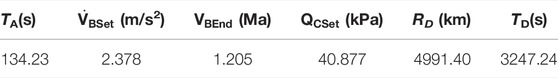
TABLE 5. Optimization calculation results.

The optimal value in Table 5 is used as the input parameter for trajectory calculation. Under this condition, the flight time of the aircraft is 3247.60 s and the range is 4981.15 km. The result of the trajectory calculation is basically consistent with the time prediction value in Table 4. The range value is slightly smaller, and the relative error is 0.2058%. Comparing the overall parameters of the sample points, the optimized results, and the optimal point of trajectory calculation in Figure 9, it can be seen that the optimized result range $R_D$ is the best, and the flight time $T_D$ is at the middle level of the sample points.

FIGURE 9

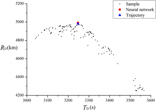
FIGURE 9. Comparison between optimization results and sample points.

The trajectory and parameter changes in the optimized state are shown in Figure 10. From the analysis of the flight process, since the end speed of Section 2 is Ma1.205, the proportion of this section in the climb process is relatively small, and it is transferred to Section 3 isodynamic flight when the flight altitude is about 8.7 km. During the whole climbing process, the flight speed continued to increase, and the acceleration in the isodynamic pressure section was large. After the change of dynamic pressure, the maximum value is about 55 kPa, which does not exceed the upper and lower limits of constraints, and the parameter changes are within a reasonable range.

FIGURE 10

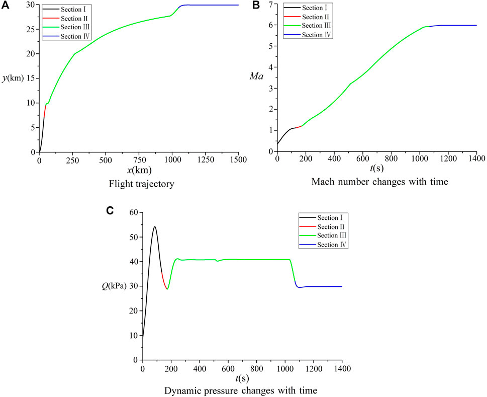
FIGURE 10. Parameter variation of the optimized trajectory.

6 Conclusions

In this paper, research on the parametric modeling of the trajectory is carried out for hypersonic vehicles. Based on the calculation results of the sample points, a neural network model for predicting the flight range and flight time is established, and the genetic algorithm is used to optimize the flight range prediction model. The research has the following conclusions:

(1) The flight process of hypersonic aircraft is complex, and the parameters between each section are mutually constrained. Parametric modeling can be achieved, by designing the flight process as a combination of typical sections and extracting the parameters that affect the sections.

(2) From the influence of typical parameters, the flight dynamic pressure $Q_{CSet}$ is more sensitive to the parameters of the climbing section and the range of the aircraft. When the dynamic pressure is lower than 30 kPa, the climb time will be significantly increased, the fuel will be consumed, and the range will be significantly reduced; when the dynamic pressure is higher than 50 kPa, the range will also decrease.

(3) Based on the sample points, a BP neural network for predicting the range and flight time was established, and the random state test was used. The errors of the range R_D and flight time T_D, relative to the calculation results of the trajectory model were within 0.82% and 0.45%, respectively, indicating that the established model has good prediction ability for overall parameter value of the aircraft trajectory.

(4) The genetic algorithm is used to optimize the prediction model, and the error of R_D between the optimization point and the trajectory calculation result is about 0.2% with the maximum range as the objective function. The flight process in the optimized state has a good balance between the flight range and the flight time.

By parametric modeling of the flight section of the hypersonic vehicle and optimization based on the range prediction model, the optimization of the complex flight process can be realized, and it is easy to extend to the modeling process of more parameters and section combinations.

Data Availability Statement

The original contributions presented in the study are included in the article/Supplementary Material, further inquiries can be directed to the corresponding author.

Author Contributions

In this article, FC establishes the trajectory calculation model and the neural network model for parameter prediction and carries out the trajectory optimization calculation and analysis. XH completed the calculation and characteristic analysis of the sample trajectory.

Conflict of Interest

The authors declare that the research was conducted in the absence of any commercial or financial relationships that could be construed as a potential conflict of interest.

Publisher’s Note

All claims expressed in this article are solely those of the authors and do not necessarily represent those of their affiliated organizations, or those of the publisher, the editors, and the reviewers. Any product that may be evaluated in this article, or claim that may be made by its manufacturer, is not guaranteed or endorsed by the publisher.

References

Ahuja, V., and Hartfield, R. J. (2015). Optimization of Scramjet Combustor Geometries Using Genetic Algorithms. J. Propulsion Power 31 (5), 1481–1485. doi:10.2514/1.b35397

CrossRef Full Text | Google Scholar

Antunes, A. P., and Azevedo, J. L. F. (2014). Studies in Aerodynamic Optimization Based on Genetic Algorithms. J. Aircraft 51 (3), 1002–1012. doi:10.2514/1.c032095

CrossRef Full Text | Google Scholar

Benson, D. A., Huntington, G. T., Thorvaldsen, T. P., and Rao, A. V. (2006). Direct Trajectory Optimization and Costate Estimation via an Orthogonal Collocation Method. J. Guidance, Control Dyn. 29 (6), 1435–1440. doi:10.2514/1.20478

CrossRef Full Text | Google Scholar

Cheng, J. N., and Wang, H. P. (2011). Hybrid Genetic Algorithm Global Optimization of Configuration Design for Ballistic Missiles. Flight Dynamic 29 (3), 44–47. doi:10.13645/j.cnki.f.d.2011.03.023

CrossRef Full Text | Google Scholar

Cui, N. G., Guo, D. Z., and Li, K. Y. (2020). A Survey of Numerical Methods for Aircraft Trajectory Optimization. Tactical Missile Tech. 5, 37–51. doi:10.16358/j.issn.1009-1300.2020.1.536

CrossRef Full Text | Google Scholar

Darby, C. L., Hager, W. W., and Rao, A. V. (2011). Direct Trajectory Optimization Using a Variable Low-Order Adaptive Pseudospectral Method. J. Spacecraft Rockets 48 (3), 433–445. doi:10.2514/1.52136

CrossRef Full Text | Google Scholar

Gandhi, M., and Theodorou, E. (2016). “A Comparison between Trajectory Optimization Methods: Differential Dynamic Programming and Pseudospectral Optimal Control,” in Proceeding of the AIAA Guidance, Navigation, and Control Conference, San Diego, California, USA, January 2016. doi:10.2514/6.2016-0385

CrossRef Full Text | Google Scholar

Gath, P., and Calise, A. (1999). Optimization of Launch Vehicle Ascent Trajectories with Path Constraints and Coast Arcs. J. Guidance, Control Dyn. 24, 296–304. doi:10.2514/6.1999-4308

CrossRef Full Text | Google Scholar

Jia, X. J., and Yan, X, D. (2015). Ascent Trajectory Design Method for Air-Breathing Powered Propulsion System. J. Northwest. Polytechnical Univ. 33 (1), 104–109. doi:10.3969/j.issn.1000-2758.2015.01.022

CrossRef Full Text | Google Scholar

Li, Y. I., Tong, H., Song, G., and Dong, L. I. (2006). Application of Neural Network in Calculation of Aircraft’s Flight Track Simulation. J. Naval Aeronaut. Eng. Inst. 21 (5), 541–544. doi:10.3969/j.issn.1673-1522.2006.05.012

CrossRef Full Text | Google Scholar

Li, X., Liu, C. A., Wang, Z. J., and Zhang, H. J. (2012). Trajectory Optimization for Maximizing Cruise Range of Air-Breathing Hypersonic Missile. Acta Armamentarii 33 (3), 290–294.

Google Scholar

Liu, R. F., Yu, Y. F., and Yan, B. B. (2016). Ascent Phase Trajectory Optimization for Hypersonic Vehicle Based on Hp-Adaptive Pseudospectral Method. J. Northwest. Polytechnical Univ. 34 (5), 790–797. doi:10.3969/j.issn.1000-2758.2016.05.008

CrossRef Full Text | Google Scholar

Liu, X. (2017). Research on Trajectory Optimization and Guidance for Hypersonic Cruise Vehicles. Wuhan: Huazhong University of Science and Technology.

Google Scholar

Lu, X., He, G. Q., and Liu, P. J. (2010). Ascent Trajectory Design Method for RBCC-Powered Vehicle. Acta Aeronautica Et Astronautica Sinica 31 (7), 1331–1337.

Google Scholar

Ma, T. R., Sheng, Y. Z., and Zhang, X. P. (2020). “The Trajectory Generation via Deep Neural Network for Hypersonic Vehicle,” in Proceeding of the 9th International Symposium on Computational Intelligence and Industrial Applications (ISCIIA2020), Beijing, China, Oct.31-Nov.3.

Google Scholar

Mei, Y. X., Feng, Y., Wang, R. S., Wu, L. N., and Sun, H. F. (2019). Fast Optimization of Reentry Trajectory for Hypersonic Vehicles with Multiple Constraints. J. Astronautics 40 (7), 758–767. doi:10.3873/j.issn.1000-1328.2019.07.004

CrossRef Full Text | Google Scholar

Narayanaswamy, S., and Damaren, C. J. (2020). Comparison of the Legendre-Gauss Pseudospectral and Hermite-Legendre-Gauss-Lobatto Methods for Low-Thrust Spacecraft Trajectory Optimization. Aerospace Syst. 3, 53–70. doi:10.1007/s42401-019-00042-w

CrossRef Full Text | Google Scholar

Oktay, T., Arik, S., Turkmen, I., Uzun, M., and Celik, H. (2018). Neural Network Based Redesign of Morphing UAV for Simultaneous Improvement of Roll Stability and Maximum Lift/drag Ratio. Aircraft Eng. Aerospace Tech. 90, 1203–1212. doi:10.1108/aeat-06-2017-0157

CrossRef Full Text | Google Scholar

Olds, J., and Budianto, I. (1998). “Constant Dynamic Pressure Trajectory Simulation with POST,” in Proceeding of the 36th AIAA Aerospace Sciences Meeting and Exhibit, Reno,NV,U.S.A., January 1998. doi:10.2514/6.1998-302

CrossRef Full Text | Google Scholar

Patrón, R. S. F., and Botez, R. M. (2015). Flight Trajectory Optimization through Genetic Algorithms for Lateral and Vertical Integrated Navigation. J. Aerospace Inf. Syst. 12 (8), 533–544. doi:10.2514/1.i010348

CrossRef Full Text | Google Scholar

Qian, S. Y. (2021). Trajectory Planning and Reentry Guidance for Boost-Glide Vehicle. Harbin: Harbin Institute of Technology.

Google Scholar

Reddien, G. W. (1979). Collocation at Gauss Points as a Discretization in Optimal Control. SIAM J. Control. Optim. 17 (2), 298–306. doi:10.1137/0317023

CrossRef Full Text | Google Scholar

Tang, X. J., Li, Z. T., and Zhang, H. B. (2021). Ascent Guidance Method for Combined-Cycle Vehicle Based onReceding Horizon Pseudo-spectral Optimization. J. Ballistics 33 (4), 1–8. doi:10.12115/j.issn.1004-499X(2021)04-001

CrossRef Full Text | Google Scholar

Tao, C. (2017). Trajectory Optimization and Tracking Controller Based on Gauss Pseudo Spectral Method for Hypersonic Vehicle. J. Syst. Simulation 29 (4), 865∼872+879. doi:10.16182/j.issn1004731x.joss.201704022

CrossRef Full Text | Google Scholar

Wang, T. S., Sun, Z. G., Huang, Z., and Xi, G. (2021). Reconstruction of Fluid Flows Past Airfoils Using Neural Network. J. Eng. Thermophys. 42 (5), 1205–1212.

Google Scholar

Wei, Y. Y. (2022). Major Technological Issues of Aerospace Vehicle with Combined-Cycle Propulsion. Aerospace Tech. 1, 1–12. doi:10.16338/j.issn.2097-0714.20220601

CrossRef Full Text | Google Scholar

Xie, Y., Franz, E., Chu, M., and Thuerey, N. (2018). TempoGAN: A Temporally Coherent, Volumetric GAN for Super-resolution Fluid Flow. ACM Trans. Graphics 37 (4), 951–9515. doi:10.1145/3197517.3201304

CrossRef Full Text | Google Scholar

Zhang, D. Q., Song, W. T., Chai, Z., Liu, L. L., and Meng, P. P. (2014). Aircraft/engine Performance Integrate Analysis on Combined Cycle Engine. J. Aerospace Power 32 (10), 2498–2507. doi:10.13224/j.cnki.jasp.2017.10.024

CrossRef Full Text | Google Scholar

Zhang, T. (2013). Research on Trajectory Optimization of Air-Breathing Hypersonic Vehicle. Harbin: Harbin Institute of Technology.

Google Scholar

Zhang, W. D. (2017). Reentry Trajectory Planning and Attitude Control for Hypersonic Glide Vehicles. Harbin: Harbin Institute of Technology.

Google Scholar

Zhang, X., and Li, G. R. (2020). Prediction Model of Ship Trajectory Based on GA-BP. J. Guangzhou Maritime Univ. 28 (4), 15–18.

Google Scholar

Zhao, J., and Zhou, R. (2013). Reentry Trajectory Optimization for Hypersonic Vehicle Satisfying Complex Constraints. Chin. J. Aeronautics 26 (6), 1544–1553. doi:10.1016/j.cja.2013.10.009

CrossRef Full Text | Google Scholar

Zheng, X., Liu, Z. S., Yong, Y., Lei, J. C., and Li, Z. X. (2018). Research on Climb-Cruise Global Trajectory Optimization for RBCC Hypersonic Vehicle. Missiles and Space Vehicles 2, 1–8. doi:10.7654/j.issn.1004-7182.20180201

CrossRef Full Text | Google Scholar

Zheng, T. Y., Yao, Y., and He, F. H. (2020). Trajectory Estimation of a Hypersonic Flight Vehicle via L-EKF. J. Harbin Inst. Tech. 52 (6), 160–170. doi:10.11918/202003094

CrossRef Full Text | Google Scholar

Zhou, H. Y., Wang, X. G., Zhao, Y. L., and Cui, N. (2020). Ascent Trajectory Optimization for a Multi-Combined-Cycle-Based Launch Vehicle Using a Hybrid Heuristic Algorithm. J. Astronautics 40 (1), 61–70. doi:10.3873/j.issn.1000-1328.2020.01.008

CrossRef Full Text | Google Scholar

Zhu, R. Y., Qi, Z., Wang, L. S., Miao, M., Bai, G. H., Wang, C., et al. (2020). Trajectory Optimization Design of Morphing Vehicle. Tactical Missile Tech. 5, 157–164. doi:10.16358/j.issn.1009-1300.2020.1.085

CrossRef Full Text | Google Scholar