Multi-Objective Optimal Source–Load Interaction Scheduling of Combined Heat and Power Microgrid Considering Stable Supply and Demand

1 Introduction

Combined heat and power microgrid (CHP-MG) based on the concept of multi-energy complementation, energy cascade utilization, and the coordination and optimization of multi-type heterogeneous energy subsystems breaks the mode of discrete planning and operation between energy systems and effectively improves the utilization rate of energy (Alomoush, 2019; Blair and Mabee, 2020; Nojavan et al., 2020; Hemmati et al., 2021a; Wang et al., 2021a). In recent years, many scholars have done many pioneering research studies on the modeling and optimal scheduling of the source and load sides of the CHP-MG system (Freeman et al., 2017; Ippolito and Venturini, 2018; Zhao et al., 2019; Ronaszegi et al., 2020; Singh and Kumar, 2020; Jordehi, 2021).

On the source side, Pashaei-Didani et al. (2019) proposed a fuel cell system including a reformer, a hydrogen storage tank, and a fuel cell using natural gas as a raw material. At the same time, the heat production characteristics of hydrogen production from natural gas reforming and the thermoelectric hydrogen coupling characteristics of fuel cells were considered, which effectively reduced the microscopic grid emissions and costs. Hemmati et al. (2021b) improved system operation/recovery and reduced operation/energy costs by optimizing CHP size, location, and equipment operation. In the above research, the optimization target only considers the economic cost and environmental cost and lacks the consideration of the supply-side stability of the system. For example, frequent switching of the start-up state of the equipment or relatively large adjustment of the operating power not only affects the stability and service life of the equipment but also increases the complexity of the transportation, storage, and scheduling of natural gas and other fuels. For source-side optimization scheduling, Liu and Yang (2022) propose a primal–dual based dynamic weight distributed algorithm for multi-objective optimal scheduling of distributed integrated energy system, so as to reduce the operating cost and environmental cost of the system. It is proved that the algorithm has better flexibility, reliability, and adaptability and lower communication burden. Yi et al. (2020) proposed a distributed, neurodynamic-based approach for economic dispatch in an integrated energy system. Compared with other centralized and distributed optimization methods, it is shown that the proposed distributed optimization method has advantages in convergence speed and computational complexity. Anh and Cao (2020) proposed an optimal energy management (OEM) approach that uses smart optimization techniques to achieve optimal hybrid thermoelectric isolation microgrids. Naderipour et al. (2020) proposed the use of particle swarm optimization algorithm to optimize the configuration of the cogeneration system to reduce the operating cost on the basis of considering the maximum allowable capacity. It can be seen that the centralized algorithm is mostly used in a single energy system. For distributed large-scale energy systems, the distributed algorithm has better solving ability than the centralized algorithm.

For the load side, flexible electrical and thermal loads can also be used as potential targets for optimal scheduling of CHP-MG systems. How to quantify and guide the flexible load to participate in each link of the optimal operation of the system and promote the good interaction between source and load has gradually become a research hotspot (Liu et al., 2018; Mohseni et al., 2021; Zhou, 2019; Dranka et al., 2021; Hca et al., 2021; Jiang et al., 2021; Amir et al., 2019)

Integrated demand response should adopt price, policy, contract, and other methods to guide users to change their energy consumption habits and optimize the source–load matching relationship of the energy system, so we can obtain greater comprehensive benefits (Aghamohammadloo et al., 2021; Li et al., 2021a; Salehimaleh et al., 2022; Zhang et al., 2019). Lv et al. (2021) have built an IDR multi-time scale optimal scheduling model for power, gas, and heat loads. Zhang et al. (2015) proposed to use a piecewise linear function to characterize the cost of reducing the load and determine the IDR price according to the marginal cost corresponding to various energy consumption in a specific period. Munoz-Delgado et al. (2016) adopted the method of stochastic programming and generated a large number of discrete scenes based on the scene method to represent the uncertainty of DG output and load and convert the uncertainty problem into a deterministic problem. Shao et al. (2020) by incorporating the demand-side response of the energy hub into the integrated power and natural gas system solved the problem that the complex coupling relationship between power and natural gas may reduce the flexibility of system operation. Wc et al. (2021) proposed an optimization technique based on integrated demand response and tolerance of household energy management.

Most of the above studies focus on user load while ignoring the benign interaction between source and load. Load reduction and transfer will greatly affect user satisfaction with energy consumption. However, the conversion and substitution of heating forms (electric heating/gas heating) on the side of the load has little influence on the user’s energy experience. And there are few studies to establish a comprehensive evaluation system that considers both the supply and the demand of users. In addition, most of them only focus on user load, ignoring the benign interaction between source and load. For example, renewable energy on the supply side has great volatility and randomness (Yang et al., 2018; Salama et al., 2021), and the negative impact of this factor can be alleviated through IDR. Li et al. (2019) introduced the interaction between energy supplier and customer into system model development. On this basis, considering the characteristics of different time scales of electricity and heat, an event-triggered distributed algorithm is used to optimize scheduling, smoothing real-time load changes and renewable resource fluctuations while maximizing day-ahead social welfare.

To sum up, this paper proposes a multi-objective coordinated optimal scheduling method for cogeneration microgrid source–load that considers the stability of supply and demand. Compared with the existing research, the difficulties and challenges as well as the innovations and contributions made in this paper are as follows:

1) The existing studies on the source side mostly consider economy and environmental protection but lack the consideration of supply stability. In this paper, the CHP-MG model makes use of energy storage equipment to decouple thermoelectric connection and expand the power supply capacity through multi-energy devices. Meanwhile, the supply stability is taken as one of the criteria to evaluate the operation.

2) For the demand response of the load side, most of them adopt the method of load reduction and transfer, which will greatly affect the user’s energy satisfaction. Therefore, in addition to the construction of a comprehensive demand response model that includes the electrical load that can be time-shifted and interrupted, electrical loads that can be time-shifted and uninterrupted, the curtailable electrical load, the curtailable heat load, it also considers the integrated demand response model for heat supply mode conversion and introduces a flexible IDR price compensation mechanism. In addition, a comprehensive satisfaction evaluation system was established considering the demand-side user energy deviation degree, IDR compensation price, supply-side heating and power supply flexibility, and other factors.

3) For the problem that most IDR only focuses on user load but ignores the benign interaction between source and load, the fluctuation of renewable energy is smoothed by the IDR of load side.

4) The solution of CHP-MG model has the characteristics of high dimensionality and non-linearity, so an intelligent algorithm is needed to approximate the optimal solution. In addition, compared with the distributed large-scale energy system, the system is of single cogeneration type, and the amount of information and calculation is small, so the centralized optimization algorithm is adopted. In this paper, the improved multi-objective grey wolf optimizer (MOGWO) is used to carry out the source–charge interaction multi-objective optimal scheduling of microgrids, and through example analysis, it is verified that the algorithm can promote the benign interaction between source and load and ensure the stability of supply and demand (SDS) and economy of CHP-MG operation.

2 General Framework of the System

The system is roughly divided into two parts, the source side and the load side, and its framework is shown in Figure 1.

FIGURE 1

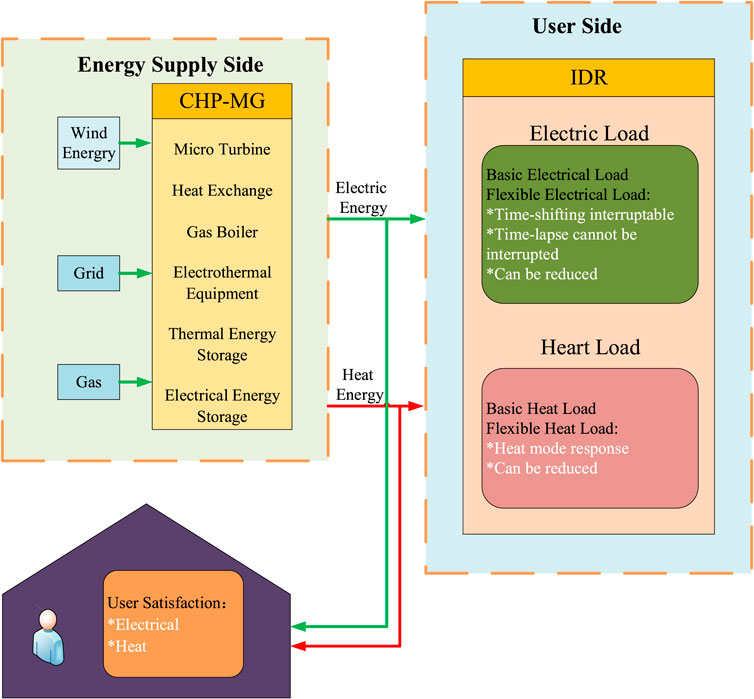
FIGURE 1. System overall framework diagram.

The source side contains wind energy and CHP-MG systems, which use wind energy, electric energy, and natural gas as sources to provide customers with both electric and thermal energy through the complementary use of multiple energy sources.

In the CHP-MG system, the gas boiler consumes natural gas to generate heat, and the gas turbine consumes natural gas to generate electricity and at the same time generates a large amount of high-temperature flue gas, which is recovered by the heat exchanger to supply heat energy to the load side, thereby realizing the cascade utilization of energy. When the thermal energy generated by a gas turbine and gas boiler is greater than the demand of heating load, the excess thermal energy is stored in the thermal storage equipment. When the thermal energy produced is less than the heating load demand, the thermal energy storage device releases thermal energy. Electricity storage devices are similar to thermal storage devices.

The load side takes the residential load as the core, and the load is divided into two categories: electrical load and thermal load. The electrical load is divided into uncontrollable load and controllable load. Controllable load is further divided into time-shifted and interrupted, time-shifted and uninterrupted. The heat load is divided into the heat supply mode conversion load and the curtailable heat load. Among them, the heat load with convertible heating mode mainly considers the user’s behavior of abandoning the heating mode of electric heating and turning to the gas-heat mode of central heating due to the influence of price. The curtailable heat load mainly considers the flexible hot water load.

In order to ensure user experience and prevent the loss of customer groups, this paper establishes a user satisfaction evaluation system. When user satisfaction is lower than the warning value, the scheme should be abandoned. Among them, user satisfaction includes electricity consumption satisfaction and heat consumption satisfaction.

3 Source-Side Multi-Energy Complementary Model

In this paper, the CHP-MG contains three energy forms: heat, electricity, and gas. The system energy equipment mainly includes a wind turbine (WT), micro-turbine (MT), and gas boiler (GB); energy storage equipment includes electric energy storage (EES) and thermal energy storage (TES); energy conversion equipment includes heat exchanger (HE) and electrothermal equipment (EE). Its structure is shown in Figure 2. This system has energy interaction with the external power grid (PG).

FIGURE 2

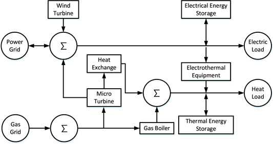
FIGURE 2. CHP-MG source-side system structure diagram.

3.1 Wind Turbine

The research shows that the output power of wind turbine ($P_w$) depends on the wind speed and the rated output power of wind turbine ($P_r$). In addition, the wind speed obeys Weibull distribution. Therefore, the probability density function (PDF) of $P_w$ can be expressed as

$f_w\left(P_w\right)=\{\begin{array}{c}\left(kh{v}_{in}/\epsilon P_r\right)\times \\ {\left[\left(\left(1+h{P}_w/P_r\right)v_{in}\right)/\epsilon \right]}^{k-1}\times \\ exp\left\{-{\left[\left(\left(1+h{P}_w/P_r\right)v_{in}\right)/\epsilon \right]}^k\right\},\\ P_w\in \left[0,P_r\right]\\ 0,otherwise\end{array}(1)$

Here, $\epsilon$ is the scaling factor; $k$ is the shape factor, reflecting the average wind speed or the average output power of the wind turbine in a certain period; and $h=\left(v_r/v_{in}\right)-1$, in which $v_{in}$ and $v_r$ are the cut-in and rated wind speeds, respectively. More details of the probabilistic WT model can be found in the study of Yang et al. (2019).

In order to reduce the influence of uncertain wind power on system scheduling, this paper takes the mathematical expectation $P_{WT}^t$ of $P_w$ at each time period as the reference value (Li et al., 2021b).

3.2 Micro-Turbine

This paper focuses on the heat and power supply of MT, ignoring the effect of environmental changes on power generation and combustion efficiency. Its heat generation power $Q_{MT}^t$ is

$Q_{MT}^t=P_{MT}^t\frac{\left(1-{\eta }_{MT}-{\eta }_L\right)}{{\eta }_{MT}}.(2)$

Here, $P_{MT}^t$ is the electric generation power of MT in period t and ${\eta }_{MT}$, ${\eta }_L$ are the power generation efficiency and heat loss coefficient of MT.

Operating power constraints and climbing constraints are

$\{\begin{array}{c}{I}_{MT}^t{P}_{MT,\min }\le P_{MT}^t\le I_{MT}^t{P}_{MT,\max },\\ d{P}_{MT,\min }\le P_{MT}^t-P_{MT}^{t-1}\le d{P}_{MT,\max }\end{array}(3)$

Here, $P_{MT,\text{max}}$/$P_{MT,\text{min}}$ and $d{P}_{MT,\text{max}}$/$d{P}_{MT,\text{min}}$ are the upper and lower limits of MT operating power and climbing rate and $I_{MT}^t$ is the status flag bit of MT, which is 1 when running and 0 when stopped.

3.3 Heat Exchanger

The waste heat discharged from the MT is converted into usable heat energy by the HE:

$Q_{HE}^t=Q_{MT}^t{\eta }_{MT}(4)$

Here, $Q_{HE}^t$ is the heat production power of HE in period t and ${\eta }_{MT}$ is the thermal efficiency of HE.

3.4 Gas Boiler

The GB generates heat energy by consuming natural gas to supplement the heat load when HE and TES are insufficient. The relationship between output power and input power is

$\{\begin{array}{c}{Q}_{GB,\min }\le Q_{GB}^t\le Q_{GB,\max }\\ d{Q}_{GB,\min }\le Q_{GB}^t-Q_{GB}^{t-1}\le d{Q}_{GB,\max }\end{array}(5)$

Here, $Q_{GB,\text{max}}$/$Q_{GB,\text{min}}$ and $d{Q}_{GB,\text{max}}$/$d{Q}_{GB,\text{min}}$ are the upper and lower limits of GB operating power and climbing rate.

3.5 Electrothermal Equipment

Electrothermal equipment consumes electric energy for heat production, such as air conditioners and electric boilers. The relationship that needs to be satisfied is

$\{\begin{array}{c}{Q}_{EE}^t=Q_{EE}^t{\eta }_{EE}\\ Q_{EE,\min }\le Q_{EE}^t\le Q_{EE,\max }\end{array}(6)$

Here, $Q_{EE}^t$ is the heat generation power of EE in period t; ${\eta }_{EE}$ is the thermal efficiency of EE; and $Q_{EE,\text{max}}$, $Q_{EE,\text{min}}$ are the upper and lower limits of EE heat generation power.

3.6 Energy Storage Equipment

In this paper, the energy storage device is mainly used to decouple the complex electrical and thermal connection, so that the CHP-MG system can get rid of the traditional mode of “determining electricity by heat” and “determining heat by electricity.” On this basis, the system runs in the direction of supply and demand stability and optimal economy.

3.6.1 Electricity Storage Equipment

EES is often used in microgrids to achieve peak-shaving and valley-filling of electrical loads, smooth operation of generation equipment, and reduction of operating costs. The relationship between power and energy storage capacity during the operation of EES is shown below.

Energy storage constraint:

$\{\begin{array}{c}\begin{array}{c}{E}_{EES}^t=E_{EES}^{t-1}+\left(P_{EES,c}^t{\eta }_c-\frac{P_{EES,d}^t}{{\eta }_d}\right)\\ E_{EES,\min }\le E_{EES}^t\le E_{EES,\max },\end{array}\\ E_{EES}^0=E_{EES}^{24}.\end{array}(7)$

Here, $E_{EES}^t$ is the storage capacity of EES in period t; $P_{EES,c}^{t-1}$ is the charging power of EES in period t-1; $P_{EES,d}^t$ is the discharge power of EES in period t; ${\eta }_c$/${\eta }_d$ is the charge/discharge coefficient of EES; and $E_{EES,\text{max}}$/$E_{EES,\text{min}}$ is the maximum/minimum capacity of EES.

Power constraint:

$\{\begin{array}{c}{P}_{EES,c,\min }{I}_{EES,c}\le P_{EES,c}^t\\ \le P_{EES,c,\max }{I}_{EES,c}\\ P_{EES,d,\min }{I}_{EES,d}\le P_{EES,d}^t\\ \le P_{EES,d,\max }{I}_{EES,d}\end{array}(8)$

Here, $P_{EES,c,\text{max}}$/$P_{EES,c,\text{min}}$ is the maximum/minimum charging power of EES; $P_{EES,d,\text{max}}$/$P_{EES,d,\text{min}}$ is the maximum/minimum discharge power of EES; and $I_{EES,c}$/$I_{EES,d}$ is the charge/discharge status flag of EES, which is 0 when stopped and 1 when running. The mutual exclusion constraint needs to be satisfied, that is,

$I_{EES,c}+I_{EES,d}\le 1(9)$

$\{\begin{array}{c}d{P}_{EES,c,\min }\le P_{EES,c}^t-P_{EES,c}^{t-1}\\ \le d{P}_{EES,c,\max }\\ d{P}_{EES,d,\min }\le P_{EES,d}^t-P_{EES,d}^{t-1}\\ \le d{P}_{EES,d,\max }\end{array}(10)$

Here, $d{P}_{EES,c,\text{max}}$/$d{P}_{EES,c,\text{min}}$ is the maximum/minimum ramp rate for charging EES and $d{P}_{EES,d,\text{max}}$/$d{P}_{EES,d,\text{min}}$ is the maximum/minimum ramp rate of EES discharge.

3.6.2 Heat Storage Equipment

An energy storage device is a storage device for energy, not just for electrical energy. Generally, the peak of electricity consumption occurs during the day, and the peak of heat consumption occurs in the morning and evening, resulting in a mismatch between the electric heat output and the electricity load. Therefore, TES is used in this paper to realize the translation of heat time and solve the difference in the time of electric–thermal load. In order to simplify the model, without considering the influence of environmental factors on heat self-loss rate, the TES constraint relationship is similar to that of EES, as shown below.

Energy storage constraint:

$\{\begin{array}{c}{E}_{TES}^t=\left(1-\delta \right)E_{TES}^{t-1}+\\ \left(Q_{TES,c}^t{\delta }_c-\frac{Q_{TES,d}^t}{{\delta }_d}\right)\\ E_{TES,\min }\le E_{TES}^t\le E_{TES,\max }\end{array}(11)$

Here, $E_{TES}^t$ is the heat storage of TES in period t; $Q_{TES,c}^{t-1}$ is the heat storage of EES in period t-1; $Q_{TES,d}^t$ is the exothermic power of TES in period t; ${\delta }_c$/${\delta }_d$ is the heat storage/release coefficient of TES; $\delta$ is the self-loss coefficient of TES; and $E_{TES,\text{max}}$/$E_{TES,\text{min}}$ is the maximum/minimum capacity of TES.

The power constraint and climbing constraint satisfied by TES are consistent with those of EES and will not be discussed in this paper.

4 Comprehensive Demand Response Model of Load Side

The IDR behavior of users on the load side of the CHP-MG system is divided into the response of electric load demand and the response of thermal load demand. It is assumed that the user’s IDR mode adopts the following strategies:

1) In the case of satisfying user satisfaction, the thermal load can be flexibly responded by adjusting the demand of electric/gas heat load and the reduction of heat load.

2) In the case of satisfying user satisfaction, the electrical load can be flexibly responded by shifting and interrupting and reducing the electrical load.

Among them, the flexible electrical loads, that is, electrical loads that participate in response, can be divided into the time-shiftable and interruptible electric load, the time-shiftable non-interruptible load, and the curtailable electric load. Flexible heat loads, that is, the heat loads that participate in response, are reducible heat loads. In addition, for flexible heat load, this paper considers the user’s choice of heating mode.

4.1 Flexible Electrical Load

4.1.1 Time-Shiftable and Interruptible Load

Time-shiftable and interruptible load means that the load’s power consumption time can be shifted and interrupted according to system requirements. The working duration and the number of interruptions of different electrical appliances are different. Assuming that the number of devices participating in demand response is $n_{b,int}$, the charging time of device $n$ is $T_{b,n}$, the number of interrupts is $q_{b,n}$, and the transferable range is $\left[t_{b,n,s},t_{b,n,e}\right]$, the following relationship must be satisfied:

$\{\begin{array}{c}{q}_{b,n}\le q_{b,n,\max },\\ U_b=\left[t_{b,n,s1},t_{b,n,e1}\right]\cup \left[t_{b,n,s2},t_{b,n,e2}\right]\\ \cdots \cup \left[t_{b,n,s\left(q_{b,n}+1\right)},t_{b,n,e\left(q_{b,n}+1\right)}\right].\end{array}(12)$

Here, $q_{b,n,\text{max}}$ is the maximum number of interruptions of device $n$; $t_{b,n,si}$/$t_{b,n,ei}$ is the actual time point of the ith start/end of device n; and $U_b$ is the set of working time periods after the device n is shifted and interrupted.

The electric load $L_{b0}^t$/$L_b^t$ expression before/after the translation and interruption is

$\{\begin{array}{c}{L}_{b0}^t={\displaystyle \sum _{n=1}^{n_{b,\mathrm{int}}}{L}_{b0,n}^t}\\ L_b^t={\displaystyle \sum _{n=1}^{n_{b,\mathrm{int}}}{L}_{b,n}^t}\\ L_{b0,n}^t=\{\begin{array}{cc}0& t\notin \left[t_{b,n,s0},t_{b,n,e0}\right]\\ P_{b,n}& t\in \left[t_{b,n,s0},t_{b,n,e0}\right]\end{array}\\ L_{b,n}^t=\{\begin{array}{cc}0& t\notin U_b\\ P_{b,n}& t\in U_b\end{array}\end{array}(13)$

Here, $P_{b,n}$ is the rated power of the device n; $L_{b0,n}^t$ is the ideal response of equipment n to the electrical load demand in time period t; and $L_{b,n}^t$ is the response electrical load demand of device n after time shift and interruption in time period t.

4.1.2 Time-Shiftable and Non-Interruptible Power Loads

Time-shiftable and non-interruptible power load means that the load’s power consumption time can be shifted according to system requirements, and the working duration of different electrical appliances is different. The modeling process of the electrical loads $L_{a0}^t$, $L_a^t$, etc., before/after translation is only a case when the number of interruptions in 4.1.1 is 0, so this section will not repeat them.

4.1.3 Electric Load Can Be Reduced

In the case of satisfying user satisfaction, the electric load can be appropriately reduced, and the electric load curve of the system load side can be smoothed. The correlation is as follows:

$\{\begin{array}{c}{L}_c^t=L_c^t-\Delta L_c^t,\\ \Delta L_c^t=I_{c,e}{\epsilon }_{c,e}^t{L}_{c0}^t,\\ {\epsilon }_{c,e,\min }\le {\epsilon }_{c,e}^t\le {\epsilon }_{c,e,\max }.\end{array}(14)$

Here, $\Delta L_c^t$ is the electrical load difference before/after reduction in period t; $L_c^t$ is the electrical load after reduction in time period t; $L_{c0}^t$ is the electric load participating in the reduction in time period t; ${\epsilon }_{c,e}^t$ is the electric load reduction coefficient after reduction in time period t; ${\epsilon }_{c,e,\text{max}}$/${\epsilon }_{c,e,\text{min}}$ is the maximum/minimum load reduction factor; and $I_{c,e}$ is the sign indicating whether the electric load is reduced, which is 1 when it is reduced.

4.2 Flexible Heat Load

4.2.1 Response of Heating Mode

The peak period of electrical loads such as air conditioners and electric furnaces is roughly the same as the peak period of grid power supply. Under the stimulation of price, some users gave up the heating method of electric heating and switched to the gas heating method of central heating. The relevant relationship is as follows:

$\{\begin{array}{c}\Delta H_a^t=I_{a,h}{\epsilon }_{a,h}^t{H}_{a0}^t,\\ D_a^t=\Delta H_a^t,\\ H_a^t=H_{a0}^t-D_a^t,\\ {\epsilon }_{a,h,\min }\le {\epsilon }_{a,h}^t\le {\epsilon }_{a,h,\max }.\end{array}(15)$

Here, $\Delta H_a^t$ is the heat load difference before/after the response by the heating method in the period t; $H_{a0}^t$ is the original gas heat load participating in the response of the heating mode in time period t; $H_a^t$/$D_a^t$ is the gas/electric heating load demand after the response of the heating mode in the period t; ${\epsilon }_{a,h}^t$ is the replacement coefficient in time period t; ${\epsilon }_{a,h,\text{max}}$/${\epsilon }_{a,h,\text{min}}$ is the maximum/minimum replacement coefficient; and $I_{a,h}$ is the sign indicating whether the heating mode response occurs to the heat load, which is 1 when the response occurs.

4.2.2 Reduced Heat Load

The main consideration of the heat load that can be reduced is the hot water load. Under the lowest water temperature $T_{w,\text{min}}$ acceptable by the user, appropriate reduction of the heat load can smooth the heat load curve on the load side of the system. The correlation is as follows:

$\{\begin{array}{c}{H}_{b,\min }^t=C_w{\rho }_w{v}_w^t\left(T_{w,\min }-T_{w,ini}\right),\\ H_{b0}^t=C_w{\rho }_w{v}_w^t\left(T_w^t-T_{w,ini}\right),\\ H_b^t=H_{b0}^t-\Delta H_b^t,\\ \Delta H_b^t=I_{b,h}{\epsilon }_{b,h}^t\left(H_{b0}^t-H_{b,\min }^t\right).\end{array}(16)$

Here, $C_w$, ${\rho }_w$ are the specific heat capacity and density of water; $v_w^t$ is the user’s hot water demand in time period t; $T_{w0}$ is the initial water temperature (15°C); $T_w^t$ is the ideal average temperature of hot water for the user in time period t; $H_{b,\text{min}}^t$ is the minimum hot water power required by the user in time period t; $\Delta H_b^t$ is the hot water load difference before/after the reduction in period t; $H_b^t$ is the hot water load reduced in time period t; $H_{b0}^t$ is the hot water load participating in the reduction in time period t; ${\epsilon }_{b,h}^t$ is the hot water load reduction coefficient in period t, whose value is between 0 and 1; and $I_{b,h}$ is a flag indicating whether the hot water load has been reduced, which is 1 when the reduction occurs.

4.3 IDR Price Compensation Mechanism

Price compensation encourages users to actively participate in demand response. Unlike the traditional fixed-ratio price compensation, this paper uses a flexible price compensation with the compensation cost $f_c$ shown as follows:

$f_c={\displaystyle \sum _{t=1}^{24}\left(\begin{array}{c}{\lambda }_{ab,e}^t{c}_{ab,e}^t\Delta L_a^t+\\ {\lambda }_{ab,e}^t{c}_{ab,e}^t\Delta L_b^t+\\ {\lambda }_{c,e}^t{c}_{c,e}^t\Delta L_c^t+\\ {\lambda }_{a,h}^t{c}_{a,h}^t\Delta H_a^t+\\ {\lambda }_{b,h}^t{c}_{b,h}^t\Delta H_b^t\end{array}\right)}.(17)$

Here, $c_{ab,e}^t$, $c_{c,e}^t$ are the unit compensation price for participating in time shift and interruption and reducing the response electric load in time period t; $c_{a,h}^t$, $c_{b,h}^t$ are the unit compensation price involved in adjusting the electric heating load and reducing the heat load response during period t; and ${\lambda }_{ab,e}^t$, ${\lambda }_{c,e}^t$, ${\lambda }_{a,h}^t$, and ${\lambda }_{b,h}^t$ are auxiliary variables with values between 0 and 1.

5 Source–Load Coordination and Interactive Optimization Scheduling

The optimal operation model of CHP-MG with IDR, decoupling the thermoelectric connection through the energy storage device, considering the multi-energy complementary characteristics, jointly formulates the optimal output plan of each coupling device from both sides of the source and the load, so as to improve the economy and supply and demand of the microgrid stability.

5.1 Objectives

5.1.1 Economics

When considering CHP-MG economy $F_1$, both the supply side and the demand side need to be considered. The energy supply cost $f_{CG}$ on the supply side includes the purchase cost of input energy and the aging cost of equipment, while the economy $f_{CD}$ on the demand side is mainly reflected in the compensation cost of users participating in IDR:

$\{\begin{array}{c}{F}_1=\min \left(f_{CG}+f_{CD}\right),\\ f_{CG}=f_{grid}+f_{EES}+\\ f_{TES}+f_{MT}+f_{GB}+f_{H_a},\\ f_{CD}=f_c.\end{array}(18)$

1) Large grid electricity purchase cost $f_{grid}$:

$f_{grid}={\displaystyle \sum _{t=1}^{24}{P}_{grid}^t{c}_{buy}^t}(19)$

Here, $P_{grid}^t$ and $c_{buy}^t$ are the purchase power and unit price of electricity from the microgrid to the large grid in time period t, respectively.

2) EES charge and discharge aging cost $f_{BT}$:

$f_{EES}={\displaystyle \sum _{t=1}^{24}{E}_{EES}^t{c}_{EES}^t}(20)$

Here, $c_{EES}^t$ is the unit aging price of EES in time period t.

3) TES charge and discharge aging cost $f_{BT}$:

$f_{TES}={\displaystyle \sum _{t=1}^{24}{E}_{TES}^t{c}_{BT}^t}(21)$

Here, $c_{TES}^t$ is the unit aging price of TES in time period t.

4) MT natural gas cost $f_{MT}$:

$f_{MT}={\displaystyle \sum _{t=1}^{24}{c}_{gas}^t}\frac{P_{MT}^t}{{\eta }_{MT}LH{V}_{gas}}.(22)$

Here, $c_{gas}^t$ is the price of natural gas in time period t and $LH{V}_{gas}$ is the low calorific value of natural gas, which is 9.7 kWh/m³.

5) GB natural gas cost $f_{GB}$:

$f_{GB}={\displaystyle \sum _{t=1}^{24}{c}_{gas}^t}\frac{Q_{GB}^t}{LH{V}_{gas}}(23)$

6) The cost of natural gas for electric heat to gas heat $f_{H_a}$ is

$f_{H_a}={\displaystyle \sum _{t=1}^{24}{c}_{gas}^t}\frac{H_{H_a}^t{\lambda }_{H_a}}{LH{V}_{gas}}(24)$

Here, ${\lambda }_{H_a}$ is the conversion factor of electricity–heat load.

5.1.2 Stability of Supply and Demand

While pursuing economy, CHP-MG system operators should also focus on providing a stable energy supply for users.

On the supply side, the stability of MT, GB, and external power grid is mainly considered. The stability of MT and GB output can reduce the frequent regulation of equipment, reduce the failure rate, and prolong the service life. In addition, as the main consumption equipment of natural gas, the MT and GB can also improve the input stability of natural gas and reduce the complexity of transportation and management. Keeping the power interaction with the external grid stable improves the stability and safety of the system while reducing the stress caused by the CHP-MG system to the outside.

On the demand side, it mainly measures the discrete degree of the difference between the user’s electricity load and the wind power load (LW). Because wind power load is easily affected by environmental factors, its load curve is highly discrete, which increases the difficulty in hardware and software regulation of microgrid. The traditional load prediction curve is usually “peak-cutting and valley-filling” by an energy storage device, but the load prediction curve often represents a larger possible state of wind turbine output while ignoring other output possibilities. In this paper, the mathematical expectation $P_{WT}^t$ of $P_w$ in time period t is taken as the “equilibrium point” of output possibility of wind turbine in time period t, so that the optimized operation process of the system works near the “equilibrium point” of wind turbine. In addition, the CHP-MG system adjusts the electrical load curve through IDR and smoothes the difference curve between user power load and wind power load.

In this paper, the weighted value of the change rate of the output curve of each load or equipment is used to evaluate the supply and demand stability coefficient $F_2$, which is defined as

$\{\begin{array}{c}{F}_2=\min \left(f_2\right),\\ f_2=a_1{\sigma }_{MT}+a_2{\sigma }_{GB}+a_3{\sigma }_{grid}+\\ a_4{\sigma }_{l-W}+a_5{\sigma }_{\sigma },\\ \sigma =\left[{\sigma }_{MT},{\sigma }_{GB},{\sigma }_{grid}, {\sigma }_{l-W}\right].\end{array}(25)$

Here, ${\sigma }_{MT}$, ${\sigma }_{GB}$, ${\sigma }_{grid}$, and ${\sigma }_{l-W}$ are the standard deviation of MT power generation, GB heat generation power, external grid output power, and LW; ${\sigma }_{\sigma }$ is the penalty function of equilibrium within the stability of supply and demand, whose value is the standard deviation of matrix $\sigma$; and $a_1$, $a_2$ ... $a_5$ are coefficients greater than 0.

The relevant parameters must meet the following conditions:

$\{\begin{array}{c}{\sigma }_{MT}\le {\sigma }_{MT,\max },\\ {\sigma }_{GB}\le {\sigma }_{GB,\max },\\ {\sigma }_{grid}\le {\sigma }_{grid,\max },\\ {\sigma }_{l-W}\le {\sigma }_{l-W,\max },\\ {\sigma }_{\sigma }\le {\sigma }_{\sigma ,\max },\\ a_1+a_2+a_3+a_4+a_5=5.\end{array}(26)$

Here, ${\sigma }_{MT,\text{max}}$, ${\sigma }_{GB,\text{max}}$, ${\sigma }_{grid,\text{max}}$, ${\sigma }_{l-W,\text{max}}$ are upper bounds on ${\sigma }_{MT}$, ${\sigma }_{GB}$, ${\sigma }_{grid}$, ${\sigma }_{l-W}$.

5.2 Threshold

Whether the CHP-MG can provide a comfortable energy experience for customers is also an important measure indicating whether the microgrid is competitive in the energy market. To quantify this type of auxiliary service, user satisfaction is evaluated in terms of load deviation rate, IDR price compensation factor, and adjustable rate of electricity and heat production. In this paper, user satisfaction is divided into power supply satisfaction $f_{UC,e}$ and heating satisfaction $f_{UC,h}$, which need to meet

$\{\begin{array}{c}{f}_{UC,e}\ge U{C}_{e,\min },\\ f_{UC,h}\ge U{C}_{h,\min }.\end{array}(27)$

Here, $U{C}_{e,\text{min}}$/$U{C}_{h,\text{min}}$ is the lower limit of power supply/thermal satisfaction.

5.2.1 Satisfaction of Power Supply

The CHP-MG system characterizes power supply satisfaction (ESS) by the electric load deviation rate, the power generation adjustable rate, and other indicators. Among them, price compensation for IDR can reduce the negative impact on user comfort caused by electrical load deviation. Its power supply satisfaction is defined as

$f_{UC,e}={\theta }_e\left(1-d_e\right)$.(28)

1) Adjustable rate of electricity production ${\theta }_e$:

$\{\begin{array}{c}{\theta }_e=c{\theta }_{e,do}+\left(1-c\right){\theta }_{e,up},\\ c\in \left(\mathrm{0,1}\right).\end{array}(29)$

Here, ${\theta }_{e,do}$/${\theta }_{e,up}$ indicates the power generation can increase/cut the rate, respectively.

${\theta }_{e,do}$ is given as

${\theta }_{e,do}=\frac{1}{24}{\displaystyle \sum _{t=1}^{24}{\theta }_{e,do}^t}.(30)$

Here, ${\theta }_{e,do}^t$ is the amount of power generation that can be reduced in time period t. The main consideration is the amount of electricity that can be reduced by MT and EES on the premise of meeting the upper and lower limit constraints and climbing constraints described above.

${\theta }_{e,up}$ is the amount of electricity that can be added in the t period, similar to ${\theta }_{e,do}^t$. The main consideration is the amount of electricity that MT and EES can add on the premise of meeting the upper and lower limit constraints and climbing constraints described above.

2) The electrical load deviation rate $d_e$ is related to ${\kappa }_{ab,e}^t$ (electric load deviation rate due to time shift and interruption), ${\kappa }_{c,e}^t$ (electric load deviation rate due to curtailment), ${\lambda }_{ab,e}^t$, ${\lambda }_{c,e}^t$. It is defined as

$\{\begin{array}{c}{d}_e=\frac{b_1{e}^{-b_1{d}_{ab,e}}{d}_{ab,e}+b_2{e}^{-b_2{d}_{c,e}}{d}_{c,e}}{b_1{e}^{-b_1{d}_{ab,e}}+b_2{e}^{-b_2{d}_{c,e}}},\\ d_{ab,e}=\frac{1}{24}{\displaystyle \sum _{t=1}^{24}\left({\kappa }_{ab,e}^t-{\lambda }_{ab,e}^t\right)},\\ d_{c,e}=\frac{1}{24}{\displaystyle \sum _{t=1}^{24}\left({\kappa }_{c,e}^t-{\lambda }_{c,e}^t\right)}.\end{array}(31)$

The influence of the deviation rate of power generation on user satisfaction is often dominated by the inferior party, so the exponential variable is introduced as the weight in the above formula. If $d_{ab,e}$ or $d_{c,e}$ is obviously too large, its weight will increase sharply.

5.2.2 Satisfaction With Heat Supply

In the CHP-MG system, heat supply satisfaction (HSS) is characterized by the heat load deviation rate and heat production adjustable rate. Among them, price compensation for IDR can reduce the negative impact on user comfort caused by thermal load deviation. Satisfaction with heat supply is defined as

$f_{UC,h}={\theta }_h\left(1-d_h\right).(32)$

1) Heat production adjustable rate ${\theta }_h$:

$\{\begin{array}{c}{\theta }_h=g{\theta }_{h,do}+\left(1-g\right){\theta }_{h,up},\\ g\in \left(\mathrm{0,1}\right).\end{array}(33)$

Here, ${\theta }_{h,do}$/${\theta }_{h,up}$ is the curtailment/increment of power generation in period t. The main consideration is the amount of power that can be cut/increased by GB and TES with the need to satisfy the upper and lower constraints and climbing constraints described above.

2) The heat generation deviation rate $d_h$ is related to $d_{a,h}$ (the heat load deviation rate due to the selection of the heating method), $d_{a,h}$ (the heat load deviation rate due to the reduction), ${\lambda }_{a,h}^t$, and ${\lambda }_{b,h}^t$. Its definition is consistent with the heat generation deviation rate and will not be repeated in this paper.

5.3 Constraints

The CHP-MG system constructed in this paper includes the demands of both thermal and electric loads and needs to satisfy the electric and thermal power balance and the large grid interaction power constraints in addition to the equipment operation constraints.

1) Electric power balance:

$P_{WT}^t+P_{MT}^t+P_{grid}^t+P_{EES,d}^t=P_{EES,c}^t+P_{load}+L_a^t+L_b^t+L_c^t(34)$

Here, $P_{WT}^t$ generates power of WT in time period t and $P_{load}$ is the basic electrical load required by users on the load side in time period t.

2) Thermal power balance:

$Q_{GB}^t+Q_{HE}^t+Q_{TES,d}^t=Q_{TES,c}^t+P_{phot}+H_a^t+H_b^t(35)$

Here, $P_{phot}$ is the basic heat load required by users on the load side in time period T.

3) Large grid interactive power constraints:

$\{\begin{array}{c}{P}_{grid,\min }\le P_{grid}^t\le P_{grid,\max },\\ d{P}_{grid,\min }\le P_{grid}^t-P_{grid}^{t-1}\\ \le d{P}_{grid,\max }.\end{array}(36)$

Here, $P_{grid,\text{max}}$/$P_{grid,\text{min}}$ and $d{P}_{grid,\text{max}}$/$d{P}_{grid,\text{min}}$ are the upper and lower limits of the power purchase and ramp rate of the large grid.

6 Improved Multi-Objective Grey Wolf Optimizer

6.1 Multi-Objective Grey Wolf Optimizer

The GWO (Mirjalili et al., 2014) is a new intelligent algorithm proposed by Mirialili et al., in 2014. In 2015, on this basis, an MOGWO (Mirjalili et al., 2016) was proposed.

The optimization process of MOGWO is divided into the following steps:

1) Social class stratification

In the MOGWO, the objective function value of grey wolf individuals in each iteration process is calculated, the non-dominated individuals are determined, and the excellent population Archive is updated. And the $\alpha$, $\beta$, $\delta$ wolves are determined by the roulette method, and the rest are $\omega$ wolves, so as to realize the classification of the grey wolf population.

2) Surrounded

The position of the wolf represents a problem solved by the algorithm. The behavior of being surrounded by grey wolves during hunting is defined as

$\{\begin{array}{c}D=\left|C\cdot X_p\left(t\right)-X\left(t\right)\right|,\\ X\left(t+1\right)=X_p\left(t\right)-A\cdot D.\end{array}(37)$

Here, $t$ is the current iteration number; $D$ is the distance between the individual and the prey; $A$ and $C$ are synergy coefficient vectors; $X_p\left(t\right)$ represents the position vector of prey; and $X\left(t\right)$ represents the position vector of the current grey wolf. $A$ and $C$ are defined as follows:

$\{\begin{array}{c}A=2a\cdot r_1-a,\\ C=2\cdot r_2.\end{array}(38)$

Here, $a$ is the convergence factor. For the specific definition, see Eq. 41. $r_1$ and $r_2$ are random variables between 0 and 1.

$\omega$ wolf surrounds its prey under the leadership of $\alpha$, $\beta$, $\delta$ wolves, and its position update formula is as follows:

$\{\begin{array}{c}{D}_{\alpha }=\left|C_1\cdot X_{\alpha }\left(t\right)-X\left(t\right)\right|,\\ D_{\beta }=\left|C_2\cdot X_{\beta }\left(t\right)-X\left(t\right)\right|,\\ D_{\delta }=\left|C_3\cdot X_{\delta }\left(t\right)-X\left(t\right)\right|.\end{array}(39)$

Here, $D_{\alpha }$, $D_{\beta }$, $D_{\delta }$ are the distances between the $\alpha$, $\beta$, $\delta$ wolves and the current individual grey wolf, respectively; $X_{\alpha }\left(t\right)$, $X_{\beta }\left(t\right)$, $X_{\delta }\left(t\right)$ are the current position vectors of $\alpha$, $\beta$, $\delta$ wolves, respectively; and $C_1$, $C_2$, $C_3$ are random variables.

$\{\begin{array}{c}{X}_1=X_{\alpha }\left(t\right)-A_1\cdot \left(D_{\alpha }\right),\\ X_2=X_{\beta }\left(t\right)-A_2\cdot \left(D_{\beta }\right),\\ X_3=X_{\delta }\left(t\right)-A_3\cdot \left(D_{\delta }\right),\\ X\left(t+1\right)=\frac{X_1+X_2+X_3}{3}.\end{array}(40)$

Here, $X\left(t+1\right)$ is the updated position vector for $\omega$ wolf.

3) Attack prey

When the prey stops moving, the wolf attacks it to complete the hunt. The timing of the grey wolf attacking its prey is controlled by the value of $a$. As shown in Eq. 41, the size of $a$ decreases linearly with the decrease of the number of iterations. When $a$ drops to 0, that is, the maximum number of iterations, the encirclement is stopped and the prey is attacked, that is, the iteration is stopped, and the result is output:

$a=2-2\cdot \frac{t}{t_{\max }}(41)$

Here, $t_{\text{max}}$ is the maximum number of iterations.

6.2 Improved Multi-Objective Grey Wolf Optimizer

The optimization problems of CHP-MG systems are non-linear optimization problems with complex constraints and high solution dimensionality. When using the original MOGWO to solve such problems, it is easy to converge prematurely and fall into local optimum. To remedy such problems, Mirjalili et al. (2016) proposed a reduced-order aggregate model based on the balanced truncation approach and Wang et al. (2021b) proposed a reduced-order small-signal closed-loop transfer function model based on Jordan continued-fraction expansion. However, the dimensionality reduction method mentioned above is difficult to apply under the condition that the system input variables are closely related to the target value or threshold value. Therefore, the improvement of the multi-objective grey wolf optimization algorithm in this paper mainly focuses on the search process and form of wolves (Taha and Elattar, 2018; Rui et al., 2020a), as follows:

1) The MOGWO algorithm’s insufficient exploration ability affects the global search ability and local convergence ability of the whole algorithm. The size of control parameter $a$ in Eq. 41$a$ affects the overall detection distance of the wolves. In this paper, the linearly reduced $a$ is changed to the cosine function form of Eq. 42. In the early stage, the decline speed of $a$ slowed down, which improved the global search ability of the algorithm. The local convergence of the algorithm can be ensured by slowing down the later descent speed:

$a=2\cdot \cos \left(\frac{k}{2\pi k_{\max }}\right)(42)$

2) The original MOGWO, based on the crowding of the Archive population, uses a roulette wheel to pick wolves $\alpha$, $\beta$, $\delta$ (the less crowded wolf is more likely to be chosen). However, when the three leading wolves are all local optimal solutions, the algorithm still has the risk of falling into local optimal solutions. In this paper, the wolves are divided into three groups by the FCM clustering algorithm, the non-dominant individuals in each group are determined, and Archive1∼Archive3 are updated. The leader wolf from each group was selected as Wolf $\alpha$,Wolf $\beta$, and Wolf $\delta$ by the above roulette method. This method increases the diversity of the population and avoids falling into local optimum.

3) The three groups of wolves (except the leader wolf) are randomly drawn with probability P to select the hunter, and its position is updated by Eq. 37 (displacement update formula of grey wolf algorithm). The cooperative search ability of each group of pursuers is ensured. The other wolves (except the leader wolf) in the unselected groups were used as vigilant, and the target was the leader wolf in each group to ensure the search ability of the vigilant group within the group. The group update was carried out through Eq. 43 (displacement updating formula of particle swarm optimizer) (Kennedy and Eberhart, 1995):

$\{\begin{array}{c}\Delta w=\frac{\left(w_{\max }-w_{\min }\right)\left[f\left(x_i^d\right)-f_{\min }^d\right]}{f_{average}^d-f_{\min }^d},\\ w_i^d=\{\begin{array}{c}{w}_{\min }+\Delta w,f\left(x_i^d\right)\le f_{average}^d\\ w_{\max },f\left(x_i^d\right)>f_{average}^d\end{array}\\ V_i^{k+1}=w_i^d{V}_i^k+c_{1}ran{d}_1\left(P_{best}-X_i^k\right)+\\ c_{2}ran{d}_2\left(G_{best}-X_i^k\right),\\ X_i^{k+1}=X_i^k+V_i^{k+1}.\end{array}(43)$

Here, $w_i^d$ is the inertia weight; $w_{\text{max}}$/$w_{\text{min}}$ is the preset maximum/minimum inertia coefficient; $f_{average}^d$, $f_{\text{min}}^d$ are the average fitness and minimum fitness of all particles in the dth iteration; $V_i^k$ is the velocity of the kth iteration of the current particle; $X_i^k$ is the position of the kth iteration of the current particle; $P_{best}$ is the best solution for the individual; $G_{best}$ is the best solution for the population; $c_1$ and $c_2$ are learning factors; and $ran{d}_1$ and $ran{d}_2$ are random numbers between 0 and 1.

The steps of applying the improved multi-objective grey wolf algorithm to CHP-MG system scheduling optimization are as follows:

Step 1: Set the parameters and data of the CHP-MG optimization model.

Step 2: Set parameters such as the number of grey wolves, the maximum number of iterations, and the excellent population Archive and initialize the grey wolf population.

Step 3: The grey wolf population (CHP-MG scheduling scheme) is grouped by the FCM clustering algorithm, and the $\alpha$, $\beta$, and $\delta$ wolves are selected according to the improved method at (2), that is, the optimal scheme.

Step 4: The remaining wolves in each group except the leader wolf are randomly selected with probability P, that is, some schemes except the optimal scheme in each group of scheduling schemes are selected, and their positions are updated through the displacement update formula of the grey wolf algorithm.

Step 5: For each group of wolves that are not selected except the head wolf in step 4, take the head wolf of each group as the objective function (the optimal scheme of each group) and update their positions in groups through the displacement update formula of particle swarm optimization.

Step 6: Calculate the objective function value of the whole grey wolf population, filter the threshold, determine the non-dominated individuals, and update Archive.

Step 7: Judge whether the maximum number of iterations has been reached. If yes, output Archive. It is the Pareto solution set of the optimal scheduling scheme of CHP-MG system. On the contrary, skip to step 3 until the termination condition is met.

7 Example Analysis

7.1 Basic Data

In order to verify the effectiveness of the model and algorithm described in this paper, example simulation was carried out by referring to the system micro-source device parameters, energy storage device parameters, energy purchase and sale price, and load data in the examples in the literature (Li et al., 2021b; Yang et al., 2016; Wang et al., 2020; Li et al., 2021c; Li et al., 2021d; Lu et al., 2021; Zhang et al., 2021). The total scheduling time is 24 h, and the unit scheduling time is 1h.

The prediction curves of basic heat load, hot water load, electric load, and response of heating mode are shown in Supplementary Figure 1. The wind turbine output prediction curve is shown in Supplementary Figure 2. The timeshare price of energy (power grid sales price and natural gas price) is shown in Supplementary Figure 3. Refer to Supplementary Table 1 for the parameters of micro-source equipment. See Supplementary Table 2 for the parameters of the energy storage device. Flexible time-shifting non-interruptible electrical load and time-shifting interruptible electrical load mainly consider the time-shifting characteristics and interruptible characteristics of washing machine (WM), dishwasher (DW), rice cooker (RC), dryer (DY), and sweeper (SE). A total of 500 households in this area are divided into five categories: A, B, C, D, and E, according to their energy consumption habits. The operating characteristics of various household appliances are shown in Supplementary Table 3. See Supplementary Table 4 for energy use time for each type of household.

7.2 Analysis of Simulation Results

In order to further verify the validity of the model, four operating modes are selected for comparison, as shown in Table 1.

TABLE 1

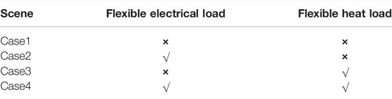
TABLE 1. Description of four scenarios.

Using MATLAB software to calculate the above four scenarios, in the improved multi-objective grey wolf algorithm, the total population is 100. The Pareto solution set convergence curves of the four scenarios are shown in Figure 3, and the optimization results are shown in Table 2.

FIGURE 3

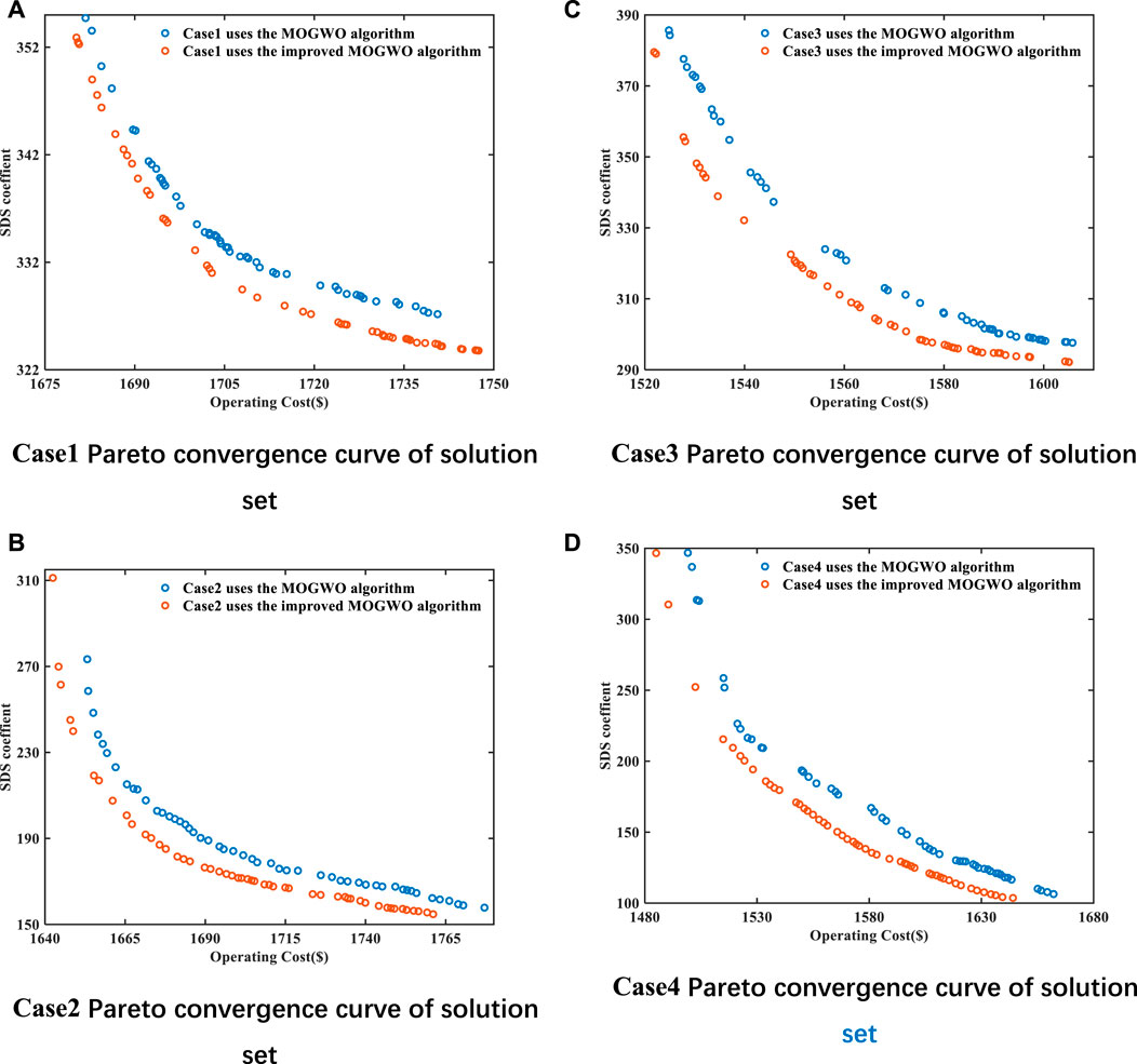
FIGURE 3. Convergence curves of Pareto solution sets in four scenarios. (A) Case1 Pareto convergence curve of solution set. (B) Case2 Pareto convergence curve of solution set. (C) Case3 Pareto convergence curve of solution set. (D) Case4 Pareto convergence curve of solution set.

TABLE 2

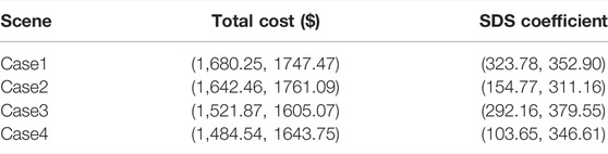
TABLE 2. Numerical range of optimization results of four scenarios.

It can be seen from the analysis in Figure 3 that the improved MOGWO has better convergence characteristics than the original MOGWO algorithm, and its search accuracy is also high. At the same time, due to the improvement of the update strategy of Pareto solution set, its diversity and distribution characteristics are better.

According to the analysis in Table 2, compared with traditional optimized operation (Case1), considering flexible electrical load and thermal load significantly improves the economy and stability of supply and demand of the system.

Considering the flexible electrical load (Case2), the total cost is only reduced by $37.79 compared to Case1, while the stability of supply and demand is improved by 52.20%. This is because the flexible electrical loads of Case2 can be time-shifted but not interrupted, and the time-shifted and interrupted electrical loads can improve the stability of supply and demand. However, the total load and energy supply form have not been greatly improved, so the cost cannot be effectively reduced. As for the curtailable electrical load, considering the user experience, the total amount of its participation in the demand response is small, and it can only slightly improve the system economy and the stability of supply and demand.

Considering the flexible heat load (Case3), the total cost is reduced by $158.38 compared to Case1, while the supply–demand stability factor is only increased by 9.77%. This is because the response of Case3’s flexible heat load heating mode turns electric heating to gas-heat central heating, which changes the energy supply form and reduces costs. For the curtailable electrical load, while adjusting the heat load curve to improving the stability of supply and demand, it avoids unnecessary waste of heat energy, thereby reducing costs. But similar to curtailable electrical loads, the effect is limited.

As for Case4, the advantages of Case2 and Case3 are taken into account because of both flexible electrical load and flexible thermal load, so that the economy and stability of supply and demand are optimal. The total cost was reduced by $195.71, and supply and demand stability improved by 67.99%.

7.2.1 Analysis of Electric Energy Operation Results

Select the scheme with the lowest total cost in Case1 ∼ Case4 and analyze the power operation results through comparison.

The power operation results of Case1 are shown in Figure 4A. During 1–6 and 23–24 electricity price valley/gas price peak period, electricity load is mainly borne by wind energy, large grid, and electric energy stored in EES. During the electricity price peak/gas price valley period from 7 to 12 and 19 to 22, the electricity load is mainly borne by gas turbines, wind energy, and large power grids, and electricity storage equipment releases electricity. During the electricity price average/gas price peak period from 13 to 18, the electricity load is mainly borne by gas turbines, wind energy, and large power grids, and the electricity storage equipment stores excess electricity. The output of the gas turbine decreases relative to the peak period of electricity price/valley gas price.

FIGURE 4

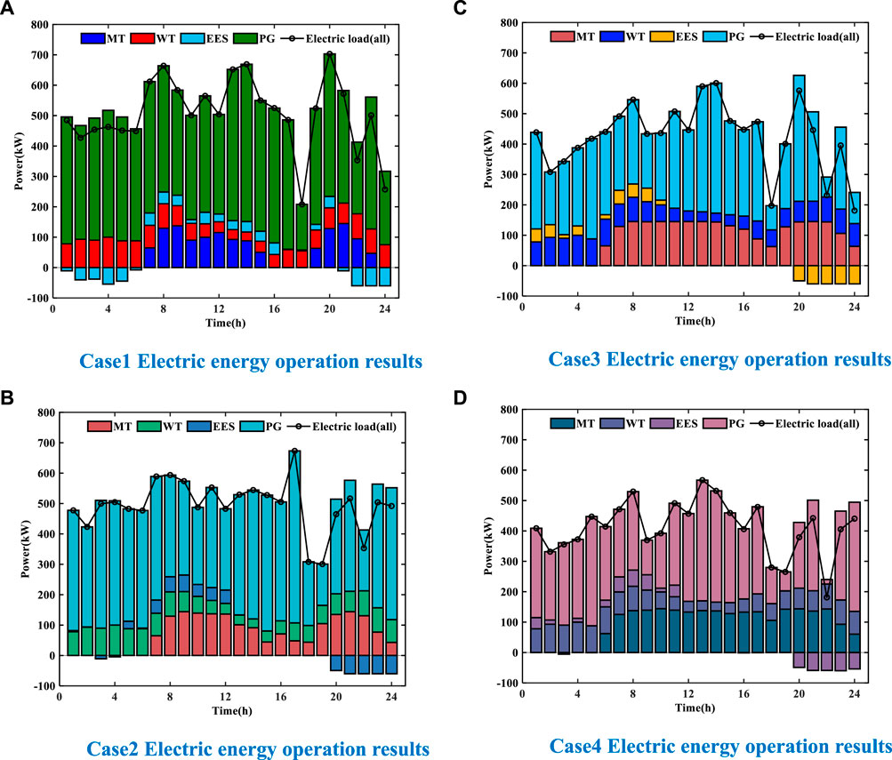
FIGURE 4. Case1–4 electric energy operation results. (A) Case1 electric energy operation results. (B) Case2 electric energy operation results. (C) Case3 electric energy operation results. (D) Case4 electric energy operation results.

The power operation results of Case2∼Case4 are shown in Figures 4B–D. Compared with Case1, in the periods 7–24, the electrical load borne by the gas turbine gradually increases, and the electrical load borne by the large power grid gradually decreases. During the periods 1–6, the stored electric energy of the power storage equipment decreased significantly, and during the periods 21–24, the released electric energy increased significantly.

7.2.2 Analysis of Thermal Energy Operation Results

Select the scheme with the smallest total cost in Case1∼Case4 and analyze the thermal energy operation results by comparison.

The power operation results of Case1 are shown in Figure 5A. During 1–6 and 23–24 electricity price valley/gas price peak period, the heat load is mainly borne by gas boilers and electric heating equipment. During the electricity price peak/gas price valley period from 7 to 12 and 19 to 22, the heat load is mainly borne by heat exchangers, gas boilers, and electric heating equipment. During the electricity price average/gas price peak period from 13 to 18, the heat load is mainly borne by heat exchangers, gas boilers, and electric heating equipment. Compared with the electricity price peak/gas price valley period, the output of the heat exchanger is reduced.

FIGURE 5

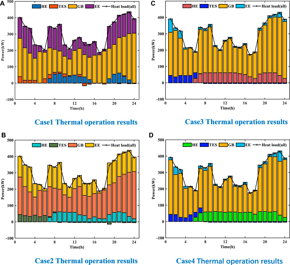
FIGURE 5. Case1–4 thermal operation results. (A) Case1 thermal operation results. (B) Case2 thermal operation results. (C) Case3 thermal operation results. (D) Case4 thermal operation results.

The thermal operation results of Case2∼Case4 are shown in Figures 5B–D. Compared with Case1, in the period of 7–24, the heat load borne by the heat exchanger gradually increases. During the whole period, the heat load borne by the gas boiler increased significantly.

7.2.3 Economic Analysis

In order to further analyze the influence of the improvement mentioned above on system economy, this paper conducts economic analysis by comparing Case1 to Case4.

The scheme with the lowest total cost from Case1 to Case4 was selected for economic analysis by comparison. The optimization results are shown in Table 3.

TABLE 3

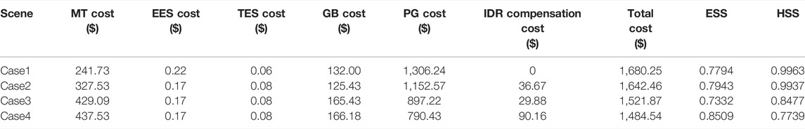
TABLE 3. Case1–4 economic-related indicators.

Combining Table 3 and Figure 6, the total cost of Case2 is reduced by $37.79 compared to that of Case1, of which the natural gas cost of the gas turbine is increased by $85.80 and that of the gas boiler is reduced by $6.57. The electricity purchase cost of the large grid decreased by $153.67; the aging costs of storage device were reduced by $0.03, which was negligible; an additional IDR compensation cost of $36.67 was incurred. This is because the load side of the Case2 system responds to demand by introducing flexible electrical loads to “cut peaks and fill valleys” for loads. It reduces the probability that the source-side gas turbine cannot supply energy in time due to factors such as ramp constraints, thereby increasing the natural gas cost of the gas turbine and indirectly reducing the power purchase cost of the large power grid.

FIGURE 6

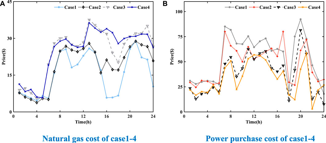
FIGURE 6. Natural gas cost and power purchase cost of Case1–4. (A) Natural gas cost of Case1–4. (B) Power purchase cost of Case1–4.

Compared with that of Case1, the total cost of Case3 decreased by 158.36 dollars, of which the natural gas cost of gas turbine and gas boiler increased by 187.36 dollars and 33.42 dollars, respectively, and the power purchase cost of large power grid decreased by 406.64 dollars. This is because the response of the load-side heating mode of the system makes some users change from electric heating to more economical gas-heat central heating. Therefore, the output proportion of gas-fired boiler and heat exchanger of natural gas equipment on the source side increases, which directly or indirectly increases the natural gas cost consumed by a gas turbine and gas-fired boiler and reduces the power purchase cost of large power networks.

Compared with Case1∼Case3, Case4 has the best economic indexes due to taking into account the above two advantages. The total cost decreased by $195.79. The cost of gas for the gas turbine and gas boiler increased by $195.71 and $34.18, respectively. The purchase of electricity by the large grid was reduced by $515.80. In addition, compared with Case1, Case4 increased the satisfaction of electricity consumption by 0.0715 and decreased the satisfaction degree of heat consumption by 0.2224. Among them, the improvement of power consumption satisfaction is because the load-side demand response makes users deviate from the power consumption time and the total amount but also improves the power generation adjustable rate. The reduction in heat satisfaction is smaller, similar to electricity satisfaction.

7.2.4 Analysis of Supply and Demand Stability

In order to further analyze the impact of the above improvements on the stability of supply and demand of the system, this paper conducts an analysis of the stability of supply and demand by comparing Case1∼Case4.

The scheme with the smallest supply and demand stability coefficient of Case1∼Case4 is selected, and the stability of supply and demand is analyzed by comparison. The optimization results are shown in Table 4.

TABLE 4

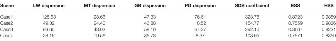
TABLE 4. Case1–4 indicators related to supply and demand stability.

As shown in Table 4, the overall supply and demand stability of Case2 is improved by 52.20% compared to that of Case1. The dispersion degree of LW, gas turbine, gas boiler, and large grid load curves decreased by 61.65%, 14.64%, 0.96%, and 75.51%, respectively. This is because the load side of the system reduces the dispersion degree of load curves of gas turbine, gas boiler, and large grid by introducing flexible electrical loads for demand response.

This is because the load side of the system performs demand response by introducing flexible electrical loads. While reducing the discrete degree of load curves of LW, gas boilers, and large power grids, more gas turbines are involved in power supply, which reduces the output stability of natural gas power generation equipment.

Compared with that of Case1, the overall supply and demand stability of Case3 is improved by 9.77%. The dispersion degree of LW and large grid load curves decreased by 22.53% and 10.90%, respectively, while the dispersion degree of gas turbine and gas boiler load curves increased by 50.13% and 22.94%, respectively. Obviously, the response of load side heating mode of the system not only reduces the dispersion of LW and large power grid load curve, but also makes natural gas heating equipment more involved in energy supply, thus improving the stability of its output.

Compared with that of Case1, the total stability of supply and demand of Case4 increased by 67.99%. The dispersion degree of LW, gas boilers, large power grids, and gas turbines decreases by 78.11%, 31.74%, 24.41%, and 88.92%, respectively. This is because the system load side avoids the adverse effects of Case1 and Case2 by introducing flexible electrical load and flexible thermal load to carry out demand response. Among them, the smoothness of LW curve was greatly improved, mainly reflected in the period from 7 to 24, as shown in Figure 7A. The smoothness of the gas turbine output curve has been greatly improved, mainly reflected in the periods 10–12, 15–19, and 1. The output curve is shown in Figure 7B. The smoothness of the output curve of the gas boiler has been improved to a certain extent as a whole, and its output curve is shown in Figure 7C. The smoothness of the output curve of the large power grid has been greatly improved as a whole, and the output curve is shown in Figure 7D.

FIGURE 7

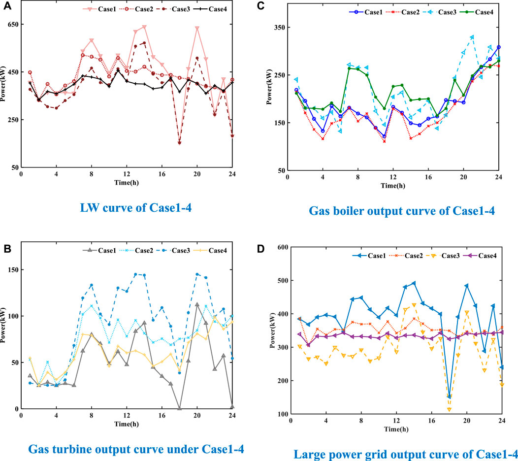
FIGURE 7. LW curve and output curve of large power grid, gas turbine, and gas boiler of Case1–4. (A) LW curve of Case1–4. (B) Gas turbine output curve of Case1–4. (C) Gas boiler output curve of Case1–4. (D) Large power grid output curve of Case1–4.

8 Conclusion

This paper proposes a multi-objective optimal source–load interaction scheduling of combined heat and power microgrid considering stable supply and demand. After comparing and analyzing the actual results, the conclusions are as follows:

1) The source side uses energy storage equipment to decouple the thermoelectric connection and introduces energy equipment to ensure the heating and power supply capacity of the system.

2) Flexible thermal and electrical loads are introduced on the load side for demand response, and an IDR compensation mechanism is established. It can effectively improve the economy of the system and the stability of supply and demand, in which the total cost is reduced by 11.65% and the stability of supply and demand is increased by 67.99%.

3) The comprehensive satisfaction evaluation system established by considering factors such as user energy deviation, IDR compensation price, supply-side heating, and power supply flexibility effectively guarantees the user’s comfort when participating in demand response.

4) The improved multi-objective grey wolf optimization algorithm adopted realizes the multi-objective optimal scheduling of the source–load interaction, promotes the benign interaction between the system source and the load, and ensures the supply and demand stability and economy of the CHP-MG operation.

This paper discusses the benign interaction between the source and the load of microgrid system, which is suitable for the cooperative planning of energy equipment in the system. However, for other large-scale industrial systems, the fault diagnosis and monitoring of internal equipment (Rui et al., 2020b; Hu et al., 2021) has not been taken into consideration, and further research is needed in the future.

Data Availability Statement

The original contributions presented in the study are included in the article/Supplementary Material, further inquiries can be directed to the corresponding author.

Author Contributions

JC and XY conceived and designed the study. JC constructed and solved the model and wrote the first draft of the manuscript. ZZ and SZ translated the article and drew the tables. BC drew the schematic diagrams. All authors contributed to revision of the manuscript and read and approved the submitted version.

Conflict of Interest

The authors declare that the research was conducted in the absence of any commercial or financial relationships that could be construed as a potential conflict of interest.

Publisher’s Note

All claims expressed in this article are solely those of the authors and do not necessarily represent those of their affiliated organizations, or those of the publisher, the editors, and the reviewers. Any product that may be evaluated in this article, or claim that may be made by its manufacturer, is not guaranteed or endorsed by the publisher.

Supplementary Material

The Supplementary Material for this article can be found online at: https://www.frontiersin.org/articles/10.3389/fenrg.2022.901529/full#supplementary-material

References

Aghamohammadloo, H., Talaeizadeh, V., Shahanaghi, K., Aghaei, J., Shayanfar, H., Shafie-khah, M., et al. (2021). Integrated Demand Response Programs and Energy Hubs Retail Energy Market Modelling. J. Energy, 234. doi:10.1016/j.energy.2021.121239

CrossRef Full Text | Google Scholar

Alomoush, M. I. (2019). Microgrid Combined Power-Heat Economic-Emission Dispatch Considering Stochastic Renewable Energy Resources, Power Purchase and Emission Tax. Energy Convers. Manag. 200, 112090. doi:10.1016/j.enconman.2019.112090

CrossRef Full Text | Google Scholar

Amir, V., Jadid, S., and Ehsan, M. (2019). Operation of Networked Multi-Carrier Microgrid Considering Demand response[J]. England: Compel Int J for Computation & Maths in Electrical & Electronic Eng.

Google Scholar

Anh, H., and Cao, V. K. (2020). Optimal Energy Management of Microgrid Using Advanced Multi-Objective Particle Swarm optimization[J]. Wales: Engineering Computations.

Google Scholar

Blair, M. J., and Mabee, W. E. (2020). Evaluation of Technology, Economics and Emissions Impacts of Community-Scale Bioenergy Systems for a Forest-Based Community in Ontario. Renew. Energy 151, 715–730. doi:10.1016/j.renene.2019.11.073

CrossRef Full Text | Google Scholar

Dranka, G. G., Ferreira, P., and Vaz, A. (2021). Integrating Supply and Demand-Side Management in Renewable-Based Energy systems[J]. England: Energy, 120978.

CrossRef Full Text | Google Scholar

Freeman, J., Hellgardt, K., and Markides, C. N. (2017). Working Fluid Selection and Electrical Performance Optimisation of a Domestic Solar-ORC Combined Heat and Power System for Year-Round Operation in the UK. Appl. Energy 186 (3), 291–303. doi:10.1016/j.apenergy.2016.04.041

CrossRef Full Text | Google Scholar

Hca, B., Lin, G., and Zhong, Z. C. (2021). Multi-objective Optimal Scheduling of a Microgrid with Uncertainties of Renewable Power Generation Considering User Satisfaction[J]. Int. J. Electr. Power & Energy Syst. 131.

Google Scholar

Hemmati, M., Mirzaei, M. A., Abapour, M., Zare, K., Mohammadi-ivatloo, B., Mehrjerdi, H., et al. (2021). Economic-environmental Analysis of Combined Heat and Power-Based Reconfigurable Microgrid Integrated with Multiple Energy Storage and Demand Response Program. Sustain. Cities Soc. 69, 102790. doi:10.1016/j.scs.2021.102790

CrossRef Full Text | Google Scholar

Hemmati, R., Mehrjerdi, H., and Nosratabadi, S. M. (2021). Resilience-oriented Adaptable Microgrid Formation in Integrated Electricity-Gas System with Deployment of Multiple Energy Hubs. Sustain. Cities Soc. 71 (3), 102946. doi:10.1016/j.scs.2021.102946

CrossRef Full Text | Google Scholar

Hu, X., Zhang, H., Ma, D., and Wang, R. (2021). Hierarchical Pressure Data Recovery for Pipeline Network via Generative Adversarial Networks. IEEE Trans. Autom. Sci. Eng. (99), 1–11. doi:10.1109/tase.2021.3069003

CrossRef Full Text | Google Scholar

Ippolito, F., and Venturini, M. (2018). Development of a Simulation Model of Transient Operation of Micro-combined Heat and Power Systems in a Microgrid[J]. J. Eng. Gas Turbines Power 140 (3), 032001.1–032001.15. doi:10.1115/1.4037962

CrossRef Full Text | Google Scholar

Jiang, Y., Mei, F., Lu, J., and Lu, J. (2021). Two-Stage Joint Optimal Scheduling of a Distribution Network with Integrated Energy Systems. IEEE Access 9, 12555–12566. doi:10.1109/access.2021.3051351

CrossRef Full Text | Google Scholar

Jordehi, A. R . (2021). Information Gap Decision Theory for Operation of Combined Cooling, Heat and Power Microgrids with Battery Charging stations[J]. Netherlands: Sustainable Cities and Society.

Google Scholar

Kennedy, J., and Eberhart, R. (1995). Particle Swarm Optimization[C]//Icnn95-International Conference on Neural Networks. IEEE.

Google Scholar

Li, P., Wang, Z., Wang, J., Yang, W., Guo, T., and Yin, Y. (2021). Two-stage Optimal Operation of Integrated Energy System Considering Multiple Uncertainties and Integrated Demand Response. Energy 225 (4), 120256. doi:10.1016/j.energy.2021.120256

CrossRef Full Text | Google Scholar

Li, Y., Han, M., and Yang, Z. (2021). Coordinating Flexible Demand Response and Renewable Uncertainties for Scheduling of Community Integrated Energy Systems with an Electric Vehicle Charging Station: A Bi-level Approach[J].

Google Scholar

Li, Y., Wang, B., and Yang, Z. (2021). Optimal Scheduling of Integrated Demand Response-Enabled Community Integrated Energy Systems in Uncertain Environments[J].

Google Scholar

Li, Y., Zhang, J., Ma, Z., Peng, Y., and Zhao, S. (2021). An Energy Management Optimization Method for Community Integrated Energy System Based on User Dominated Demand Side Response[J]. Energies, 14.

Google Scholar

Li, Y., Zhang, H., Liang, X., and Huang, B. (2019). Event-Triggered-Based Distributed Cooperative Energy Management for Multienergy Systems. IEEE Trans. Ind. Inf. 15 (4), 2008–2022. doi:10.1109/TII.2018.2862436

CrossRef Full Text | Google Scholar

Liu, L., and Yang, G.-H. (2022). Distributed Optimal Energy Management for Integrated Energy Systems. IEEE Trans. Ind. Inf., 1. doi:10.1109/TII.2022.3146165

CrossRef Full Text | Google Scholar

Liu, N., Wang, J., and Wang, L. (2018). Hybrid Energy Sharing for Multiple Microgrids in an Integrated Heat-Electricity Energy System[J]. IEEE Trans. Sustain. Energy 10 (3), 1139–1151.

Google Scholar

Lu, J., Liu, T., and He, C.. Robust Day-Ahead Coordinated Scheduling of Multi-Energy Systems with Integrated Heat-Electricity Demand Response and High Penetration of Renewable Energy[J]. Renew. Energy 2021 (1).

Google Scholar

Lv, H., Wang, Y., and Dong, X. (2021). Optimization Scheduling of Integrated Energy System Considering Demand Response and Coupling Degree[C]//2021 IEEE/IAS 57th Industrial and Commercial Power Systems Technical Conference (I&CPS). IEEE.

Google Scholar

Mirjalili, S., Saremi, S., Mirjalili, S. M., and Coelho, L. S. (2016). Multi-Objective Grey Wolf Optimizer: A Novel Algorithm for Multi-Criterion Optimization[J]. Expert Syst. Appl. 47, 106–119.

CrossRef Full Text | Google Scholar

Mirjalili, S., Mirjalili, S. M., and Lewis, A. (2014). Grey Wolf Optimizer[J]. Adv. Eng. Softw., 46–61.

CrossRef Full Text | Google Scholar

Mohseni, S., Brent, A. C., and Kelly, S. (2021). Strategic Design Optimisation of Multi-Energy-Storage-Technology Micro-grids Considering a Two-Stage Game-Theoretic Market for Demand Response aggregation[J]. England: Applied Energy, 287.

Google Scholar

Munoz-Delgado, G., Contreras, J., and Arroyo, J. M. (2016). Multistage Generation and Network Expansion Planning in Distribution Systems Considering Uncertainty and Reliability. IEEE Trans. Power Syst. 31 (5), 3715–3728. doi:10.1109/tpwrs.2015.2503604

CrossRef Full Text | Google Scholar

Naderipour, A., Abdul-Malek, Z., and Nowdeh, S. A. (2020). Optimal Allocation for Combined Heat and Power System with Respect to Maximum Allowable Capacity for Reduced Losses and Improved Voltage Profile and Reliability of Microgrids Considering Loading Condition[J]. Energy 196 (Apr.1), 117124.1–117124.13. doi:10.1016/j.energy.2020.117124

CrossRef Full Text | Google Scholar

Nojavan, S., Akbari-Dibavar, A., Farahmand-Zahed, A., and Zare, K. (2020). Risk-constrained Scheduling of a CHP-Based Microgrid Including Hydrogen Energy Storage Using Robust Optimization Approach. Int. J. Hydrogen Energy 45 (56), 32269–32284. doi:10.1016/j.ijhydene.2020.08.227

CrossRef Full Text | Google Scholar

Pashaei-Didani, H., Nojavan, S., Nourollahi, R., and Zare, K. (2019). Optimal Economic-Emission Performance of Fuel cell/CHP/storage Based Microgrid. Int. J. hydrogen energy 44 (13), 6896–6908. doi:10.1016/j.ijhydene.2019.01.201

CrossRef Full Text | Google Scholar

Ronaszegi, K., Fraga, E. S., Darr, J., Shearing, P. R., and Brett, D. J. L. (2020). Application of Photo-Electrochemically Generated Hydrogen with Fuel Cell Based Micro-combined Heat and Power: A Dynamic System Modelling Study. Molecules 25 (1). doi:10.3390/molecules25010123

PubMed Abstract | CrossRef Full Text | Google Scholar

Rui, W., Qiuye, S., Pinjia, Z., Yonghao, G., Dehao, Q., and Peng, W. (2020). Reduced-Order Transfer Function Model of the Droop-Controlled Inverter via Jordan Continued-Fraction Expansion. IEEE Trans. Energy Convers. 35 (3), 1585–1595. doi:10.1109/TEC.2020.2980033

CrossRef Full Text | Google Scholar

Rui, W., Qiuye, S., Pinjia, Z., Yonghao, G., Dehao, Q., and Peng, W. (2020). Reduced-Order Transfer Function Model of the Droop-Controlled Inverter via Jordan Continued-Fraction Expansion. IEEE Trans. Energy Convers. 35 (3), 1585–1595. doi:10.1109/TEC.2020.2980033

CrossRef Full Text | Google Scholar

Salama, H. S., Said, S. M., and Aly, M. (2021). Studying Impacts of Electric Vehicle Functionalities in Wind Energy-Powered Utility Grids with Energy Storage Device[J]. IEEE Access (99), 1.

Google Scholar

Salehimaleh, M., Akbarimajd, A., and Dejamkhooy, A. (2022). A Shrinking-Horizon Optimization Framework for Energy Hub Scheduling in the Presence of Wind Turbine and Integrated Demand Response Program.

Google Scholar

Shao, C., Ding, Y., and Siano, P. (2020). Optimal Scheduling of the Integrated Electricity and Natural Gas Systems Considering the Integrated Demand Response of Energy Hubs[J]. IEEE Syst. J. (99), 1–9.

Google Scholar

Singh, S., and Kumar, A. (2020). Economic Dispatch for Multi Heat-Electric Energy Source Based microgrid[C]//2020 IEEE 9th Power India International Conference (PIICON). IEEE.

Google Scholar

Taha, I., and Elattar, E. E. (2018). “Optimal Reactive Power Resources Sizing for Power System Operations Enhancement Based on Improved Grey Wolf Optimiser[J],” in IET Generation (England: Transmission & Distribution). doi:10.1049/iet-gtd.2018.0053

CrossRef Full Text | Google Scholar

Wang, J., Liu, J., Li, C., Zhou, Y., and Wu, J. (2020). Optimal Scheduling of Gas and Electricity Consumption in a Smart Home with a Hybrid Gas Boiler and Electric Heating System. Energy 204, 117951. doi:10.1016/j.energy.2020.117951

CrossRef Full Text | Google Scholar

Wang, R., Sun, Q., Hu, W., Li, Y., Ma, D., and Wang, P. (2021). SoC-Based Droop Coefficients Stability Region Analysis of the Battery for Stand-Alone Supply Systems with Constant Power Loads. IEEE Trans. Power Electron. 36 (7), 7866–7879. doi:10.1109/TPEL.2021.3049241

CrossRef Full Text | Google Scholar

Wang, R., Sun, Q., Tu, P., Xiao, J., Gui, Y., and Wang, P. (2021). Reduced-Order Aggregate Model for Large-Scale Converters with Inhomogeneous Initial Conditions in DC Microgrids. IEEE Trans. Energy Convers. 36 (3), 2473–2484. doi:10.1109/TEC.2021.3050434

CrossRef Full Text | Google Scholar

Wc, A., Xiao, P. B., and Bs, C. (2021). Integrated Demand Response Based on Household and Photovoltaic Load and Oscillations Effects.

Google Scholar

Yang, B., Yu, T., Shu, H., Dong, J., and Jiang, L. (2018). Robust Sliding-Mode Control of Wind Energy Conversion Systems for Optimal Power Extraction via Nonlinear Perturbation Observers[J]. Appl. Energy 210, 711–723.

CrossRef Full Text | Google Scholar

Yang, J., Huang, G., and Wei, C. (2016). Privacy-aware Electricity Scheduling for Home Energy Management System[J]. Peer-to-Peer Netw. Appl..

Google Scholar

Yang, L., Yang, Z., and Li, G. (2019). Optimal Scheduling of an Isolated Microgrid with Battery Storage Considering Load and Renewable Generation Uncertainties[J]. IEEE Trans. Industrial Electron. 66, 1565–1575.

CrossRef Full Text | Google Scholar

Yi, Z., Xu, Y., Hu, J., Chow, M.-Y., and Sun, H. (2020). Distributed, Neurodynamic-Based Approach for Economic Dispatch in an Integrated Energy System. IEEE Trans. Ind. Inf. 16 (4), 2245–2257. doi:10.1109/TII.2019.2905156

CrossRef Full Text | Google Scholar

Zhang, S., Rong, J., and Wang, B. (2021). An Optimal Scheduling Scheme for Smart Home Electricity Considering Demand Response and Privacy Protection. Int. J. Electr. Power & Energy Syst. 132 (4), 107159. doi:10.1016/j.ijepes.2021.107159

CrossRef Full Text | Google Scholar

Zhang, X., Shahidehpour, M., and Alabdulwahab, A. (2015). Hourly Electricity Demand Response in the Stochastic Day-Ahead Scheduling of Coordinated Electricity and Natural Gas Networks[J]. IEEE Trans. Power Syst. 31 (1), 592–601.

Google Scholar

Zhang, Y., Shen, H., and Wen, J. (2019). Storage Control of Integrated Energy System for Integrated Demand Response[J]. Beijing, China: Electric Power Construction.

Google Scholar

Zhao, D., Xia, X., and Tao, R. (2019). Optimal Configuration of Electric/Thermal Integrated Energy Storage for Combined Heat and Power Microgrid with Power to Gas[J]. Nanjing, China: Automation of Electric Power Systems.

Google Scholar

Zhou, C. (2019). Operation Optimization of Multi-District Integrated Energy System Considering Flexible Demand Response of Electric and Thermal Loads. Energies 12. doi:10.3390/en12203831

CrossRef Full Text | Google Scholar

Nomenclature

CHP-MG Combined heat and power microgrid

SDS Supply and demand stability

ESS Power supply satisfaction

HSS Heat supply satisfaction

IDR Integrated demand response

LW Electrical load–wind energy

WT Wind turbine

MT Micro-turbine

GB Gas boiler

EES Electrical energy storage

TES Thermal energy storage

HE Heat exchanger

EE Electrothermal equipment

PG Power grid

$P_{WT}^t$ Generated power of wind turbine in time period t

$P_{MT}^t$ Electric generation power of micro-turbine in period t

$Q_{HE}^t$ Heat production power of heat exchanger in period t

$Q_{GB}^t$ Heat production power of gas boiler in period t

$Q_{EE}^t$ Heat production power of electrothermal equipment in period t

$E_{EES}^t$ Storage capacity of electrical energy storage in period t

$E_{TES}^t$ Storage capacity of thermal energy storage in period t