Evaluating the significance of samples in deep learning-based transient stability assessment

1 Introduction

Transient stability assessment (TSA) has always been an active research topic since transient instability is one of the major threats to a power system. Prior research on TSA can be roughly categorized into two aspects, i.e. the time-domain simulation and the direct method (Kundur, 1994). Time-domain simulation computes the state trajectories through numerical integration. With the increasing penetration of the converter-interfaced generation (CIG), it has become infeasible and time consuming to carry out scalable electro-magnetic transient simulations. The direct methods for TSA utilize the Lyapunov theory to analyze the geometric properties and determine the region of attraction of the power system. The core task of the direct methods is to find the Lyapunov function, which is only known for a limited class of power system models and has no general methods to construct.

During the past decade, inspired by the tremendous success in computer vision and the natural language-processing field, researchers started to apply the deep learning techniques in power system TSA. Various network structures and algorithms have been applied in the TSA analysis, including the deep belief network (DBN) (Zheng et al., 2018; Wu et al., 2020), the convolutional neural network (CNN) (Azman et al., 2020; Shi et al., 2020; Zhu et al., 2020), the long short-term memory (LSTM) network (Azman et al., 2020; Sun et al., 2020; Hagmar et al., 2021), the generative adversarial network (GAN) (Yang et al., 2021), the feature-separated neural network (Zhou et al., 2021), etc. In all these research studies, the first step is to create a dataset by time-domain simulations considering various operating conditions and transient faults. The deep learning model has multiple layers and is often over-parameterized, so it is preferred to train the models on ever larger datasets to avoid over-fitting. Since time-domain simulations are very time-consuming for large power systems, this trend poses much larger computational burden and hardware resource requirement. Days and even months are needed to prepare the dataset for training TSA models. It is of theoretical and practical interest to understand how an individual sample influences the learning process, so as to prune less important training data and shrink the dataset.

The artificial intelligence (AI) community has made some interesting attempts in this direction (Campbell and Broderick, 2018; Toneva et al., 2019; Hwang et al., 2020; Paul et al., 2021). The basic idea is to identify certain subsets that allows training and maintaining almost the same accuracy with the original full dataset (Campbell and Broderick, 2018; Hwang et al., 2020). However, due to the non-convex nature of machine learning algorithms and a huge number of samples, random search is less effective in practice and lacks theoretical guarantees. Toneva et al. (2019) propose a very different approach. They track the number of flippings that a sample is classified from one label to the other or vice versa through the training process. It is observed that the samples that rarely flip have little impact on the test accuracy after removing. On the contrary, the samples flipping many times are important to the test. Therefore, the number of flippings is taken as the significance criteria for the samples. The idea is very intuitive, indicating that the contribution of a sample to the decrease of loss is highly related to the significance of the sample. Considering that deep learning models are usually trained with the stochastic gradient decent (SGD) algorithm, Paul et al. (2021) prove that the expected change in loss of any individual sample is bounded by the expected loss gradient norm, which can be approximated by the norm of the error vector.

Following the technique proposed by Paul et al., 2021, an empirical study of the sample significance index in TSA is proposed. To the best of our knowledge, this article is the first to study the significance of samples in the deep learning-based TSA analysis, which will lead to new methodologies that could dramatically reduce dataset generation time and training efforts. In addition, it offers important insights into the training dynamics of deep neural networks and potential interpretable capability for the deep learning-based TSA. The rest of the article is organized as follows. Firstly, the article describes the preliminaries on the expected loss gradient norm and how to compute the Sample Significance Index (SSI) and the stability score. An illustrative example using the single-machine infinite-bus (SMIB) system will be presented in the next section. The case study gives more results on the effect of dataset pruning with various deep learning models, subset sizes, SSI thresholds, and noisy levels. The last section concludes the article and points out future directions.

2 The sample significance index and the stability score

2.1 Dataset generation in TSA

In the machine learning-based TSA analysis, it is often formulated as a supervised classification problem. The first step is to generate the dataset used for training and testing, denoted by $S={\left\{(x_i,y_i)\right\}}_{i=1}^N$, with the input features $x\in {ℝ}^d$ and the one-hot encoded labels $y\in {\left\{\mathrm{0,1}\right\}}^K$. Given a specific system, a multitude of operating conditions and transient faults are pre-defined. Then, thorough time-domain simulations are carried to generate the samples. The most frequently used label y is the stability status after the transient faults, and K = 2 since the system will be either stable or unstable. The input features x are various in different studies, including the angle and magnitude of the bus voltage, the active and reactive power in the transmission line, the power angle and rotor speed of the generator, etc.

To reliably determine the stability status, the simulation duration is often set to 10 s or more. And the input feature is also high- dimensional. Therefore, the dataset generation stage is the most time- and computational resource-consuming step if the dataset size is large. It is necessary to seek the answer to the question of what is the nature of samples that can be removed from the training dataset without hurting the accuracy.

2.2 The expected gradient norm score

The following definition and derivation are mainly taken from (Paul et al., 2021). For fixed neural network architecture, let $p(\text{w},x)\in {ℝ}^2$ be the outputs of the neural network in the form of a probability vector and $\text{w}$ represents the weights of the network. Suppose the loss function is the cross-entropy loss:

$\ell \left(p,y\right)={\displaystyle {\sum }_{k=1}^2{y}^{\left(k\right)}\log p^{\left(k\right)}}(1)$

Let ${\mathbf{w}}_0,{\mathbf{w}}_1,{\mathbf{w}}_2,\cdots ,{\mathbf{w}}_T$ be the iterates of weights through the SGD, and by definition we have:

$\begin{array}{c}{\mathbf{w}}_t={\mathbf{w}}_{t-1}-\mathit{\eta }{\displaystyle {\sum }_{(x,y)\in S}{g}_{t-1}\left(x,y\right)}\\ ={\mathbf{w}}_{t-1}-\mathit{\eta }{\displaystyle {\sum }_{(x,y)\in S}{\nabla }_{{\text{w}}_{t-1}}\ell \left(p\left({\mathbf{w}}_{t-1},x\right),y\right)}\end{array}(2)$

where $t=\mathrm{1,2},\cdots ,T$ denotes the index of the training iteration, $\mathit{\eta }$ is the learning rate, and $g_{t-1}(x,y)$ is the gradient of the loss function to the weights:

$g_{t-1}\left(x,y\right)={\nabla }_{{\text{w}}_{t-1}}\ell \left(p\left({\mathbf{w}}_{t-1},x\right),y\right)(3)$

In order to simplify the analysis, the discrete training iterations are approximated as continuous training dynamics. The loss change along the training iterations can then be represented as the time derivative of the loss function:

${\mathrm{\Delta }}_t\left(\left(x,y\right),S\right)=-\frac{d}{dt}\ell \left(p\left({\mathbf{w}}_t,x\right),y\right)(4)$

Following the chain rule, we can get

$\begin{array}{c}{\mathrm{\Delta }}_t((x,y),S)=-\frac{d\ell \left(p\left({\mathbf{w}}_t,x\right),y\right)}{d{\mathbf{w}}_t}\cdot \frac{d{\mathbf{w}}_t}{dt}\\ \approx -\frac{d\ell \left(p\left({\mathbf{w}}_t,x\right),y\right)}{d{\mathbf{w}}_t}\cdot \left({\mathbf{w}}_{t+1}-{\mathbf{w}}_t\right)\\ =\frac{d\ell \left(p\left({\mathbf{w}}_t,x\right),y\right)}{d{\mathbf{w}}_t}\cdot \mathit{\eta }{\displaystyle {\sum }_{(x,y)\in S}{g}_t\left(x,y\right)}\end{array}(5)$

Then, if we remove any sample $(x_j,y_j)$ from the training set S at iteration step t, the contribution of the training sample to the loss change can be derived as:

$\begin{array}{l}\Vert {\mathrm{\Delta }}_t\left(\left(x,y\right),S\right)-{\mathrm{\Delta }}_t\left(\left(x,y\right),S_{-j}\right)\Vert \\ =\Vert \mathit{\eta }\frac{d\ell }{d{\mathbf{w}}_t}{\displaystyle {\sum }_{\left(x,y\right)\in S}{g}_t\left(x,y\right)}-\mathit{\eta }\frac{d{\ell }^{\prime }}{d{\mathbf{w}}_t}{\displaystyle {\sum }_{\left(x,y\right)\in S_{-j}}{g}_t\left(x,y\right)}\Vert \\ \le \mathit{\eta }\Vert \frac{d\ell }{d{\mathbf{w}}_t}\Vert \cdot \Vert g_t\left(x_j,y_j\right)\Vert =c\Vert g_t\left(x_j,y_j\right)\Vert \end{array}(6)$

Therefore, the contribution of a training sample to the loss change is bounded by Eq. 6. Since the constant c does not depend on $\left(x_j,y_j\right)$, the gradient norm term $\Vert g_t\left(x_j,y_j\right)\Vert$ is of more interest. Since the weights are initialized with random variables, we define the expected value of the gradient norm, which is called the GraNd score in Paul et al., 2021.

${\mathit{\chi }}_{\mathit{t}}\left(\mathit{x,y}\right)\mathrm{=}{\mathbb{E}}_{{\mathbf{w}}_{\mathit{t}}}{\Vert g_{\mathbf{t}}\left(\mathrm{x,y}\right)\Vert }_{\mathrm{2}}(7)$

The GraNd score describes the contribution of a sample to the change in the training loss. Specifically, samples with a small GraNd score in expectation have a limited influence on the training process. Note that the opposite is not necessarily true since Eq. 6 only gives an upper bound. We will see some examples in the case study section.

2.3 The norm of the error vector score

Let $f(\text{w},x)\in {ℝ}^2$ be the neuron outputs of the second-last layer of the neural network, and the last layer is a Softmax layer, then the relation between f and p is

$p^{\left(k\right)}\left(\mathbf{w},x\right)=\exp \left(f^{\left(k\right)}\left(\mathbf{w},x\right)\right)/{\displaystyle {\sum }_{i=1}^2\exp \left(f^{\left(i\right)}\left(\mathbf{w},x\right)\right)}(8)$

Taking Eq. 3 and the chain rule, g_t is converted to:

$g_t\left(x,y\right)={\nabla }_f\ell {\left(f\left({\mathbf{w}}_t,x\right),y\right)}^T\cdot {\nabla }_{{\text{w}}_t}f\left({\mathbf{w}}_t,x\right)(9)$

Substitute Eq. 8 into Eq. 1, it is easy to get:

${\nabla }_f\ell {\left(f\left({\mathbf{w}}_t,x\right),y\right)}^T=p\left({\mathbf{w}}_t,x\right)-y(10)$

Therefore, the GraNd score is:

${\mathit{\chi }}_{\mathit{t}}\left(\mathit{x,y}\right)\mathrm{=}\mathbb{E}{\Vert \mathit{p}\left({\mathbf{w}}_{\mathrm{t}},x\right)\mathrm{-}y\Vert }_{\mathrm{2}}\mathrm{\cdot }\mathbb{E}{\Vert {\mathrm{\nabla }}_{{\mathbf{w}}_{\mathit{t}}}\mathit{f}\left({\mathbf{w}}_{\mathrm{t}}\mathrm{,}\mathrm{x}\right)\Vert }_{\mathrm{2}}(11)$

The right part of Eq. 11 is of a similar size across the logits and samples (Paul et al., 2021), so the GraNd score can be approximated by the norm of the error vector, which is called the Sample Significance Index (SSI) in this article Eq. 12.

$\mathit{SSI=}\mathbb{E}{\Vert \mathit{p}\left({\mathbf{w}}_{\mathit{t}}\mathit{,x}\right)\mathit{-y}\Vert }_{\mathrm{2}}(12)$

Therefore, an easy-to-compute criteria SSI is proposed to evaluate the upper bound of the contribution of any sample to the loss change of the neural network during the training process.

2.4 The stability score

The stability degree of a given sample is usually measured by the difference between the fault-clearing time (CT) and critical-clearing time (CCT). However, there are some difficulties to get the CCT of complex systems, such as the accuracy and fast computation speed (Sulistiawati et al., 2016). In the experiment of a single-machine infinite system, we find that the high Sample Significance Index samples are concentrated on the stable boundary, while the low index samples are far away from it, which is tenable for complex systems as the follow-up experiment shows. According to the SSI definition, the SSI of the samples that is easy to distinguish is significantly lower than those prone to misjudgment and far from the stability boundary in the sample space. So, in the training process, combining the distribution of SSI, we propose the stability score which could be used to evaluate the degree of sample stability as a secondary criterion for assessment.

We standardize the index at first as:

$\mathit{SSI}\_\mathit{norm}\mathrm{=}\frac{\mathit{SSI}\mathrm{-min}\left(\mathit{SSI}\right)}{\max \left(\mathit{SSI}\right)\mathrm{-min}\left(\mathit{SSI}\right)}(13)$

And we get the stability score:

$StabilityScore=\{\begin{array}{cc}{\left(-1\right)}^{a_{stable}}\lg \left(SSI\_norm\right)& \left(0<SSI\_norm\le 1\right)\\ {\left(-1\right)}^{a_{stable}}\left(m_{score}-1\right)& \left(SSI\_norm=0\right)\end{array}(14)$

In Eq. 14, $a_{stable}$ represents the model judgment result. If the model judges the sample to be stable, the value of $a_{stable}$ is 1. Otherwise, it is 0. And, $m_{score}$ is calculated by $m_{score}=\min \left(\lg (SSI\_norm)\right)$ in which $0<SSI\_norm\le 1$.

2.5 The procedure to evaluate the SSI and stability score

The SSI and stability score could be calculated by the following three steps, as Figure 1 shows:

FIGURE 1

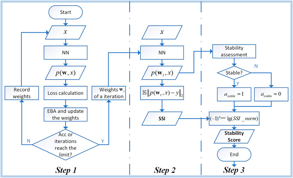
FIGURE 1. The procedure to evaluate the significance and stability.

Step 1: Input the training dataset into a neural network of which the parameters of each epoch are recorded during the training. Then, calculate the output error which is propagated back and adjust the weights of the neuron. And the end of the training is marked by the accuracy rate or the number of iterations reaching the set standard.

Step 2: The neural network parameters of an iteration to calculate SSI are imported to the network again and input the samples to the neural network. The output and the labels of the training sample are calculated by Eq. 12. And here we get the Significance Index.

Step 3: The output of step 2’s neural network is used as the input of the stability assessment of the sample. And parameter $a_{stable}$ is defined according to the stability of the sample. Finally the stability score of the sample is calculated by using Eq. 14 together with SSI.

3 An illustrative example

In the power system TSA tasks, the knowledge learned from machine learning algorithms is usually interpreted as the stability boundary (Zheng et al., 2018). In this section, we will evaluate the SSI generated from a SMIB system, and the parameters are given in Supplementary Table S1. Since the real stability boundary can be easily computed in a 2D plane, we can evaluate the links between the SSI and the distance to the stability boundary of an individual sample from the training dataset in an intuitive way.

The input feature includes the power angle and the rotor speed of the generator. 4,000 samples are randomly generated from the state space. A 4-layer multiple layer perceptron (MLP) is trained 200 epochs and the SSI are computed at each training epoch. The results are shown in Figure 2A. The dashed red line denotes the theoretical stability boundary of the SMIB system whereas the Sample Significance Indexes from the epoch 90 are marked by colors. It is easy to see the trend where the samples away from the boundary have relatively low SSI, meaning that those samples are less important to the training process. Then, we sort the samples by SSI and eliminate 50% of the low-index samples which are far from the stable boundary as shown in Figure 2B. The remaining samples are distributed around the stable boundary. The SSI change little from before, however, the SSI of the samples closed to boundary increase, that is, they are more prone to be misclassified. The slight change is also reflected in the decrease of test accuracy.

FIGURE 2

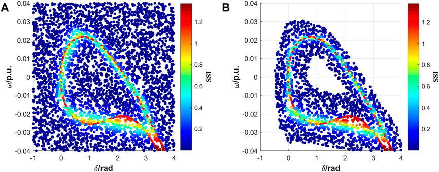
FIGURE 2. SSI at epoch 90 of the SMIB system. (A) shows the SSI of the full dataset and (B) shows the SSI of the subset after pruning.

Figure 3 shows the index distribution of different training epochs. We observe that the SSI distribution becomes long-tailed quickly during the training stage (Figures 3A–C). Then, we categorize the samples into two groups. The low-index group contains samples with SSI smaller than the 90% quantile of all SSI at epoch 90, while the high-index group contains all the other samples. From Figure 3D, it can be seen that the low-index group becomes stable quickly after a few epochs and the index variation is small. However, the SSI of the high-index group has a relatively large vibration until around epoch 90. This indicates that the sample significance can be determined during the training stage, instead of at the end of training as in Toneva et al., 2019. Considering that the training process often has hundreds even thousands of iterations, it is possible to prune the dataset very early, thus saving computational effort and time.

FIGURE 3

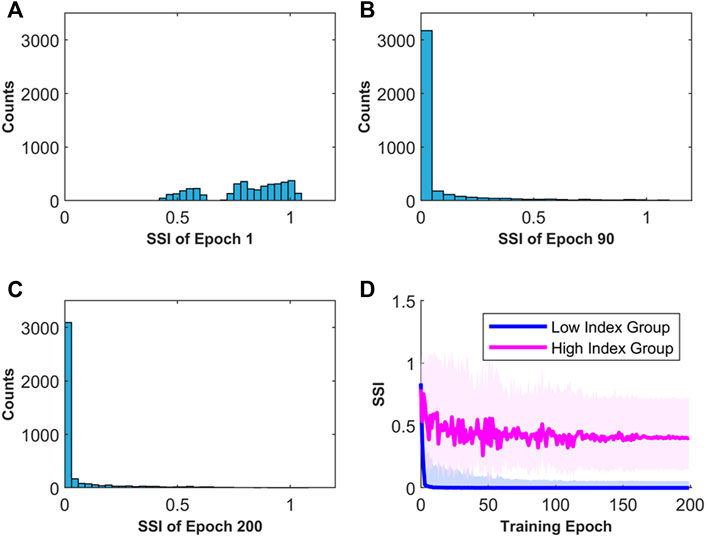
FIGURE 3. Sample Significance Index distribution along the training epochs. (A) SSI distribution at epoch 1. (B) SSI distribution at epoch 90. (C) SSI distribution at epoch 200. (D) Median SSI curve for the low- and high-index groups. The light-colored area shows the 10–90% quantiles of the indexes.

The stability scores are calculated according to Eqs 12, 13. In order to facilitate the study, scores of stable samples and unstable samples are mapped to $[-\mathrm{1,0})$ and $\left[\mathrm{0,1}\right]$, respectively, as shown in Figure 4. The distribution of the stability scores is close to the judgment result of the fault-clearing time. In addition, Figure 4 and Figure 2B are mutually verified. The samples with low SSI are the ones with the highest stability or instability.

FIGURE 4

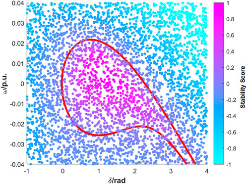
FIGURE 4. Stability Scores of the SIMB system samples.

4 Case study

The IEEE New England test system is used as the base case of the TSA task. The parameters of the test system are taken from (Zheng et al., 2018). A three-phase short circuit to ground fault happened at the start and end sides of the 36 transmission lines used in the time- domain simulation. A total of 5,000 samples were generated and 80% of the samples were used for training, with 2,697 stable and 2,303 unstable. The input dataset contains 170 features, including the active and reactive power of the transmission lines, as well as the magnitudes and angles of the bus voltages. We would like to know if the Sample Significance Index is suitable for a variety of deep neural network structures, so, we compare the performance of the SSI in the three most popular deep learning models used in TSA, including the MLP, the convolutional neural networks (CNN), and the long short-term memory (LSTM). The structures of the models mentioned are given in Table 1.

TABLE 1

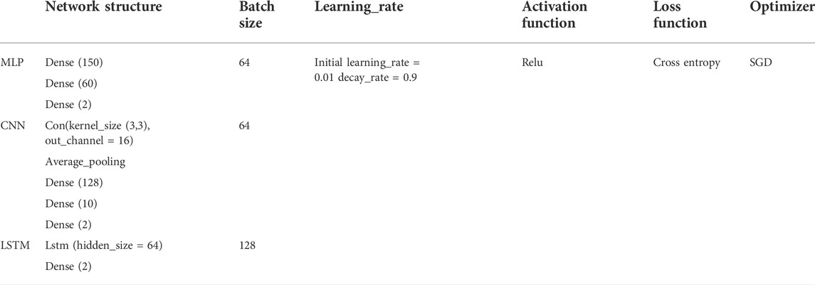
TABLE 1. Network structure and hyperparameters.

4.1 Dataset pruning

The average SSI used to prune the dataset is calculated by training the three networks on the full dataset for 10 training runs which are performed with 200 epochs. By various experiments, we find that the SSI becomes stable after 80 epochs, which is used as the Sample Significance Index. Then, the samples with low significance indexes are removed from the training, and a new model is trained with the same network using random initializing weights. The performance of the new model is computed using the testing set, shown in the blue lines of Figure 5. The red dashed line denotes the testing accuracy with random removal of the training samples, which decreases quickly as the fraction of the dataset pruning increases. However, with 50% of the low significance index samples pruned, the accuracy of each network is relatively stable, which is competitive with that using the full dataset. The results could help us to find the appropriate range of the dataset pruning without affecting the test accuracy.

FIGURE 5

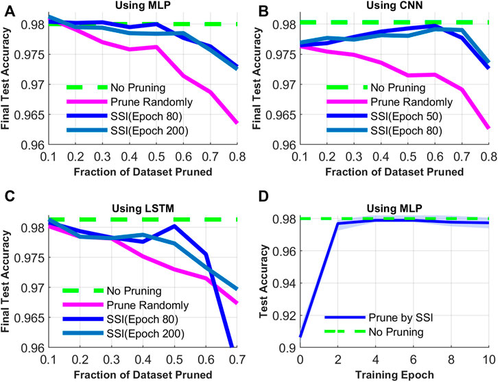
FIGURE 5. The influence of the pruning fraction and SSI of different training periods on the final accuracy. (A) to (C) show the test accuracy with different fractions of datasets pruned and pruning strategies using MLP, CNN, and LSTM. (D) shows the test accuracy of MLP using different SSI from different training epochs.

In the meantime, the performance in the accuracy of the subsets pruned on epoch80 and epoch200 indexes is similar. To investigate how early the SSI are effective in training, Figure 5D shows the training on a fixed number of samples (40%) selected by the SSI of early periods. Though the accuracy fluctuates at the first few epochs, the results suggest that early in the training, the average Sample Significance Index can identify samples that the deep network heavily uses to shape the decision boundary throughout the whole training process.

The loss is recorded when training the CNN using the full dataset and the subset pruned 50% samples based on SSI to explore the influence of pruning samples on the training dynamic process. And the loss surface called loss landscape is drawn along two directions from a center point, as shown in Figure 6. The surface figures and contour maps on the top and bottom rows show that the loss landscape of the subset is flatter than the full dataset. The flatter the loss landscape, the better the performance and generalization (Li et al., 2018).

FIGURE 6

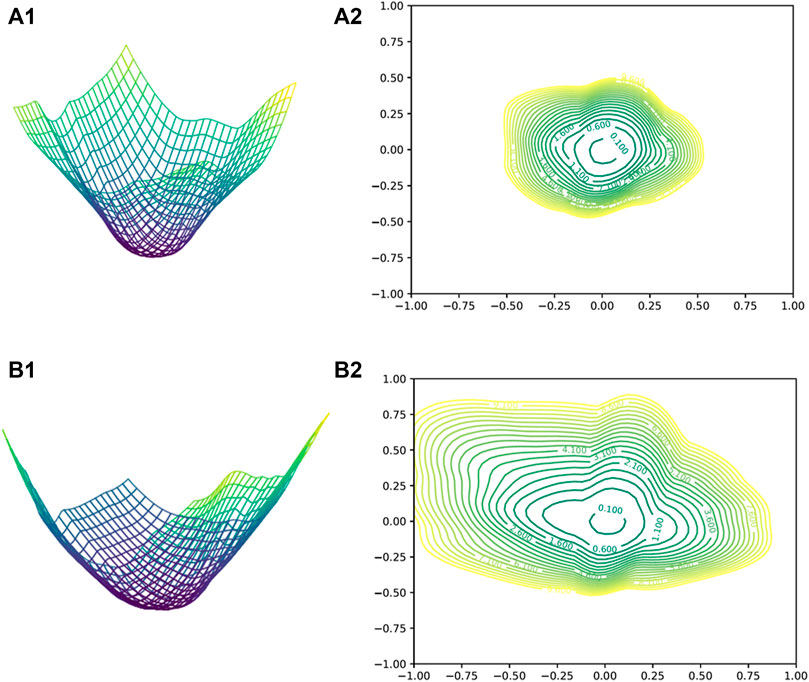
FIGURE 6. Loss landscape visualizations of CNN trained with the full dataset (A1,A2) and the subset with 50% samples of the full dataset (B1,B2). Left: The surface of the loss landscape. Right: The contour map of the loss landscape, loss = 10.

Table 2 records the time training subsets with different sizes take and the efficiency measured by the accuracy divided by the time. On one hand, with the size of a batch fixed, the number of mini-batches and total training time decreases, however, there is no significant decline in accuracy. On the other hand, the subsets selected by SSI at the early training period could get high accuracy, so the using of early period SSI is time-saving and reliable. On the whole, the use of SSI reduces dataset generation time and training time.

TABLE 2

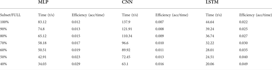
TABLE 2. Time and Efficiency of subsets with different sizes.

4.2 Samples with high SSI

In the study of 4.1, the samples with high SSI played an important role in TSA. In order to study the influence of the range of the Sample Significance Index on stability assessment accuracy, the key is to analyze whether the samples with the highest indexes have the highest accuracy. We first sort the samples by ascending SSI. Then, we perform a sliding window analysis on these samples by training on a subset of which the SSI of the samples within the window is from percentile p to percentile p+40%. And the step of window sliding to higher SSI is 10% of the full dataset. In three networks, the results indicate that the performance increases as the window slides to higher percentiles, as shown in Figure 7.

FIGURE 7

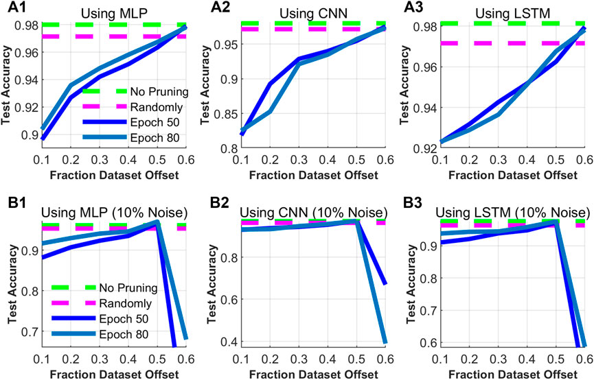
FIGURE 7. Test accuracy of MLP, CNN, and LSTM trained on the full dataset (No pruning) and a 40% subset pruned randomly or by SSI calculated at epoch 50 or epoch 80. When using SSI, the sample window slides along the samples in the ascending order of SSI. Training of the first row (A1–A3) uses the original dataset. In the second row (B1–B3), the dataset contains 10% randomized labels.

Since the sliding window contains 40% samples of the dataset, as shown in Figure 7, the samples with the highest SSI only account for 10% of the dataset. Rarely appearing in practical applications except for studying extreme cases, we use the sliding window which includes 10% of the total samples. The accuracy of the subsets increases as the sliding window moves to the high SSI region as shown in Figure 8. Not until the large part of the sliding window is in the highest index region will the MLP classification performance drop sharply. As the definition of SSI, the subset of the highest indexes includes the samples which are most prone to be misjudged in the process of TSA. Only using these samples, it is detrimental to integrally describe the decision boundary.

FIGURE 8

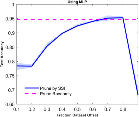
FIGURE 8. Test accuracy of MLP trained on only 10% subset which slides along the samples in the ascending order of SSI.

In the process of training dataset generation, the stability labels of some samples are generated incorrectly due to the selection of transient stability criteria or errors in the calculation. These labels can be regarded as noisy labels which could affect the accuracy of the networks and sample SSI calculation. Therefore, 10% sample labels of the dataset are randomly selected for randomization. Subsets containing 40% samples of this dataset are generated for training. As Figures 7B1–B3 show, in the same way, the accuracy drops sharply after reaching a peak. Furthermore, Figure 9 shows the distribution of the stability labels sorted by SSI from small to large along the axis which explains the sharp drop. The samples with randomized labels congregate in the highest SSI region, which greatly interferes with the accuracy of the model training.

FIGURE 9

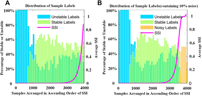
FIGURE 9. Distribution of stability labels and SSI. The dataset of (A) is the original full dataset and (B) contains 10% noisy labels. All samples are arranged in the ascending order of SSI. The minimum scale on the x-axis is 100 and the average SSI is calculated from 100 samples.

This part indicates that a set number of samples with higher SSI do not necessarily mean higher accuracy. And it may influence the formation of the decision boundary in the opposite way. And a fixed-length sliding window of the samples along the SSI provides us with an intuitive way to generate datasets which will be discussed in the next part.

4.3 Implications for dataset generation

In addition to the samples with high SSI that we care about, an interesting phenomenon, as shown in Figure 9, is that regardless of the existence of the noise, unstable samples make up a larger proportion in low SSI regions than stable samples. Mainly because the input features such as the voltage and power angles are prone to oscillation and divergence after the instability of the power system. So, the unstable samples could be accurately identified by a network than stable samples in the TSA task. In other words, samples with high or even medium SSI participating in the formation of the stability boundary is beneficial to get the higher accuracy and better generalization performance.

What’s more inspired by the results of the SMIB system, we evaluate the relations between the SSI and the critical-clearing time, as shown in Figure 10. The CCT is computed by a binary search method numerically for each fault. Each point indicates a sample used in the training set. The trend is clear that the closer the clearing time is to the CCT, the larger the SSI is. Since the relative clearing time is highly related to the stability boundary and the sample significance is related to the decision boundary, it is straightforward to conclude that the physical interpretation of the decision learned is the stability boundary of the system. Figure 10 also implies that generating the samples close to the stability boundary is a more efficient dataset-construction method.

FIGURE 10

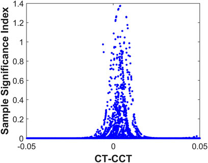
FIGURE 10. Sample Significance Index distribution with relative clearing time.

5 Conclusion

In summary, this article evaluates the significance of the samples for the deep learning-based TSA. It is observed that a large amount of samples can be pruned at an early training stage without sacrificing test accuracy using the Sample Significance Index. In addition, we find that the samples with high significance scores tend to have a borderline fault-clearing time. This is intuitive. The samples with short or long fault-clearing times can be regarded as the white and black samples. It is always easy to separate the whites from the blacks. But the samples with borderline fault clearing times are “gray” samples, which are more important for learning the stability boundary and improving the training accuracy. Therefore, this article proposes a method to generate and prune the dataset based on the Sample Significance Index for TSA which provides some relief to data generation and training. And combining the stability score and the classification results of the networks, we get a more intuitive method to assess the transient stability of samples.

Future work includes how we can use SSI to understand the dynamic training process of models since we have already known the early training period and final results. More tests on datasets and power system topologies are also preferred to show the properties of the significance index. Ultimately, we want the SSI to be a part of the tool to generate and evaluate some benchmark datasets for power system TSA analyses so that various algorithms can be tested in a unified and standard platform like computer vision or natural language-processing fields.

Data availability statement

The original contributions presented in the study are included in the article/Supplementary Material;further inquiries can be directed to the corresponding author.

Author contributions

LZ: inspiration of algorithm, data analysis, manuscript writing, and reviewing. ZW: experiment implementation, manuscript reviewing, and editing. GL: supervision. YX: supervision.

Funding

This work was supported in part by the National Key R&D Program of China “Response-driven intelligent enhanced analysis and control for bulk power system stability” (2021YFB2400800).

Conflict of interest

The authors declare that the research was conducted in the absence of any commercial or financial relationships that could be construed as a potential conflict of interest.

Publisher’s note

All claims expressed in this article are solely those of the authors and do not necessarily represent those of their affiliated organizations, or those of the publisher, the editors, and the reviewers. Any product that may be evaluated in this article, or claim that may be made by its manufacturer, is not guaranteed or endorsed by the publisher.

Supplementary material

The Supplementary Material for this article can be found online at: https://www.frontiersin.org/articles/10.3389/fenrg.2022.925126/full#supplementary-material

References

Azman, S. K., Isbeih, Y. J., El Moursi, M. S., and Elbassioni, K. (2020). A unified online deep learning prediction model for small signal and transient stability. IEEE Trans. Power Syst. 35 (6), 4585–4598. doi:10.1109/TPWRS.2020.2999102

CrossRef Full Text | Google Scholar

Campbell, T., and Broderick, T. (2018). “Bayesian coreset construction via greedy iterative geodesic ascent,” in 35th International Conference on Machine Learning, ICML 2018, Stockholm, Sweden, July 10–15, 2018, 698–706.

Google Scholar

Hagmar, H., Tong, L., Eriksson, R., and Tuan, L. A. (2021). Voltage instability prediction using a deep recurrent neural network. IEEE Trans. Power Syst. 36 (1), 17–27. doi:10.1109/TPWRS.2020.3008801

CrossRef Full Text | Google Scholar

Hwang, M., Jeong, Y., and Sung, W. (2020). “Data distribution search to select core-set for machine learning,” in ACM International Conference Proceedings Series, Utrecht, Netherlands, October 25–29, 2020, 17–19. doi:10.1145/3426020.3426066

CrossRef Full Text | Google Scholar

Kundur, P. (1994). Power system stability and control. New York, NY, USA: McGraw-Hill.

Google Scholar

Li, H., Xu, Z., Taylor, G., Studer, C., and Goldstein, T. (2018). “Visualizing the loss landscape of neural nets,” in Advances in neural information processing systems, 6389–6399.

Google Scholar

Paul, M., Ganguli, S., and Dziugaite, G. K. (2021). “Deep learning on a data diet: Finding important examples early in training,” in Advances in neural information processing systems 34, 20596–20607.

Google Scholar

Shi, Z., Yao, W., Zeng, L., Wen, J., Fang, J., Ai, X., et al. (2020). Convolutional neural network-based power system transient stability assessment and instability mode prediction. Appl. Energy 263, 114586. doi:10.1016/j.apenergy.2020.114586

CrossRef Full Text | Google Scholar

Sulistiawati, I. B., Priyadi, A., Qudsi, O. A., Soeprijanto, A., and Yorino, N. (2016). Critical Clearing Time prediction within various loads for transient stability assessment by means of the Extreme Learning Machine method. Int. J. Electr. Power & Energy Syst. 77, 345–352. doi:10.1016/j.ijepes.2015.11.034

CrossRef Full Text | Google Scholar

Sun, L., Bai, J., Zhou, Z., and Zhao, C. (2020). Transient stability assessment of power system based on Bi-directional long-short-term memory network. Dianli Xit. Zidonghua/Automation Electr. Power Syst. 44 (13), 64–72. doi:10.7500/AEPS20191225003

CrossRef Full Text | Google Scholar

Toneva, M., Trischler, A., Sordoni, A., Bengio, Y., Des Combes, R. T., and Gordon, G. J. (2019). “An empirical study of example forgetting during deep neural network learning,” in 7th International Conference on Learning Representations, ICLR 2019, New Orleans, USA, May 6–9, 2019.

Google Scholar

Wu, S., Zheng, L., Hu, W., Yu, R., and Liu, B. (2020). Improved deep belief network and model interpretation method for power system transient stability assessment. J. Mod. Power Syst. Clean Energy 8 (1), 27–37. doi:10.35833/MPCE.2019.000058

CrossRef Full Text | Google Scholar

Yang, D., Ji, M., Zhou, B., Bu, S., and Hu, B. (2021). Transient stability assessment of power system based on DGL-GAN. Dianwang Jishu/Power Syst. Technol. 45 (8), 2394–2945. doi:10.13335/j.1000-3673.pst.2020.1066

CrossRef Full Text | Google Scholar

Zheng, L., Hu, W., Zhou, Y., Min, Y., Xu, X., Wang, C., et al. (2018). “Deep belief network based nonlinear representation learning for transient stability assessment,” in IEEE Power and Energy Society General Meeting, Portland, USA, August 5–10, 2018, 1–5. doi:10.1109/PESGM.2017.8274126

CrossRef Full Text | Google Scholar

Zhou, Z., Bu, G., Ma, S., Wang, G., Shao, D., Xu, Y., et al. (2021). Assessment and optimization of power system transient stability based on feature-separated neural networks. Dianwang Jishu/Power Syst. Technol. 45 (9), 3658–3667. doi:10.13335/j.1000-3673.pst.2020.1356

CrossRef Full Text | Google Scholar

Zhu, L., Hill, D. J., and Lu, C. (2020). Hierarchical deep learning machine for power system online transient stability prediction. IEEE Trans. Power Syst. 263 (3), 2399–2411. doi:10.1109/TPWRS.2019.2957377

CrossRef Full Text | Google Scholar