Interval Prediction Method for Wind Speed Based on ARQEA Optimized by Beta Distribution and SWLSTM

1 Introduction

Wind power generation differs from traditional fossil power generation methods. The integration of wind power into a power grid is restricted by the uncertainty and intermittency of wind speed. Therefore, to maximize the use rate of wind power, more accurate wind speed prediction is crucial for the control strategy of wind farms (Li et al., 2019; Naik et al., 2019; Li et al., 2020; Gan et al., 2021). This process can simultaneously deal with the indetermination of wind farms and decrease the schedule deflection of power systems (Zhang YX. et al., 2016; Liang et al., 2017; Khosravi et al., 2018; Wang and Li, 2018). A precise wind speed prediction interval (PI) can assist policymakers to control deviations in transmission network planning and dispatching, risk evaluation, and reliability estimation. It is also a key factor to be considered in reducing peak loads, guaranteeing backup capacity, and increasing the safe performance of large-scale wind power generation systems (Wang et al., 2016).

In general, wind speed prediction methods can be divided into two types: point wind speed prediction (PWS) and PI of wind speed (PIWS). Compared with PWS, PIWS can obtain additional upper and lower bounds for the predicted wind speed, which can provide more predictive information. Traditional PWS methods include physical, statistical, and artificial intelligence models. A PWS prediction method is simple in construction and facile to implement in wind farms. However, it is usually difficult to obtain accurate prediction results with this method because of the randomness and intermittent nature of wind resources. Although a lot of studies focus on improving the preciseness of the PWS method and have made some progress, the impact of wind power uncertainty still cannot be solved. For instance, the inhomogeneous distribution of wind farms is affected by local terrain, the nonlinear vibration of wind generators, and machine halts outside the plan (Kiplangat et al., 2016; Li and Jin, 2018; Wang et al., 2018). Therefore, errors occur in wind power prediction, posing risks to grid dispatch. By contrast, PIWS can provide additional forecast information and reduce risks in grid dispatch (Yuan et al., 2017a; Peng et al., 2017); thus, it will improve the understanding of decision-makers on the indeterminacy of wind power fluctuations to avoid potential risks.

In recent years, many studies were conducted on the uncertainties of wind power generation, and PIWS has already been used for many actual items. There are two sorts divisions of the PIWS methods. The first one uses neural networks to directly obtain the upper and lower bounds of PIs. As an instance, the lower bound/upper bound estimation (LUBE) for forecasting wind speed time series is a significant breakthrough in PIWS (Zhang et al., 2016b). The method solves the problem of probability prediction by constructing PIs, wherein an interval is represented by upper and lower estimates. However, the LUBE cannot deal with the fluctuation as an indetermination in wind speed time series. Another interval prediction method involves estimating PIs on the basis of the probability density of a point prediction result. To determine the uncertainty of wind speed, it is necessary to construct the probability density curve of prediction results, which requires the probability density prediction method. This can provide accurate prediction information on power system operation through this curve.

The preciseness of the wind speed probability distribution function (PDF) is determined by the selected approaches and the prediction error level, because the key factor of PIWS estimation is the PDF of forecasting error (Allen et al., 2017; Naik et al., 2018; Zhao et al., 2018). A shared weight long short-term memory (SWLSTM) neural network can decrease the variable number that should be optimized (Zhang et al., 2019). It also exhibits the advantages of nonlinear prediction, fast convergence, and the capability to capture the long-term correlations of the time series. At present, the SWLSTM model has been applied for wind speed prediction. Previous studies have shown that wind speed time series demonstrate long-term memory characteristics. The present study adopts the SWLSTM model as the basis for wind speed prediction. In addition, normal or Laplace distribution functions and beta distribution functions are also widely used as PDFs in the field of PIWS. Among them, the beta distribution is more effective in estimating the PIWS than the normal distribution and Laplace distribution (Ren et al., 2016). The beta distribution is selected as the basis of the PIWS in the present study consequently.

In this study, to improve the accuracy of wind speed, a new hybrid method based on the SWLSTM model and beta–ARQEA algorithm is proposed, which combines methods of artificial intelligence and statistics. The main contributions are listed as follows in four parts:

1) The SWLSTM model is applied to wind speed prediction. The partial autocorrelation function is adopted to determine the input variables of the SWLSTM model to reduce the prediction error.

2) The real-coded quantum evolutionary algorithm (ARQEA) of alleles (Zhang et al., 2016c) is adopted to optimize the shape and position parameters in the beta distribution function for selecting the appropriate distribution function to fit the wind speed prediction error obtained by the SWLSTM model.

3) The entire wind speed time series are divided into plenty of intervals per error distribution to improve the prediction accuracy of PIWS methods.

4) The optimized parameters of different distribution functions are utilized to fit the prediction error of each wind speed interval, then confirm the confidence interval of the wind speed series, and superimpose them to get the PI of the entire wind speed. The PIWS based on beta–ARQEA–SWLSTM achieves higher reliability and narrower interval bandwidth.

Eventually, the PI of the entire wind speed series is acquired by superimposing the confidence interval of each wind speed level. Therefore, the PIWS based on beta–ARQEA–SWLSTM achieves higher reliability and narrower interval bandwidth.

The rest part of this study is as follows: a review of the principle of an SWLSTM neural network is shown in Section 2. Section 3 presents the key theory of ARQEA optimization parameters based on beta distribution and discusses how to use it to calculate confidence intervals. The PIWS process with the beta–ARQEA−SWLSTM model is introduced in section 4. Section 5 contains a case study and result analysis. Section 6 provides the conclusion drawn from the study.

2 SWLSTM Neural Network

The SWLSTM model is a special artificial intelligence model. It keeps the characteristics of the recurrent neural network model, which can make use of a series of memory cells to deal with the arbitrary input data and enhance the learning process of the time series. In addition, the SWLSTM model can capture the long-term dependence of the input data to prevent the gradient disappearing from information transmission, which enhances its capacity to capture the dynamic changes of the time series.

In SWLSTM, a new type of shared gate is proposed, which is composed of input, output, and forget gate. The network structure is shown in Figure 1. SWLSTM does not change the gate structure of the standard long short-term memory (LSTM), but shares the weight and bias of the gate structure. The advantages of SWLSTM are reducing the number of variables that must be optimized and shortening the training time (Zhang et al., 2019).

FIGURE 1

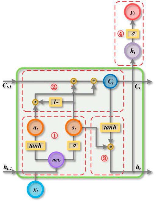
FIGURE 1. Schematic of the SWLSTM network structure.

As shown in Figure 1, the shared gate in the SWLSTM model has an inherent relationship with the time series, of which the purpose is to ensure that the training results often tend to be the new input information. Hence, training the time series model by the SWLSTM model has some advantages.

The hyperparameters of the SWLSTM model are shown in Table 1.

TABLE 1

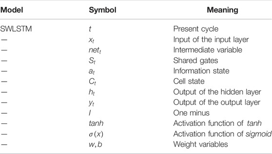
TABLE 1. Hyperparameters of the SWLSTM model.

In Figure 1, $x_t$ is the input of the input layer in the t-th cycle, $ne{t}_t$ is the intermediate variable in the t-th cycle, $S_t$ is the shared gates in the t-th cycle, $a_t$ is the information state in the t-th cycle, $C_t$ is the cell state in the t-th cycle, $h_t$ is the output of the hidden layer in the t-th cycle, $y_t$ is the output of the output layer in the t-th cycle, $I-$ is one minus, and $tanh,\sigma$ is the activation function.

SWLSTM has two stages: forward propagation and back-propagation. The process of forward propagation of SWLSTM in the tth cycle is discussed as follows.

1) Calculate the shared gate state and calculate the information gate state:

$ne{t}_t=w_h\cdot h_{t-1}+w_x\cdot x_t+b,(1)$

$S_t=\sigma \left(ne{t}_t\right)=\sigma \left(w_h\cdot h_{t-1}+w_x\cdot x_t+b\right),(2)$

$a_t=\text{tanh}\left(ne{t}_t\right)=\text{tanh}\left(w_h\cdot h_{t-1}+w_x\cdot x_t+b\right).(3)$

2) Update the cell state:

$C_t=s_t\ast C_{t-1}+\left(1-s_t\right)\ast a_t.(4)$

3) Calculate the output of the hidden layer:

$h_t=s_t\ast \text{tanh}\left(C_t\right).(5)$

4) Output predicted value of the output layer:

$y_t=s\left(z_t\right)=\sigma \left(w_y\cdot h_t+b_y\right).(6)$

In the preceding formula and figure, t represents the current cycle, $x_t$ is the input of the input layer, $S_t$ is the shared gates, and $a_t$ is the information state. $C_{t-1}$ and $C_t$ represent the cell state in the previous and current cycles, respectively. $h_{t-1}$ and $h_t$ denote the output of the hidden layer in the previous and current cycles, respectively. $y_t$ is the forecasted value of the current cycle. Intermediate variables are represented by $ne{t}_t$ and $z_t$. $\left[w_h,w_x,b\right]$ and $\left[w_y,b_y\right]$ are two sets of weight variables that must be optimized. Symbol $\cdot$ and $\text{∗}$ indicate matrix multiplication and multiplication between matrix elements, respectively. $\sigma \left(x\right)$ is the activation function of sigmoid and $tanh\left(x\right)$ is the activation function of tanh.

The process of error back-propagation in the tth cycle of the SWLSTM is discussed as follows.

1) Use the squared error function as the optimization objective:

$Et=\frac{1}{2}{\left(y_t-Y_t\right)}^2.(7)$

2) Calculate the error of variables in the output layer:

$\delta y_t=\frac{\partial E_t}{\partial y_t}=y_t-Y_t,(8)$

$\delta z_t=\frac{\partial E_t}{\partial z_t}=\frac{\partial E_t}{\partial y_t}\frac{\partial y_t}{\partial z_t}=\delta y_t\ast \left[y_t\ast \left(1-y_t\right)\right],(9)$

$\delta w_y=\frac{\partial E_t}{\partial w_y}=\frac{\partial E_t}{\partial z_t}\frac{\partial z_t}{\partial w_y}=\delta z_t\cdot h_t,(10)$

$\delta b_y=\frac{\partial E_t}{\partial b_y}=\frac{\partial E_t}{\partial z_t}\frac{\partial z_t}{\partial b_y}=\delta z_t\cdot 1=\delta z_t.(11)$

3) Calculate the error of variables in the hidden layer:

$\delta h_t=\frac{\partial E_t}{\partial h_t}=\{\begin{array}{c}\frac{\partial E_t}{\partial z_t}\frac{\partial z_t}{\partial h_t}=\delta z_t\cdot w_y , t=T,\\ \frac{\partial E_t}{\partial z_t}\frac{\partial z_t}{\partial h_t}+\frac{\partial E_t}{\partial ne{t}_{t+1}}\frac{\partial ne{t}_{t+1}}{\partial h_t}=\delta z_t\cdot w_y+\delta ne{t}_{t+1}\cdot w_h, t\ne T,\end{array}(12)$

$\delta C_t=\frac{\partial E_t}{\partial C_t}=\{\begin{array}{c}\frac{\partial E_t}{\partial h_t}\frac{\partial h_t}{\partial C_t}=\delta h_t\ast s_t\ast \left[1-{\text{tanh}}^2\left(C_t\right)\right], t=T,\\ \frac{\partial E_t}{\partial h_t}\frac{\partial h_t}{\partial C_t}+\frac{\partial E_t}{\partial C_{t+1}}\frac{\partial C_{t+1}}{\partial C_t}=\delta h_t\ast s_t\ast \left[1-{\text{tanh}}^2\left(C_t\right)\right]+\delta C_{t+1}\cdot s_t, t\ne T.\end{array}(13)$

The shared gates in SWLSTM reserve the functions of the three gates in the LSTM and still have the ability to discard useless historical information and keep current useful information. Coupling the input and forget gates simplified the LSTM without significantly decreasing the performance. Activation functions Sigmoid and tanh are retained in the SWLSTM. These two points indicate that the SWLSTM does not significantly reduce the prediction accuracy.

3 Estimation of Random Samples Based on the Beta–ARQEA Model

Considering the optimization problem of probability density function parameters in interval prediction methods, to find the appropriate distribution function for fitting prediction errors of wind speed obtained by the SWLSTM model, the present study uses random sample estimation based on the beta–ARQEA model. The position parameters in the beta distribution function are optimized by using ARQEA. The beta distribution is expressed for a random sample $R=\left\{r_1,r_2,\dots ,r_n\right\}$ as follows:

$\beta \left(\gamma ,\eta \right)=\underset{0}{\overset{1}{{\displaystyle \int }}}{z}^{\gamma -1}{\left(1-z\right)}^{\eta -1}dz,(14)$

where $\gamma >0, \eta >0$. $z=\left(r-a\right)/\left(b-a\right)$, where a and b are the position parameters of the beta distribution (Yuan et al., 2019). The PDF based on beta distribution can be expressed as $Y = f\left(R, \gamma , \eta , a, b\right)$, $n=1,2,\dots$.

Using ARQEA to find the optimal parameters of the beta distribution function can further improve the precision of the beta distribution model.

Allele real-coding for beta position parameters is as follows (Zhang YX. et al., 2016):

$\left|\begin{array}{c}\begin{array}{cc}positionparamete{r}_1& position paramete{r}_2\end{array}\\ \begin{array}{cc}positionparamete{r}_1^{\prime }& position paramete{r}_2^{\prime }\end{array}\end{array}\right|,(15)$

where $positionparamete{r}_i$ and $\mathit{position paramete}{\mathit{r}}_{\mathit{i}}^{\prime }$ are encoded in the form of probability stacking. This process can effectively increase population diversity, prevent the occurrence of premature phenomena, and provide preconditions for improving optimization. The relative superiority of $\mathit{position}\mathit{paramete}{\mathit{r}}_{\mathit{i}}$ and $\mathit{position paramete}{\mathit{r}}_{\mathit{i}}^{\prime }$ is determined in accordance with the distance relationship between each iteration process and the present optimal solution. The one that is closer to the present optimal solution is called the “better gene” $x_i$, and the other is called the “poor gene” $x_i^{\prime }$. The hybrid evolution strategy is adopted to balance the global search and local search for different advantages.

1) The “better gene” $x_i$ fully uses existing information to approach the present optimal solution under the guidance of the present optimal solution while searching for a better solution, which is

$x_{inew}=x_i+sign\left(x_i^{\ast }-x_i\right)\cdot \left(K\left|x_i^{\ast }-x_i\right|\right),(16)$

where $sign(x_i^{\ast }-x_i)$ controls the evolution direction, K is the set constant that controls the step length of the directional evolution, and $\left|x_i^{\ast }-x_i\right|$ is the maximum range of evolution.

2) For the “poor gene” $x_i^{,}$ , a local search with a scale shrink is used, that is,

$x_{inew}=x_i+U\left(-\mathrm{1,1}\right)\cdot \left(1-\text{arctan}\left(\frac{r}{g}\right)\right)\cdot \Delta d,(17)$

where $U(-\mathrm{1,1})$ is a random distribution between −1 and 1; $r$ is the present algebra; $g$ is the maximum iteration algebra; $\left(1-\text{arctan}\left(\frac{r}{g}\right)\right)$ is the contraction function that decreases from 1 to 0 as algebra $r$ increases, causing the scale of variation to decrease gradually with evolution; and $\Delta d$ is the allowable range of variation.

The “better gene” and the “poor gene” perform local search and global search, respectively. A hybrid evolution strategy is developed when the two genes are transformed into each other, enhancing the balance between the local search and global search of the algorithm.

To evaluate the performance of the beta distribution model, the approximate index $I$ is selected, which is defined as follows:

$I=\frac{{{\displaystyle \sum }}_{n-1}^M{\left(y_n-{\overline{N}}_n\right)}^2}{M},y_n=f\left({\overline{C}}_n\right),n=\mathrm{1,2},\mathrm{...},M,(18)$

where $M$ is the number of frequency distribution histograms; in the nth histogram, ${\overline{N}}_n$ and ${\overline{C}}_n$ are the height and center position, respectively; the approximation PDF is represented as $f\left({\overline{C}}_n\right)$ ; and $y_n$ is the approximate PDF value of ${\overline{C}}_n$ center position. When the fitting index $I$ is small, approximation accuracy is high.

According to Eq. 18, the fitness function of the beta distribution optimization model and its constraints can be obtained as follows:

$\text{min}fitness=\text{min}\left(I\right),(19)$

$s.t.\{\begin{array}{c}\gamma ,\eta \in \left(\mathrm{0,1}\right),\\ a,b\in \left(x_{min},x_{max}\right),\end{array}(20)$

where $x_{min}$ and $x_{max}$ are the minimum and maximum values, respectively, of the sample.

To obtain the PDF of beta–ARQEA, we calculate the histogram of the frequency distribution of the sample $X=\left\{x_1,x_2,...,x_n\right\}$ to obtain the desired fitting objective, then randomly initialize the parameters $(a,b,\gamma ,\eta )$ of the beta distribution function according to the constraint (20). After that, calculate the distance of each position parameter, determine the better gene and poor gene, then calculate the fitness of the genes, and retain the genes with better fitness. When the maximum number of iterations is reached, stop the loop. Finally, obtain the optimal parameters $(a, b, \gamma , \eta )$ of the beta distribution function. According to Eq. 14, we can get the PDF based on optimized beta distribution.

After obtaining the PDF, the distribution function $F\left(x\right)$ can be calculated by integration, the definition of which is as follows:

$F\left(x\right)={\displaystyle \underset{0}{\overset{1}{\int }}\left(\text{PDF}\left(p\right)\right)dx}.(21)$

Presume the confidence level is $100(1-\alpha )\%$, and the unknown parameter for sample $X$ is $\theta$. If $P\{\theta 1<\theta <\theta 2\}= 1–\alpha$ and the interval $[\theta 1, \theta 2]$ is minimum, these two conditions are satisfied at the same time, and the interval $[\theta 1, \theta 2]$ occurs at a certain level of confidence, then

$\{\begin{array}{c}{\theta }_1=F\left(\frac{\alpha }{2}\right),\\ {\theta }_2=F\left(1-\frac{\alpha }{2}\right).\end{array}(22)$

Then, we can obtain the confidence interval $(\theta 1, \theta 2)$ of θ with the confidence level $100\times (1-\alpha )\%$.

4 PIWS Estimation Based on the Beta–ARQEA–SWLSTM Model

Since the SWLSTM’s point prediction accuracy is high and beta–ARQEA’s probability prediction results are reliable, SWLSTM and beta–ARQEA are combined to obtain high-precision point prediction, high-reliability interval prediction, and probability prediction. The wind speed PI implementation process based on the beta–ARQEA–SWLSTM model can be shown as follows:

Step 1: Divide the wind speed historical data into training dataset $Data1$ and test dataset $Data2$, $Data1 = \{x_1, x_2, \mathrm{...}, x_n\}$, $Data2 = \{ x_1, x_2, \mathrm{...}, x_n\}$.

Step 2: $Data1$ and $Data2$ are normalized, and new training data $X_1$ and new test data $X_2$ are obtained.

Step 3: The PACF of $X_1$ is calculated, and the lag coefficient with a value of $k$ is obtained. Then, the input data of the SWLSTM model are determined as follows: $input = \{x_{t-1}, x_{t-2}, \mathrm{...}, x_{t-k}\}$, where $t = (k, k+1, k+2, \mathrm{...}, m)$, $t\ge k$ , and $k>0$.

Step 4: $X_1$ is used to train the SWLSTM model, and the trained SWLSTM model is obtained.

Step 5: $X_2$ is used to test the trained SWLSTM model, and wind speed prediction $Y_2 = \{y_1, y_2, \mathrm{...}, y_n\}$ is determined.

Step 6: The errors between $X_2$ and $Y_2$ are calculated, and the error can be written as $D = \{d_1, d_2, \mathrm{...}, d_n\}$, where $d_i = y_i - x_i$ and $i = 1, 2, \mathrm{...}, n$.

Step 7: The predicted data $Y_2$ are divided into $K$ levels in accordance with the rated speed of a wind farm.

Step 8: Wind speed prediction values and their forecasting errors under each wind speed level are statistics. The values and errors are denoted as $Y_{2k}=\{y_1^k,y_2^k,\mathrm{...},y_{nk}^k\}$ and $D_k=\{d_1^k,d_2^k,\mathrm{...},d_{nk}^k\}$, where the prediction error number of the kth wind speed level is represented as $nk$.

Step 9: Input $D_k$ to the beta–ARQEA, and the upper-lower limits of every wind speed level are calculated according to Eq. 22. Then obtain the PI of the kth wind speed level $[{\Delta }_k^1,{\Delta }_k^u]$.

Step 10: The wind speed series PI of every level, which can be represented as $[Y_{2k}+{\Delta }_k^1,Y_{2k}+{\Delta }_k^u]$, is acquired.

Step 11: The entire wind speed series PI consists of each wind speed level.

Wind speed PI implementation based on the beta–ARQEA–SWLSTM is shown in Figure 2.

FIGURE 2

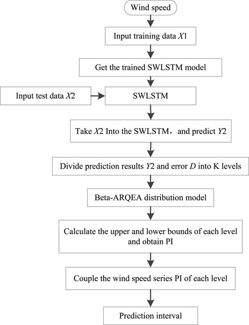
FIGURE 2. Wind speed PI implementation based on beta–ARQEA–SWLSTM.

5 Case Study

5.1 Wind Speed Series Data

In the current study, the wind speed series data of a wind farm in Jilin, China, are used. The wind speed series data in April 2018 were selected, which were measured and recorded by the wind tower. The step of wind speed series data is 15 min. The model of the wind turbine used in the wind farm is S82–1.5, the rated wind speed is 13 m/s, and the cut-in wind speed and the cut-out wind speed are 4 m/s and 20 m/s, respectively. To verify the performance of the model, four datasets are selected for testing, one of which is shown in Figure 3. Each dataset uses a data length of 7 days consisting of 672 wind speed time series. Take approximately 80% of the data from every set as a training set and take the remaining portion as a validation set. The training set is used to calibrate the parameters of the beta–ARQEA–SWLSTM model and the validation set is used to verify the performance of the beta–ARQEA–SWLSTM model for the prediction interval of wind speed.

FIGURE 3

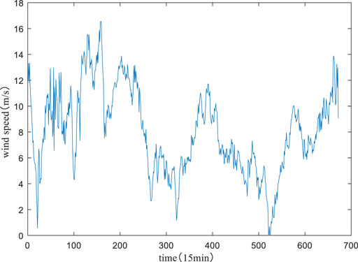
FIGURE 3. Dataset of wind speed.

5.2 Evaluation Criteria

5.2.1 Evaluation Criteria of PIWS

To evaluate the performance of different models, these indicators are selected to verify the effectiveness of the PI model: PI coverage probability ( $PICP$), average bandwidth ($\Delta \overline{P}$), index $F$, and sharpness (${\overline{S}}^{\alpha }$) (Yu et al., 2018).

To clarify the definition, the ith measured value is represented by $x_i$, and thus, $I\left(i\right)=[lb\left(i\right),ub\left(i\right)]$ represents the $100(1-\alpha )\%$ confidence PI of $x_i$, which is a random interval, where $lb\left(i\right)$ is the upper limit and $ub\left(i\right)$ is the lower limit. The $PICP$ is shown as follows:

$PICP=\frac{1}{n}{\displaystyle \sum }_{i=1}^n{c}_i,(23)$

where $n$ is the number of samples and $c_i$ is the indicator of $PICP$. If $X = 1$, then $c_i=1$; otherwise $c_i=0$.

The average bandwidth $\Delta \overline{P}$ is defined as:

$\{\begin{array}{c}\Delta \overline{P}=\frac{1}{n}{\displaystyle \sum }_{i=1}^n\Delta P_i,\\ \Delta P_i=ub\left(i\right)-lb\left(i\right).\end{array}(24)$

At the same confidence level, a smaller $\Delta \overline{P}$ results in better performance of the PI.

If the interval width $\Delta \overline{P}$ is narrower and $PICP$ is larger, there will be better prediction results. Therefore, we use a comprehensive index $F$, which considers $PICP$ and $\Delta \overline{P}$, to evaluate the performance of the PI (Tasnim et al., 2018):

$F=\frac{2\times PICP\times \frac{1}{\Delta \overline{P}}}{PICP+\frac{1}{\Delta \overline{P}}}, ifPICP\ge \left(1-\alpha \right).(25)$

The $F$ value takes into account two contradictory indicators, which can integrate the evaluation of the quality of the PI. The higher the $F$, the more effective the test method will be.

In accordance with the concept of sharpness, the quality of the PI opposite to $x_i$ can be computed, denoted by $S^{\alpha }\left(x_i\right)$, which is defined as

$S^{\alpha }\left(x_i\right)=\{\begin{array}{c}-2\alpha ·\Delta P_i-4\left[lb\left(i\right)-x\left(i\right)\right], if x\left(i\right)<lb\left(i\right),\\ -2\alpha ·\Delta P_i, if x\left(i\right)<l\left(i\right),\\ -2\alpha ·\Delta P_i-4\left[x\left(i\right)-ub\left(i\right)\right], if ub\left(i\right)<x\left(i\right).\end{array}(26)$

Here, sharpness ${\overline{S}}^{\alpha }$ is defined as

${\overline{S}}^{\alpha }=\frac{1}{n}\left|{\displaystyle \sum }_{i=1}^n{S}^{\alpha }\left(x_i\right)\right|.(27)$

Here, a smaller $S^{\alpha }\left(x_i\right)$ indicates higher PI quality.

5.2.2 Probability Prediction Evaluation Indicator

To verify the certainty, ensemble, and probability prediction, the comprehensive evaluation indicator of prediction performance, namely the continuous sorting probability score ($CRPS$) (Alessandrini et al., 2015), is adopted. Assuming that $p\left(y_i\right)$ is the PDF of the ith forecast value obtained by the beta–ARQEA–SWLSTM, $F\left(y_i\right)$ is the cumulative distribution function (CDF) of $p\left(y_i\right)$. The $CRPS$ is defined as

$CRPS=\frac{1}{Te}{\displaystyle \sum }_{i=1}^{Te}\underset{-\infty }{\overset{+\infty }{{\displaystyle \int }}}{\left[F\left(y_i\right)-H\left(y_i-Y_i\right)\right]}^{2}d{y}_i,(28)$

$F\left(y_i\right)=\underset{-\infty }{\overset{y_i}{{\displaystyle \int }}}p\left(x\right)dx,(29)$

$H\left(y_i-Y_i\right)=\{\begin{array}{cc}0,& y_i<Y_i,\\ 1,& others,\end{array}(30)$

where $H(y_i-Y_i)$ is the Heaviside function. When the $CRPS$ is smaller, the comprehensive performance is better.

5.2.3 Reliability Evaluation Indicator

Reliability is the statistical consistency between forecasting and observations. Probabilistic integral transformation ($PIT$) values are used to evaluate the reliability of forecasting by a unified probabilistic graph (Liu et al., 2018). $PIT$ is computed by observation results and CDF, which is defined as:

$PIT=F\left(Y_i\right)=\underset{-\infty }{\overset{Y_i}{{\displaystyle \int }}}p\left(x\right)dx.(31)$

To check whether the $PIT$ values of the test samples follow uniform distribution, all test samples can be found from the uniform probabilistic graph. $PIT$ values will be uniformly distributed between 0 and 1 if the forecast is reliable.

5.3 Results and Analysis

To verify the effectiveness of the method proposed in this research, beta–ARQEA–SWLSTM is compared with other wind speed prediction methods in terms of point prediction accuracy, PI suitability, and probability prediction comprehensive performance. Then, the reliability of beta–ARQEA–SWLSTM is verified.

1) Point prediction results of wind speed.

To test the point forecasting accuracy of the method, the beta–ARQEA–SWLSTM model is applied for wind speed forecasts. The results are shown in Figure 4.

FIGURE 4

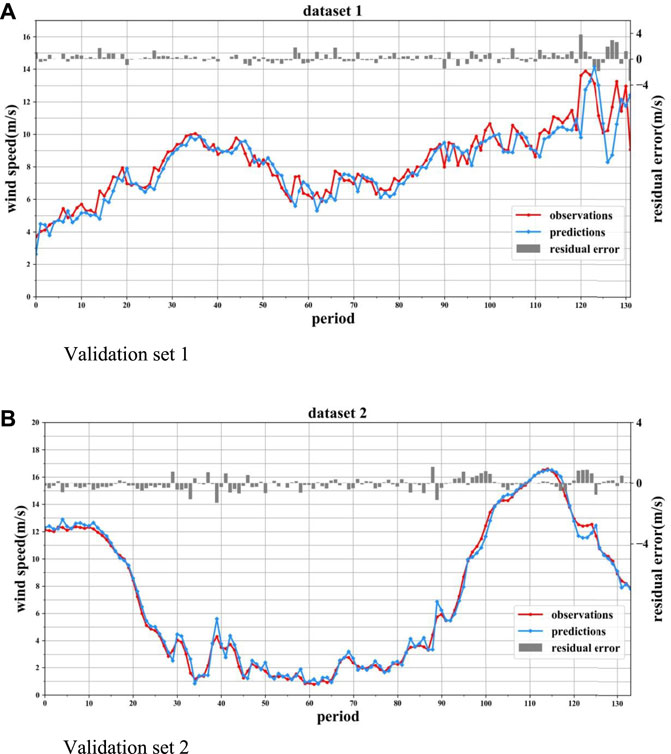
FIGURE 4. Wind speed prediction results for validation sets 1 and 2. (A) Validation set 1. (B) Validation set 2.

It can be seen from Figure 4 that the wind speed forecasted values of the SWLSTM model is near the observed values. The PDF is difficult to fit all the wind speed forecasting errors, so we partition the wind speed into 10 wind speed grades following the predicted value. The grade gap of wind speed is 0.1 $S$, in which $S$ is the cut-out wind speed. Compare the beta–particle swarm optimization (PSO)–SWLSTM model (beta–PSO–SWLSTM), standard beta distribution SWLSTM model (beta–SWLSTM), and least square support vector machine (LSSVM) model with the beta–ARQEA–SWLSTM model to verify the validity of the beta–ARQEA–SWLSTM model. In accordance with Eq. 19, the fitting indexes of these models are shown in Table 2.

TABLE 2

TABLE 2. Fitting indicators in each wind speed grade of the four models.

When the results of each distribution model in Table 2 are compared with that of the beta–ARQEA distribution model, the fitting indicator $I$ output by the beta–ARQEA model is the smallest among the four distribution models for every wind speed grade, indicating that the beta–ARQEA–SWLSTM model has the highest accuracy. This finding proves that the beta–ARQEA–SWLSTM model is superior to other models in wind speed point prediction.

2) Interval estimation of wind speed.

The interval estimation of wind speed is to verify the suitability of beta–ARQEA–SWLSTM. The wind speed PI results obtained from beta–ARQEA–SWLSTM are shown in Figure 5.

FIGURE 5

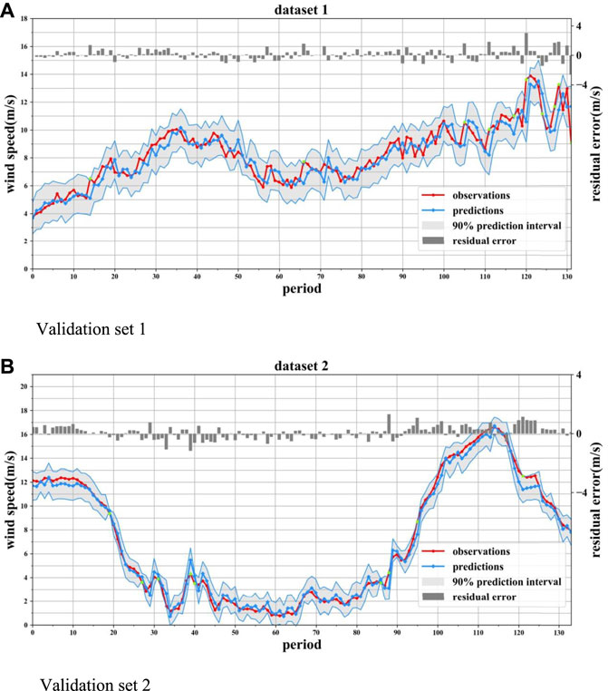
FIGURE 5. Wind speed PI at 90% confidence level. (A) Validation set 1. (B) Validation set 2.

It can be seen from Figure 5 that the PI adopting the beta–ARQEA–SWLSTM model basically contains all the actual wind speed data. The little green dots in Figure 5 are the points at which the observation exceeds the prediction interval of beta–AEQEA–SWLSTM. The performance indicators of four models are computed and compared to verify the superiority of the beta–ARQEA–SWLSTM model. The results are shown in Table 3.

TABLE 3

TABLE 3. Performance of the compared PIWS models.

As indicated in Table 3, the coverage rate of each model reached 90%. When the coverage rate reaches the standard, the interval width is represented by $\Delta \overline{P}$. In the four models, the beta–ARQEA–SWLSTM model has the smallest $\Delta \overline{P}$, the smallest sharpness ${\overline{S}}^{\alpha }$, and the highest $F$ index, indicating that the bandwidth of the wind speed PI obtained by the beta–ARQEA–SWLSTM model is narrower and has the highest sharpness and quality. In addition, there is a higher preference for PI. Based on the aforementioned results, it can be seen that the beta–ARQEA–SWLSTM model has a better coverage rate and narrow bandwidth in the wind speed PI, and can realize high-quality wind speed PI.

3) Probability prediction results.

To verify the entire performance of the PDF of each model, probability prediction evaluation is applied. The $CRPS$ is used to evaluate the whole PDF, and the results contain point forecast, PI, and the entire performance of the PDF (Tang et al., 2020; Zhang et al., 2020). The $CRPS$ of each model on each dataset is shown in Table 4. In each dataset, the $CRPS$ of beta–ARQEA–SWLSTM is optimal. This finding fits well with point prediction and PI.

4) Verification of beta–ARQEA–SWLSTM reliability.

TABLE 4

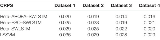
TABLE 4. Probability prediction metrics in each dataset.

To guarantee that the prediction results of beta–ARQEA–SWLSTM are convincing, the reliability evaluation is essential. If the prediction results are reliable, then the $PIT$ of each predicted value in the validation set should satisfy uniform distribution (Liu et al., 2018). To see the distribution of $PIT$ values intuitively, their uniform probability diagram is plotted, as shown in Figure 6.

FIGURE 6

FIGURE 6. Reliability test of beta–ARQEA–SWLSTM. (A) Validation set 1. (B) Validation set 2.

As can be seen from Figure 6, the $PIT$ range of the two datasets is uniformly covered (0,1), and uniformly distributed along the diagonal and at the Kolmogorov 5% visibility band, showing that the predicted PDF is in an appropriate range (Yuan et al., 2017b). In consequence, the prediction results of beta–ARQEA–SWLSTM are persuasive and reliable.

To summarize, compared with other models, the proposed hybrid model has higher accuracy, coverage rate and reliability in wind speed point prediction, interval estimation, probability prediction and reliability evaluation, and can provide higher quality wind speed prediction interval and more accurate results.

6 Conclusion

To achieve the goal of “carbon peaking, carbon neutralization,” clean and renewable wind energy is very important. Accurate wind speed prediction is crucial for the smooth operation of wind turbines and improving their connection to grids. A new hybrid method based on the ARQEA algorithm and beta–SWLSTM model is proposed to improve the accuracy of wind speed prediction and the convergence speed. Compared with the traditional PIWS method, the hybrid model retains functionality while being able to capture the long-term correlations of the time series. The intervals of the wind speed time series are divided by the error distribution, which enables the hybrid model to obtain a PDF with higher reliability and narrower interval bandwidth.

The proposed method is applied on a wind farm in Jilin, China, to verify its effectiveness on wind speed forecasting. In order to accurately verify the applicability of point prediction, interval prediction, and the reliability of probability prediction, six reference indexes of $PICP$, $\Delta \overline{P}$, ${\overline{S}}^{\alpha }$, $F$, $CRPS$, and $PIT$ are adopted. Compared with the results of other models, it can be seen that the beta–ARQEA–SWLSTM model can obtain a wider coverage range and narrower interval bandwidth. Moreover, the prediction results can also show high performance in point prediction, interval prediction, and probability prediction. The proposed method can not only be used for wind speed prediction problems but also for other problems related to time series.

The beta distribution is considered in the proposed model. However, for the wind power prediction problem, other distributions such as the Gaussian distribution may have a better performance for different scenarios. In future, more wind farms in different geographical conditions and more probability distribution hypotheses will be testified.

Data Availability Statement

The original contributions presented in the study are included in the article/Supplementary Material; further inquiries can be directed to the corresponding author.

Author Contributions

ZS was responsible for the specific work of this manuscript. XQ and YS carried out some of the calculation work. ZC and YT guided the work of this manuscript.

Funding

The authors acknowledge the funding of the National Key Research and Development Plan (2017YFB0902100).

Conflict of Interest

The authors declare that the research was conducted in the absence of any commercial or financial relationships that could be construed as a potential conflict of interest.

Publisher’s Note

All claims expressed in this article are solely those of the authors and do not necessarily represent those of their affiliated organizations, or those of the publisher, the editors, and the reviewers. Any product that may be evaluated in this article, or claim that may be made by its manufacturer, is not guaranteed or endorsed by the publisher.

References

Alessandrini, S., Delle Monache, L., Sperati, S., and Cervone, G. (2015). An Analog Ensemble for Short-Term Probabilistic Solar Power Forecast. Appl. Energy 157, 95–110. doi:10.1016/j.apenergy.2015.08.011

CrossRef Full Text | Google Scholar

Allen, D. J., Tomlin, A. S., Bale, C. S. E., Skea, A., Vosper, S., and Gallani, M. L. (2017). A Boundary Layer Scaling Technique for Estimating Near-Surface Wind Energy Using Numerical Weather Prediction and Wind Map Data. Appl. Energy 208, 1246–1257. doi:10.1016/j.apenergy.2017.09.029

CrossRef Full Text | Google Scholar

Gan, Z., Li, C., Zhou, J., and Tang, G. (2021). Temporal Convolutional Networks Interval Prediction Model for Wind Speed Forecasting. Electr. Power Syst. Res. 191. doi:10.1016/j.epsr.2020.106865

CrossRef Full Text | Google Scholar

Khosravi, A., Koury, R. N. N., Machado, L., and Pabon, J. J. G. (2018). Prediction of Wind Speed and Wind Direction Using Artificial Neural Network, Support Vector Regression and Adaptive Neuro-Fuzzy Inference System. Sustain. Energy Technol. Assessments 25, 146–160. doi:10.1016/j.seta.2018.01.001

CrossRef Full Text | Google Scholar

Kiplangat, D. C., Asokan, K., and Kumar, K. S. (2016). Improved Week-Ahead Predictions of Wind Speed Using Simple Linear Models with Wavelet Decomposition. Renew. Energy 93, 38–44. doi:10.1016/j.renene.2016.02.054

CrossRef Full Text | Google Scholar

Li, C., Tang, G., Xue, X., Saeed, A., and Hu, X. (2020). Short-Term Wind Speed Interval Prediction Based on Ensemble GRU Model. IEEE Trans. Sustain. Energy 11 (3), 1370–1380. doi:10.1109/tste.2019.2926147

CrossRef Full Text | Google Scholar

Li, F., Ren, G., and Lee, J. (2019). Multi-step Wind Speed Prediction Based on Turbulence Intensity and Hybrid Deep Neural Networks. Energy Convers. Manag. 186, 306–322. doi:10.1016/j.enconman.2019.02.045

CrossRef Full Text | Google Scholar

Li, R., and Jin, Y. (2018). A Wind Speed Interval Prediction System Based on Multi-Objective Optimization for Machine Learning Method. Appl. Energy 228, 2207–2220. doi:10.1016/j.apenergy.2018.07.032

CrossRef Full Text | Google Scholar

Liang, J., Yuan, X., Yuan, Y., Chen, Z., and Li, Y. (2017). Nonlinear Dynamic Analysis and Robust Controller Design for Francis Hydraulic Turbine Regulating System with a Straight-Tube Surge Tank. Mech. Syst. Signal Process. 85, 927–946. doi:10.1016/j.ymssp.2016.09.026

CrossRef Full Text | Google Scholar

Liu, Y., Ye, L., Qin, H., Hong, X., Ye, J., and Yin, X. (2018). Monthly Streamflow Forecasting Based on Hidden Markov Model and Gaussian Mixture Regression. J. Hydrology 561, 146–159. doi:10.1016/j.jhydrol.2018.03.057

CrossRef Full Text | Google Scholar

Naik, J., Dash, P. K., and Dhar, S. (2019). A Multi-Objective Wind Speed and Wind Power Prediction Interval Forecasting Using Variational Modes Decomposition Based Multi-Kernel Robust Ridge Regression. Renew. Energy 136, 701–731. doi:10.1016/j.renene.2019.01.006

CrossRef Full Text | Google Scholar

Naik, J., Dash, S., Dash, P. K., and Bisoi, R. (2018). Short Term Wind Power Forecasting Using Hybrid Variational Mode Decomposition and Multi-Kernel Regularized Pseudo Inverse Neural Network. Renew. Energy 118, 180–212. doi:10.1016/j.renene.2017.10.111

CrossRef Full Text | Google Scholar

Peng, T., Zhou, J., Zhang, C., and Zheng, Y. (2017). Multi-step Ahead Wind Speed Forecasting Using a Hybrid Model Based on Two-Stage Decomposition Technique and AdaBoost-Extreme Learning Machine. Energy Convers. Manag. 153, 589–602. doi:10.1016/j.enconman.2017.10.021

CrossRef Full Text | Google Scholar

Ren, Y., Suganthan, P. N., and Srikanth, N. (2016). A Novel Empirical Mode Decomposition with Support Vector Regression for Wind Speed Forecasting. IEEE Trans. Neural Netw. Learn. Syst. 27, 1793–1798. doi:10.1109/tnnls.2014.2351391

PubMed Abstract | CrossRef Full Text | Google Scholar

Tang, G., Wu, Y., Li, C., Wong, P. K., Xiao, Z., and An, X. (2020). A Novel Wind Speed Interval Prediction Based on Error Prediction Method. IEEE Trans. Ind. Inf. 16 (11), 6806–6815. doi:10.1109/tii.2020.2973413

CrossRef Full Text | Google Scholar

Tasnim, S., Rahman, A., Oo, A. M. T., and Haque, M. E. (2018). Wind Power Prediction in New Stations Based on Knowledge of Existing Stations: a Cluster Based Multi Source Domain Adaptation Approach. Knowledge-Based Syst. 145, 15–24. doi:10.1016/j.knosys.2017.12.036

CrossRef Full Text | Google Scholar

Wang, J., and Li, Y. (2018). Multi-step Ahead Wind Speed Prediction Based on Optimal Feature Extraction, Long Short Term Memory Neural Network and Error Correction Strategy. Appl. Energy 230, 429–443. doi:10.1016/j.apenergy.2018.08.114

CrossRef Full Text | Google Scholar

Wang, J., Song, Y., Liu, F., and Hou, R. (2016). Analysis and Application of Forecasting Models in Wind Power Integration: A Review of Multi-Step-Ahead Wind Speed Forecasting Models. Renew. Sustain. Energy Rev. 60, 960–981. doi:10.1016/j.rser.2016.01.114

CrossRef Full Text | Google Scholar

Wang, L., Li, X., and Bai, Y. (2018). Short-term Wind Speed Prediction Using an Extreme Learning Machine Model with Error Correction. Energy Convers. Manag. 162, 239–250. doi:10.1016/j.enconman.2018.02.015

CrossRef Full Text | Google Scholar

Yu, X., Zhang, W., and Zang, H. (2018). Wind Power Interval Forecasting Based on Confidence Interval Optimization. Energies 11 (12), 33–36. doi:10.3390/en11123336

CrossRef Full Text | Google Scholar

Yuan, X., Chen, C., Jiang, M., and Yuan, Y. (2019). Prediction Interval of Wind Power Using Parameter Optimized Beta Distribution Based LSTM Model. Appl. Soft Comput. 82, 105550. doi:10.1016/j.asoc.2019.105550

CrossRef Full Text | Google Scholar

Yuan, X., Tan, Q., Lei, X., Yuan, Y., and Wu, X. (2017a). Wind Power Prediction Using Hybrid Autoregressive Fractionally Integrated Moving Average and Least Square Support Vector Machine. Energy 129, 122–137. doi:10.1016/j.energy.2017.04.094

CrossRef Full Text | Google Scholar

Yuan, X., Tan, Q., Lei, X., Yuan, Y., and Wu, X. (2017b). Wind Power Prediction Using Hybrid Autoregressive Fractionally Integrated Moving Average and Least Square Support Vector Machine. Energy 129, 122–137. doi:10.1016/j.energy.2017.04.094

CrossRef Full Text | Google Scholar

Zhang, C., Wei, H., Zhao, J., Liu, T., Zhu, T., and Zhang, K. (2016b). Short-term Wind Speed Forecasting Using Empirical Mode Decomposition and Feature Selection. Renew. Energy 96, 727–737. doi:10.1016/j.renene.2016.05.023

CrossRef Full Text | Google Scholar

Zhang, C., Wei, H., Zhao, X., Liu, T., and Zhang, K. (2016c). A Gaussian Process Regression Based Hybrid Approach for Short-Term Wind Speed Prediction. Energy Convers. Manag. 126, 1084–1092. doi:10.1016/j.enconman.2016.08.086

CrossRef Full Text | Google Scholar

Zhang, Y. X., Qian, X. Y., Peng, H. D., and Wang, J. H. (2016a). An Allele Real-Coded Quantum Evolutionary Algorithm Based on Hybrid Updating Strategy. Comput. Intell. Neurosci. 2016, 9891382. doi:10.1155/2016/9891382

PubMed Abstract | CrossRef Full Text | Google Scholar

Zhang, Y., Zhao, Y., Pan, G., and Zhang, J. (2020). Wind Speed Interval Prediction Based on Lorenz Disturbance Distribution. IEEE Trans. Sustain. Energy 11 (2), 807–816. doi:10.1109/tste.2019.2907699

CrossRef Full Text | Google Scholar

Zhang, Z., Ye, L., Qin, H., Liu, Y., Wang, C., Yu, X., et al. (2019). Wind Speed Prediction Method Using Shared Weight Long Short-Term Memory Network and Gaussian Process Regression. Appl. Energy 247 (AUG.1), 270–284. doi:10.1016/j.apenergy.2019.04.047

CrossRef Full Text | Google Scholar

Zhao, H., Liu, X., and Qian, X. (2018). Inversion Method of Arc Current Reconstruction Combining A-RQEA with TSVD[J]. Gaodianya Jishu/High Volt. Eng. 44 (12), 4020–4028.

Google Scholar