Numerical study on the energy performance of an axial-flow pump with different wall roughness

1 Introduction

Axial-flow pumps are commonly used in water diversion, municipal drainage, water source protection, and other fields. Based on the installation position of the pump shaft, they can be divided into vertical, horizontal, and slanted axial-flow pumps (Shi et al., 2020; Kan et al., 2021b). Unlike the vertical axial-flow pump, the installation angle between the slanted axial-flow pump and the inlet does not need to turn at a right angle, leading to a small hydraulic loss (Wang et al., 2020; Fei et al., 2022a). Furthermore, the slanted axial-flow pump has better-operating conditions than the tubular pump, and the pump section can be placed between the inlet and outlet channels. In the processing of an axial-flow pump, the absolute smoothness of the wall cannot be guaranteed. The flow pattern in the pump device is always affected by the wall roughness, which causes a performance difference between the design and practical application of the axial-flow pump (Wang et al., 2010; Hu et al., 2021). In particular, the internal space curvature structure of the slanted axial-flow pump, because of the limited machining accuracy, can only ensure that the walls of the flow components are relatively smooth. After being put into use for a long time, the slanted axial-flow pump is affected by sediment, oxidation, and corrosion, and its operational performance changes significantly (Wang et al., 2010; Fei et al., 2022b).

Research on the effect of surface roughness on the performances of blades and airfoils has been carried out extensively. Walker et al. (2013) and Walker et al. (2014) verified numerical models of smooth and rough blades by experiments, and they studied the lift and drag coefficients of blade airfoils with different roughness values. The results showed that blade roughness reduced the turbine performance (19% reduction in maximum C_P and shift of the entire C_P performance curve downward). Tao et al. (2014) studied the effects of the surface roughness on the boundary development and loss behavior of turbine blades at different Reynolds numbers. The result showed that the velocity profile in the boundary layer was plumper on a rough surface than on a smooth blade. The aerodynamic loss was lower at low Reynolds numbers, but it became significantly larger at high Reynolds numbers. Echouchene et al. (2011) studied the influence of the wall roughness on the performance of an injector and its internal cavitation flow characteristics, and they found that a certain degree of roughness improved the performance of the cavitation nozzle. Deng et al. (2016) studied the influence of the inner surface roughness of a jet nozzle on the characteristics of a submerged cavitation jet through experiments, and they found that too rough of a surface would cause a large amount of energy dissipation, resulting in jet divergence and reducing the cavitation intensity. The study of Soltani and Birjandi (2013) showed that the performance of a fan was also significantly affected by the surface roughness of the blade. Kang et al. (2006) used numerical simulations to predict the influence of the roughness on the performance of a single-stage axial turbine. The results showed that the change of the surface roughness directly affected the efficiency of an axial turbine. Moreover, Marzabadi and Soltani (2013) used a hot film sensor to find that the roughness caused the boundary layer transition point to move to the inlet, leading to a boundary separation phenomenon occurring earlier and weakening the effect of the airfoil. With the deepening of research, some scholars have begun to study the local surface roughness. Ren and Ou (2009) set the roughness at different positions on the airfoil surface, and it was found that the leading edge was more affected by roughness than the trailing edge. Long and Wang. (2004), Zhu et al. (2006) used a computational fluid dynamics numerical simulation method to analyze the influence of different roughness values on the performance of an axial-flow pump in detail.

The influence of wall roughness on the pump performance remains elusive. Most investigations were based on pumps with small flow rates and powers, and the influence of the wall roughness on the working condition of large, slanted axial-flow pumps has been less studied. Therefore, in this work, the hydraulic performance of the slanted axial-flow pump device was studied. To ensure the safety and stability of the unit and improve the intact rate and operating life of the equipment, the influence of the wall roughness on the hydraulic performance of a slanted axial-flow pump device under different flow rates was analyzed. Corresponding research results can provide a reference for the optimal operation of pumping stations.

The rest of this article is organized as follows. The calculation model, numerical method, computation setup, and an equivalent sand grain model are introduced in Section 2. The experimental test validation, characteristics, and hydraulic performance are presented and analyzed in Section 3. Finally, an overall summary is provided in Section 4.

2 Numerical methodology

2.1 Governing equations

In this study, the Reynolds time-averaged Navier–Stokes equation was employed to simulate the internal flow field of the slanted axial-flow pump. The correlative continuity and momentum conservation equations are given as follows (Qin et al., 2021; Wang et al., 2022):

$\frac{\partial \rho }{\partial t}+\frac{\partial \left(\rho u_i\right)}{\partial x_i}=0(1)$

$\frac{\partial \left(\rho u_i\right)}{\partial t}+\frac{\partial \left(\rho u_i{u}_j\right)}{\partial x_j}=-\frac{\partial p}{\partial x_j}+\frac{\partial }{\partial x_j}\left[\mu \left(\frac{\partial u_i}{\partial x_j}+\frac{\partial u_j}{\partial x_i}\right)\right]+\frac{\partial {\tau }_{ij}}{\partial x_j}(2)$

where ρ is the fluid density, t is the time, p is the pressure, μ is the dynamic viscosity, x_i and x_j (i, j = 1, 2, 3) denote the Cartesian coordinate components, u_i and u_j represent the components of the velocity, τ_ij represents the Reynolds stress. In addition, we apply the renormalization group (RNG) k-ε model, which can model a wide range of flow profiles with increased accuracy. The equations for the turbulent kinetic energy k and the turbulent kinetic energy dissipation rate ε are as follows (Pang et al., 2016; Kan et al., 2021a):

$\frac{\partial \left(\rho k\right)}{\partial t}+\frac{\partial \left(\rho k{u}_i\right)}{\partial x_i}=\frac{\partial }{x_j}\left({\alpha }_k{\mu }_{eff}\frac{\partial k}{\partial x_j}\right)+G_k-\rho \epsilon (3)$

$\frac{\partial \left(\rho k\right)}{\partial t}+\frac{\partial \left(\rho k{u}_i\right)}{\partial x_i}=\frac{\partial }{x_j}\left({\alpha }_k{\mu }_{eff}\frac{\partial k}{\partial x_j}\right)+{\mu }_t\left(\frac{\partial u_i}{\partial x_j}+\frac{\partial u_j}{\partial x_i}\right)\frac{\partial u_i}{\partial x_j}-\rho \epsilon (4)$

$\frac{\partial \left(\rho \epsilon \right)}{\partial t}+\frac{\partial \left(\rho \epsilon u_i\right)}{\partial x_i}=\frac{\partial }{\partial x_j}\left({\alpha }_k{\mu }_{eff}\frac{\partial k}{\partial x_j}\right)+\frac{C_{\epsilon 1}^{\ast }}{k}{G}_k-C_{\epsilon 2}\rho \frac{\epsilon }{k}(5)$

where

${\mu }_{eff}=\mu +{\mu }_t,C_{\epsilon 1}^{\ast }=C_{\epsilon 1}-\frac{\eta \left(1-\eta /{\eta }_0\right)}{1+\beta {\eta }^3},\eta =\frac{k}{\epsilon }\sqrt{\left(\frac{\partial u_i}{\partial x_j}+\frac{\partial u_j}{\partial x_i}\right)}$

Here, C_ε2, α_k, and α_ε are constants, and G_k is the generation of turbulent kinetic energy due to the average velocity gradient.

2.2 Geometry and grid

We numerically studied the flow physics in a slanted axial-flow pump prototype in a pumping station. Figure 1 shows a three-dimensional (3D) model of the slanted axial-flow pump, which consisted of an inlet channel section, an impeller section, a guide vane section, and an outlet channel section. The basic parameters of the prototype pump are the impeller diameter D = 3,250 mm, rotation speed n = 122 r/min, and designed flow rate Q₀ = 45.5 m³/s.

FIGURE 1

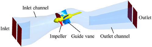
FIGURE 1. Three-dimensional model of slanted axial-flow pump.

All the simulations were performed using the commercial software ANSYS Fluent 18.0. ICEM was used to generate the unstructured grid (Chen et al., 2016; 2021) to match the axial-flow pump. The schematic diagram of the grid is presented in Figure 2.

FIGURE 2

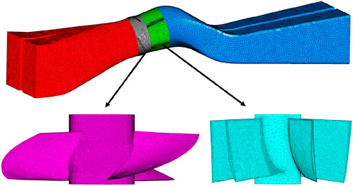
FIGURE 2. Grid diagram of the computational domain.

To ensure the reliability of the numerical simulation, six sets of grids from coarse to fine were selected and relevant data are shown in Figure 3. Once the number of the grid elements reached a certain order of magnitude (i.e., N > 2 million), there would be no significant influence on the numerical simulation result of the efficiency. The number of grid points used in the simulation was 2.9 million. The numbers of grid elements of the inlet channel, outlet channel, guide vane section, and impeller section were determined to be 0.68, 0.75, 0.7, and 0.8 million, respectively.

FIGURE 3

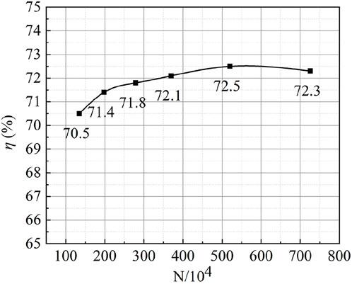
FIGURE 3. Efficiency of axial-flow pump system with different numbers of grid elements.

2.3 Computational set-up

A mass flow inlet was applied to the inlet of the domain, and the outlet boundary condition was set to zero pressure. No-slip boundary conditions were applied at the channel walls. A standard wall function was selected to model the turbulent boundary layers. The interface was used to transfer information between each computing area. To guarantee reliability and accuracy, the convergence residual was set to 10⁻⁵ (Kan et al., 2022).

2.4 Equivalent sand grain model

The roughness constant Cs and equivalent sand height Ks can be achieved in Fluent. The roughness constant Cs had little effect on the hydraulic performance of the pump with a high specific speed. The specific speed of the axial-flow pump in this work was very high, with a value of 1,450. Therefore, we neglected the roughness constant Cs in the numerical simulations and focused on the influence of the equivalent sand height Ks on the hydraulic performance of the axial-flow pump device. In engineering, the roughness Ra describes the surface roughness of the material during processing. The equivalent sand particle height Ks is based on an arranged row of uniform small balls. The formula relating the equivalent sand height Ks and the surface roughness Ra is as follows (Feng et al., 2016):

$Ks=11.0293Ra(6)$

The effect of roughness on the flow pattern inside the pump unit was incorporated via a wall function, where a term ∆B was added. Different roughness values would produce different ∆B values, which would affect the flow near the wall. The wall function considering the wall roughness is shown as follows:

$u^{+}=\frac{1}{\kappa }In\left(E{y}^{+}\right)-\mathrm{\Delta }B(7)$

where u⁺ is the dimensionless velocity, κ and E are empirical constants, which were 0.4187 and 9.793, respectively, and y+ is the dimensionless wall normal distance.

3 Results and analysis

3.1 Model test and validation

To verify the reliability of the numerical simulation model, experiments were performed under the same operating conditions. As shown in Figure 4, the head and efficiency of the simulation results were in great agreement with those of the experiment. The maximum relative errors of the head and efficiency between the simulation and the experimental result were 4.4% and 4.1%, respectively. The error between them may have been related to the high experimental error, due to the smooth wall adopted in the simulation. Overall, the comparison proved that the numerical simulation method utilized in this work could accurately predict the external characteristics of the slanted axial-flow pump and the simulation results were reliable.

FIGURE 4

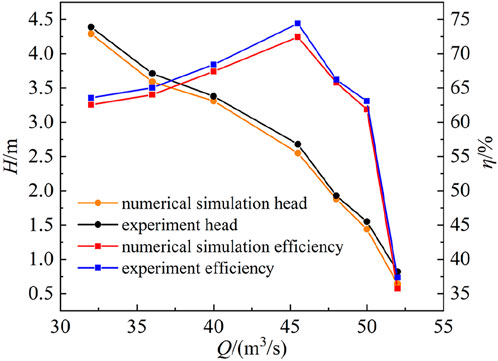
FIGURE 4. Comparison of the head and efficiency of the slanted axial-flow pump.

3.2 Hydraulic performance of flow components with different Ra values

In this work, we set three roughness Ra values for different flow components of the axial-flow pump (channel, guide vane, and impeller). Figure 5 shows the variation in the head and efficiency of the slanted axial-flow pump devices with different roughness values and flow rates. For example, for Ra = 100 μm (Figure 5B), compared with the pump device with smooth walls, when Q = 0.7Q₀, the efficiencies of the devices with different rough sections (channel, guide vane, and impeller) decreased by 0.86%, 1.44%, and 1.98%, respectively, and the corresponding heads decreased by 0.04, 0.05, and 0.08 m. Under the designed condition, the efficiencies of the device with different rough sections decreased by 0.52%, 0.89%, and 1.31%, and the corresponding heads decreased by 0.15, 0.17, and 0.2 m respectively. When the flow rate increased, the efficiencies and heads of the devices further decreased. Under different flow conditions, the addition of roughness to the wall of the impeller chamber caused the largest reduction of the efficiencies and heads, followed by the guide vane chamber, and the inlet and outlet channel had the least impact.

FIGURE 5

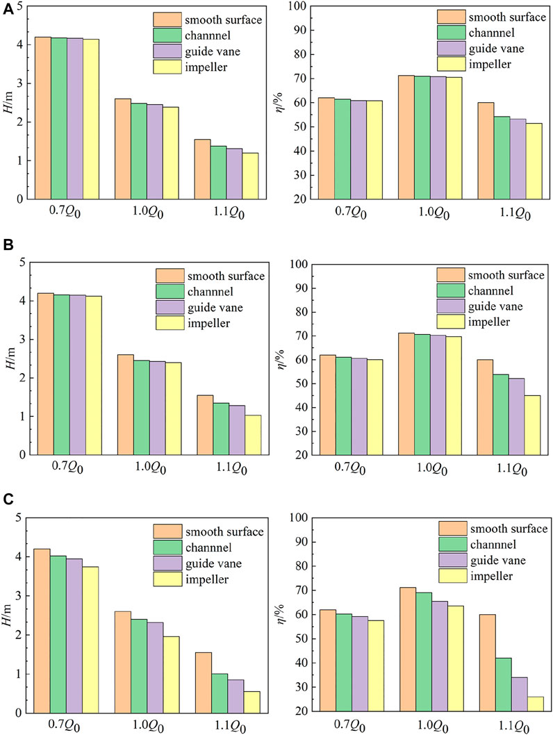
FIGURE 5. Variations in the heads and efficiencies of axial-flow pump devices: (A) Ra = 10 μm, (B) Ra = 100 μm, and (C) Ra = 1,000 μm.

The hydraulic losses of the slanted axial-flow pump devices with different roughness values of the flow components are plotted in Figure 6. Under the small-flow-rate condition (Q = 32 m³/s), the hydraulic losses of the pump devices with Ra = 100 μm at the inlet and outlet channel walls, guide vane chamber wall, and impeller chamber wall were 0.29, 0.42, and 0.71 m, respectively. Under the designed flow condition (Q = 45.5 m³/s), the hydraulic losses of the three pump devices with roughness values set for different flow components were 0.15, 0.3, and 0.62 m, respectively. Under the condition of a large flow rate (Q = 50 m³/s), the hydraulic losses of the three changed to 0.38, 0.62, and 1 m, respectively. Under the large-flow-rate condition, the hydraulic loss increased faster by adding roughness to the impeller chamber wall. The influence of the impeller chamber wall roughness on the hydraulic loss of the pump device was the largest.

FIGURE 6

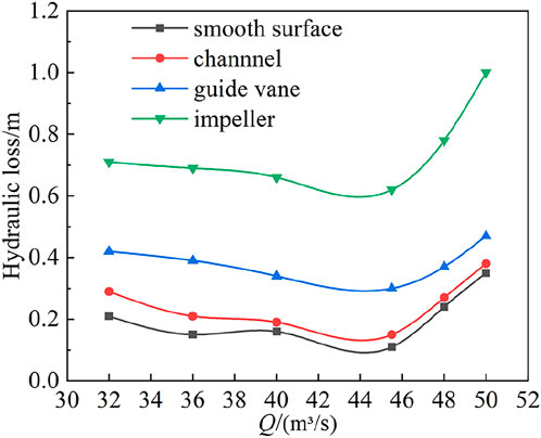
FIGURE 6. Hydraulic losses of different flow components with wall roughness.

For the convenience of discussion, the slanted axial-flow pump device with inlet and outlet flow channel roughness is named the CR pump, the slanted axial-flow pump device with guide vane chamber roughness is named the GVR pump, and the slanted axial-flow pump with impeller chamber roughness is named the IR pump. Figure 7 shows the 3D streamlines in the outlet channel of the axial-flow pump devices with different roughness values of the flow components. The roughness was specified as Ra = 100 μm. Under the condition of a small flow rate, the streamlines of the GVR, and CR pump devices were relatively smooth, and the flow was deflected from the left side. Partial reflux occurred in the right flow channel of the IR pump. Under the specified flow rate, the streamlines of the IR pump were smooth, and the flow pattern was relatively good. Under the condition of a large flow rate, the streamlines in the outlet channel were disordered, and a significant reflux phenomenon occurred in the right outlet channel, which affected the performance of the IR pump device. Compared with the IR pump device, the flow patterns of the GVR, and CR pump devices were better. The 3D streamlines of the outlet channel showed that the wall roughness had a greater impact on the flow pattern of the IR pump than those of the GVR and CR pumps.

FIGURE 7

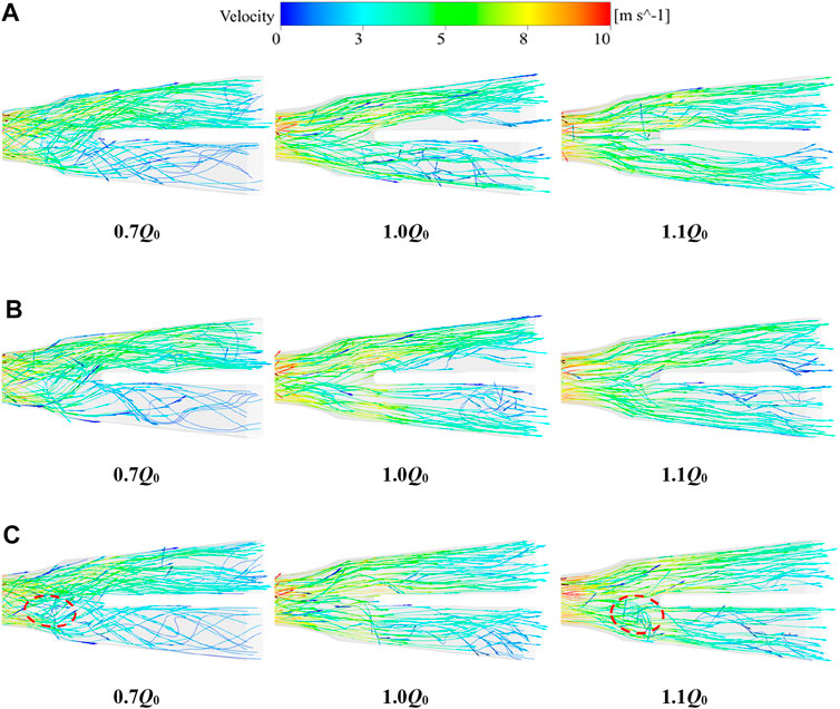
FIGURE 7. Three-dimensional Streamlines in the outlet channel: (A) IR pump, (B) GVR pump, and (C) CR pump.

Under the condition of a large flow rate, the hydraulic performances of the pumps were significantly different, so this condition was selected to analyze the difference after adding roughness to the flow components. Figure 8 shows the distributions of the pressure, vorticity, and turbulent kinetic energy (TKE) near the tip region (R* = 0.95). There were no significant differences in the pressure and vorticity, and the differences between the pump devices with rough flow components were reflected in the TKE distribution. The TKE of the IR pump naturally increased significantly due to the roughness being set directly in the runner chamber. In addition, the pressure on the suction surface of the IR pump increased, and the negative pressure decreased. The vorticity also increased compared to those of the other two pump devices. The TKE of the CR pump was larger than that of the GVR pump at the runner inlet because the TKE increased after the roughness of the inlet flow channel was set. The GVR pump only had increased roughness in the guide vane chamber, which hardly affected the TKE of the runner inlet.

FIGURE 8

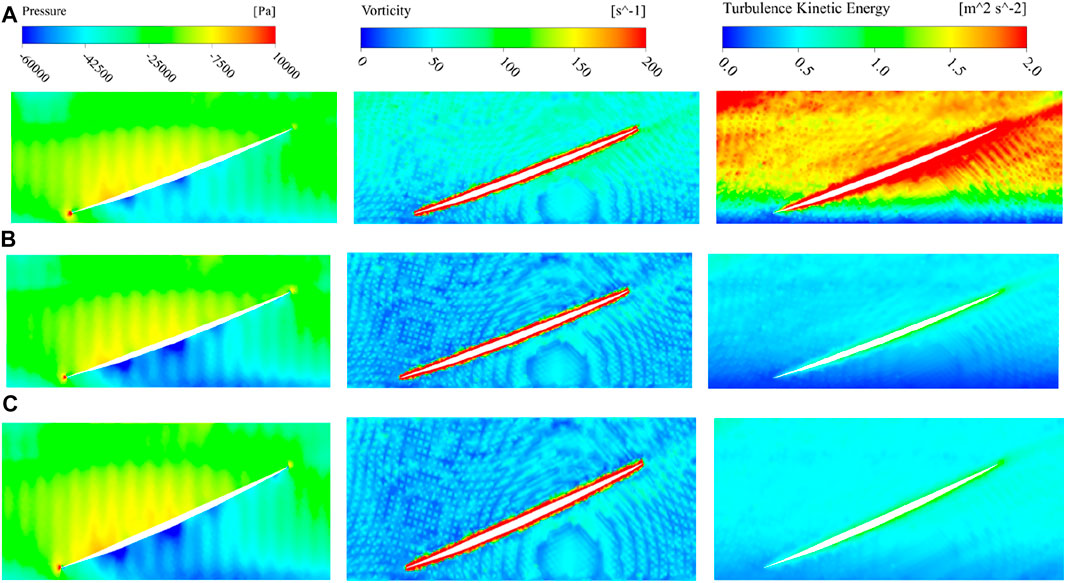
FIGURE 8. Distributions of pressure, vorticity, and turbulent kinetic energy (TKE) near the tip region (R* = 0.95): (A) IR pump, (B) GVR pump, and (C) CR pump.

3.3 Analysis of IR pump performance with different Ra values

Figure 9 shows the external characteristic curves of IR pumps with different Ra values. From Figure 9A, it can be seen that the smaller the roughness the IR pumps had, the closer the head values were to those calculated by the smooth wall condition. At the same time, the head curves showed a gradual downward trend with the increase in the flow rate. Under the same flow rate condition, the head gradually decreased with the increase in the roughness. It is worth noting that under the condition with a large flow rate (Q = 52 m³/s) when the roughness of the IR pump increased from 0 to 960 μm, the pump device changed from pump conditions to turbine conditions. When Ra was in the range of (0 μm, 60 μm), the increase in the roughness had little effect on the head of the device. When Ra was in the range of (60 μm, 960 μm), the effect of the roughness on the head of the device was significant. This indicated that the head of an inclined axial-flow pump device is greatly affected by roughness when it is running under the large-flow-rate condition.

FIGURE 9

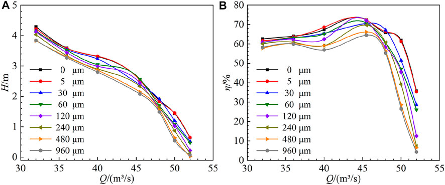
FIGURE 9. Head and efficiency of IR pumps with different roughness values: (A) H versus Q and (B) η versus Q.

From Figure 9B, it can be seen that the efficiencies of the IR pumps with smaller roughness values were closer to those with smooth wall conditions. With the increase in the flow rate, the efficiency of the device increased gently first and then decreased rapidly after the optimal operating point. The flow rate of the optimal operating point was Q = 45.5 m³/s. When the flow rate was fixed, the device efficiency decreased significantly with the increase in the roughness. With the increase in the roughness, the friction loss caused by the fluid flowing through the wall boundary layer increased, which was significant under the condition with a large flow rate. When the roughness increased from 0 to 960 μm, the pump device changed from pump conditions to turbine conditions. Under the condition of a small flow rate, the influence of the wall roughness on the device efficiency was relatively small, followed by the designed flow rate condition, and the largest influence was under the large-flow-rate condition.

Figure 10 shows the impeller torques of the IR pumps with different Ra values. Under the condition of a small flow rate, the impeller torques were 1,68,054.09, 1,67,631.29, 1,67,379.05, 1,66,039.27, 1,65,088.09, 1,62,854.3, and 1,62,253.33 Nm for Ra = 5, 30, 60, 120, 240, 480, and 960 μm. Compared to the pump with a smooth wall, the impeller torques of the IR pumps decreased by 0.31%, 0.56%, 0.71%, 1.5%, 2.7%, 3.4%, and 3.8%, respectively. Under the designed flow condition, when Ra = 5, 30, 60, 120, 240, 480, and 960 μm, the impeller torque was 1,22,183, 1,18,244, 1,21,493, 1,18,553, 1,16,786, 1,13,763, and 1,12,622 Nm, respectively. Compared with the pump with smooth walls, impeller torques of the IR pumps decreased by 0.19%, 3.4%, 0.75%, 3.16%, 4.6%, 7.6%, and 8%, respectively. The impeller torques were 73,989, 72,688, 71,367, 70,293, 68,682, 64,728, and 63,232 N when Ra = 5, 30, 60, 120, 240, 480, and 960 μm at a large flow rate.

FIGURE 10

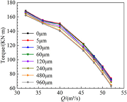
FIGURE 10. Impeller torque of IR pumps with different Ra values.

The outlet flow field of the guide vane can be evaluated by the axial velocity distribution uniformity coefficient ω and velocity-weighted average drift angle of water flow θ. The closer ω is to 100%, a smaller θ represents a better flow pattern of the outlet flow field, and the hydraulic loss is relatively small. The formulas for ω and θ are as follows (Zhu et al., 2007; Yang et al., 2012):

$\omega =\left[1-\frac{1}{V_{\text{a}}}\sqrt{{\displaystyle \sum _{i=1}^n\left[\left(V_{\mathrm{ai}}-V_a\right)\right]}}\right]\times 100\text{\%}(8)$

$\theta ={\displaystyle \sum _{i=1}^n{V}_{\text{ai}}\left\{90°{-\text{tg}}^{-1}\frac{V_{\mathit{ti}}}{V_{\mathit{ai}}}\right\}/{\displaystyle \sum _{i=1}^n{V}_{\mathit{ai}}}}(9)$

where V_a is the arithmetic mean value of the axial velocity at the section of the guide vane outlet, V_ai is the axial velocity of each calculation unit of the section, V_ti is the transverse velocity of each calculation unit of the section, and n is the number of calculation units on the section. In this work, n was equal to 200.

Figure 11 shows the influence of the roughness on ω and θ under different flow rate conditions. From Figure 11A, we see that the axial velocity distribution uniformity coefficient ω was the highest at the optimal condition point. With the increase in the roughness from 0 to 960 μm, the axial velocity uniformity decreased from 81.2% to 75.5%. Under the small-flow-rate condition, the axial distribution uniformity coefficient curve trend was similar to that of the designed flow condition, and the overall downward migration was about 3 percentage points. Under the condition of a high flow rate, the uniformity of the axial velocity distribution was the lowest. As the roughness increased from 0 to 960 μm, the uniformity of axial velocity distribution decreased from 72% to 56.5%. Under the pump conditions, the increase in the wall roughness led to a decrease in the axial velocity distribution uniformity, especially when the flow rate was large. From Figure 11B, it can be seen that at the optimal condition point, the velocity weighted average flow angle was the smallest. With the increase in the roughness from 0 to 960 μm, the velocity-weighted average drift angle increased from 6.85° to 10.55°. Under the condition of a small flow rate (Q = 0.7Q₀), the velocity-weighted average drift angle curve was similar to that under the designed condition, with an overall increase of 1°–2°. Under the condition of a large flow rate (Q = 1.1Q₀), the velocity-weighted average drift angle was the largest. With the increase in the roughness from 0 to 960 μm, the velocity-weighted average drift angle increased from 8.21° to 12.55°. We can infer that the increase in the wall roughness leads to increases in the velocity weighted average deviation angle and the axial velocity distribution uniformity coefficient, and the increases are more significant under the large-flow-rate condition.

FIGURE 11

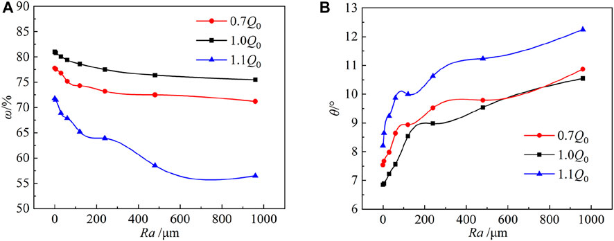
FIGURE 11. Effect of roughness on ω and θ under different flow rate conditions: (A) ω versus Ra and (B) θ versus Ra.

Figure 12 shows the effect of roughness on the hydraulic losses of the IR pumps under different flow rate conditions. With the increase in the roughness, the hydraulic loss increased. The hydraulic loss of the IR pump with Ra = 5 μm was close to that with smooth walls. With the increase in the roughness, the hydraulic loss increased. When Ra = 960 μm, the hydraulic loss was the largest under all flow rate conditions relative to that of the smooth wall condition. Under the condition with a small flow rate, the hydraulic loss was 0.58 m. Under the designed flow conditions, the hydraulic loss was 0.42 m. Under the condition with a large flow rate, the hydraulic loss was 0.78 m. Regardless of what the roughness was, the loss of the designed flow condition was the smallest compared with the other groups. When the flow rate was large, the increase in hydraulic loss was slower in the Ra range of (5 μm, 60 μm) and faster in the Ra range of (60 μm, 960 μm).

FIGURE 12

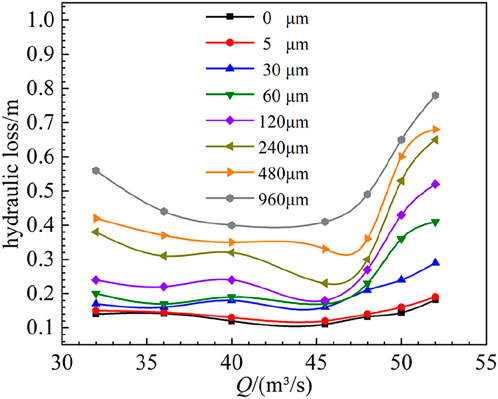
FIGURE 12. Effect of roughness on the hydraulic loss.

To study the effect of wall roughness on the internal flow field, a total of 21 monitoring points were arranged on the surface of the blade, as shown in Figure 13. A0–A7 were arranged on span 0.9 near the outer edge of the blade, P0–P7 were arranged on span 0.5 along the flow direction center of the impeller, and B0–B4 were arranged on span 0.1 near the root of the blade.

FIGURE 13

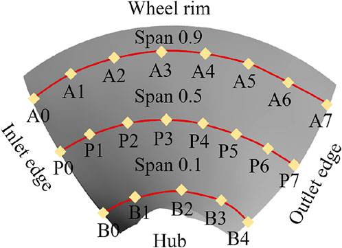
FIGURE 13. Monitoring point layout in blade working face.

Figure 14 shows the static pressure distributions of the blade pressure surface under three different flow rate conditions. The static pressure value of the blade surface layer was large, and the static pressure value of the blade root near the hub was small. Under the condition of a small flow rate, the static pressure value increased gradually along the flow direction, and the pressure value near the outlet of the blade near the rim reached the highest value. Under the designed flow condition and the large-flow-rate condition, the radial static pressure value increased hierarchically along the pressure surface. There was a negative pressure near the hub because the fluid flowed through the runner blade from the inlet channel, and only a small part of the separated fluid passed through the impeller near the hub. The energy obtained by the impeller near the hub was lower, so there was a local negative pressure on the surface of the blade near the hub, which greatly increased the possibility of cavitation.

FIGURE 14

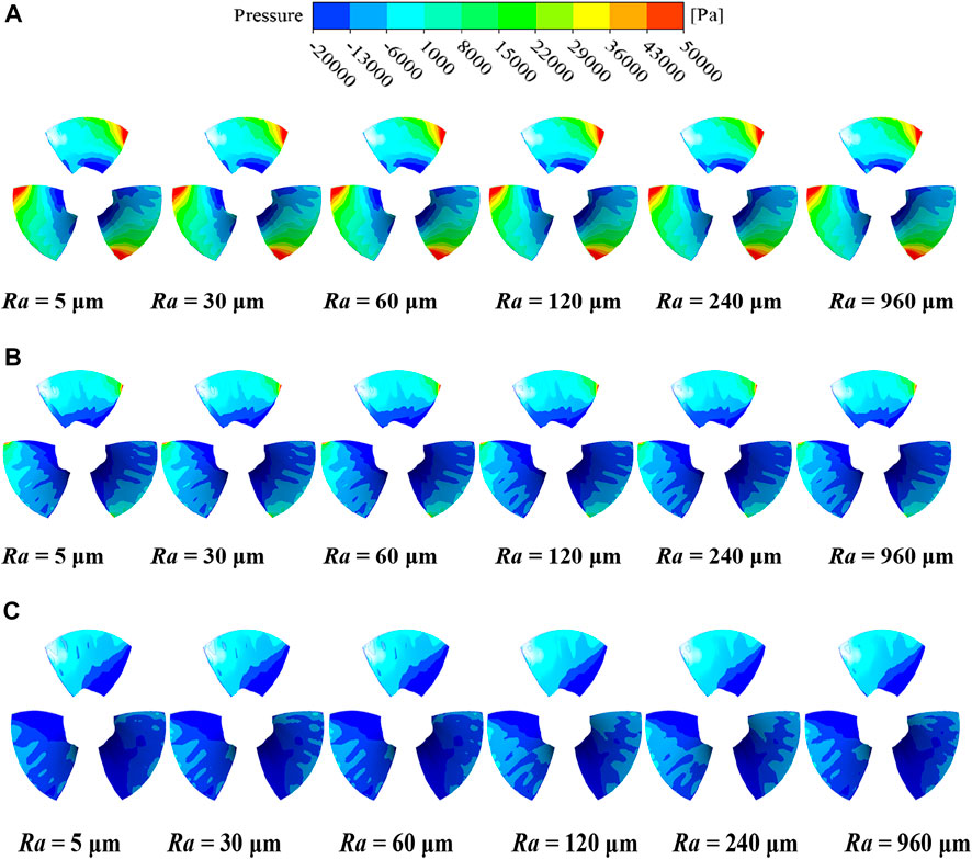
FIGURE 14. Static pressure distribution of blade working face: (A) 0.7Q₀, (B) 1.0Q₀, and (C) 1.1Q₀.

Under the same flow rate condition, with the increase in the roughness, the range of the negative pressure zone increased significantly. When the IR pumps had the same roughness, with the increase in the flow rate, the static pressure value of the pressure surface decreased. Under the condition of a small flow rate, the static pressure value of the pressure surface was larger than that of the designed flow rate and the large flow rate. This was because, under the condition of a small flow rate, the flow velocity near the pressure surface of the blade was larger, and the flow pattern disorder near the blade caused an increase in energy loss. The increase in the roughness may account for the cavitation. Near the pressure surface of the impeller outlet, under the same pressure level, the range of the high-pressure zone was the largest under the condition of a small flow rate, followed by the designed flow rate high, while the pressure zone was not evident under the large-flow-rate condition. This also verified that the H versus Q curve (Figure 9A) decreased with the increase in the flow rate.

Figure 15 shows the variations in the histogram of the monitoring points on the blade working surface with the roughness in the designed flow rate condition. With the increase in the wall roughness, the energy loss near the boundary layer increased, resulting in a decrease in the static pressure value at the monitoring point. Figure 15A indicates that the static pressure values at span 0.1 near the blade root were generally smaller than those at span 0.5 and span 0.9. When Ra = 960 μm, the static pressure values of points B0–B4 ranged from 33,544 to 46,254 Pa. Compared with their static pressure values at Ra = 5 μm, they decreased by 20.8%, 19%, 20.16%, and 13%. Figure 15B shows that the static pressure value of the monitoring point P0 in the smooth wall condition was 75,887 Pa, and the static pressure value of the impeller pressure surface under the wall with different Ra values was lower than that under the smooth wall condition. Thus, at the P0 monitoring point, when the roughness was greater than 240 μm, the roughness had a significant influence on the wall static pressure value. The variation trend of the static pressure value of the pressure surface at monitoring points P2 and P5 with the roughness was similar to that at P0. At monitoring point P7, the static pressure value of the pressure surface in the smooth wall condition was 1,81,423 Pa. With the increase in the roughness, the static pressure value of the pressure surface under each roughness condition decreased by 0.08%, 0.12%, 3.5%, 7%, 13.4%, 20.2%, and 30.1%, respectively. We infer that when the roughness was less than 30 μm, the roughness had little effect on the static pressure value of monitoring point P7, which was set at the impeller outlet. It can be seen from Figure 15C that the static pressure value of span 0.9 near the blade’s outer edge was larger than that of span 0.5 overall, and the static pressure value decreased with the increase in the roughness. When Ra = 960 μm, the static pressure values of A0, A2, A5, and A7 were 69,875, 81,544, 1,25,424, and 1,52,125 Pa, respectively. Compared with those at Ra = 5 μm, the static pressure values decreased by 15.3%, 27.4%, 18.8%, and 25.6%, respectively. When Ra was in the range of (5 μm, 120 μm), the decrease in the static pressure of the blade was larger. When Ra was in the range of (120 μm, 960 μm), the decrease in the static pressure of the blade was smaller.

FIGURE 15

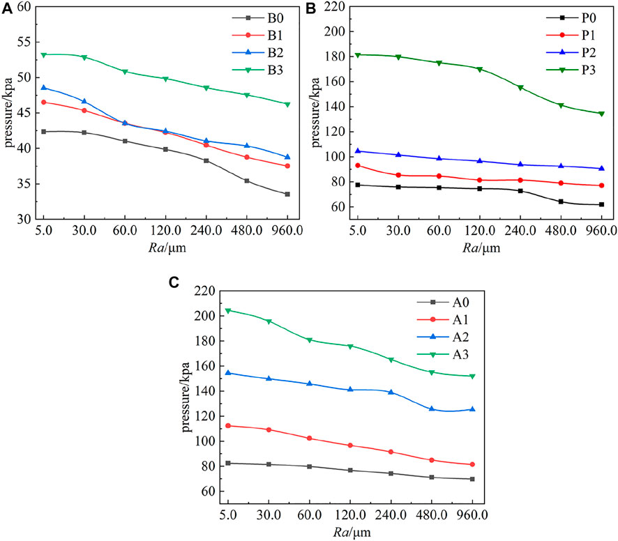
FIGURE 15. Static pressure variations with roughness at different monitoring point: (A) span 0.1, (B) span 0.5, and (C) span 0.9.

The influence of the roughness on the TKE of the blade pressure surface and the suction surface under the three flow rate conditions is shown in Figure 16. The turbulent kinetic energy increased with the increase in the roughness, which indicated that the energy loss near the boundary layer increased, and it is also an important reason for the decrease in the pump efficiency. Figure 16A shows that with different Ra values, the turbulent kinetic energy of the pressure surface was about 0.46 m²/s². The turbulent kinetic energy on the pressure surface was about 48% smaller than that under the designed flow condition, and it was about 52.8% smaller than that under the large-flow-rate condition. With the same roughness, the turbulent kinetic energy of the pressure surface was the largest under the large-flow-rate condition, followed by the designed flow condition, and the turbulent kinetic energy of the pressure surface was the smallest under the small-flow-rate condition.

FIGURE 16

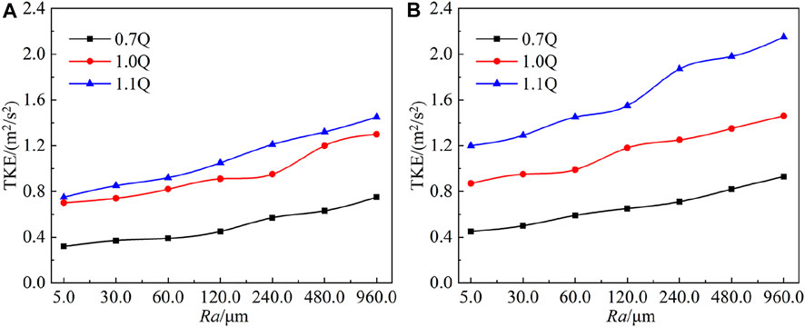
FIGURE 16. Variations of turbulent kinetic energy with different Ra values: (A) pressure surface and (B) suction surface.

It can be seen from Figure 16B that when Ra was in the range of (5 μm, 60 μm), the corresponding turbulent kinetic energy ranged from 0.45 to 0.59 m²/s², with values that were 48.2%, 47.3%, and 40.4% smaller than that under the designed flow condition, and 2.5%, 61.2%, and 59.3% smaller than that under the large-flow-rate condition. When Ra was in the range of (120 μm, 960 μm), the turbulent kinetic energy ranged from 0.65 to 0.93 m²/s² at a small flow rate, which was about 40.9% lower than that of the designed flow rate and about 58.8% lower than that at the large flow rate. Under different flow rate conditions, with the increase in the roughness, the turbulent kinetic energy of the pressure surface increased gradually.

The comparison of the turbulent kinetic energy of the pressure surface in Figure 16A and the suction surface in Figure 16B showed that when the flow rate was small, the turbulent kinetic energy of the blade suction surface was generally greater than that of the blade pressure surface. Due to the small-flow-rate condition, the impeller inlet water had adverse flow patterns, such as vortices and backflow, which caused high turbulent kinetic energy to be created at the blade suction surface. Under the designed flow condition, when the wall roughness values were 5, 30, 60, 120, 240, 480, and 960 μm, the corresponding turbulent kinetic energies on the pressure surface were 0.7, 0.74, 0.82, 0.91, 0.95, 1.2, and 1.3 m²/s², respectively. The turbulent kinetic energy of the suction surface ranged from 0.87 to 1.46 m²/s². The turbulent kinetic energy of the suction surface was higher than that of the pressure surface by 24.2%, 28.4%, 15.9%, 29.7%, 31.5%, 11.1%, and 12.3% respectively. When the flow rate increased to 1.1Q, the corresponding turbulent kinetic energies on the pressure surface were 0.75, 0.85, 0.92, 1.05, 1.21, 1.32, and 1.45 m²/s², respectively.

4 Conclusion

In this study, simulations were performed, and the performance of the slanted axial-flow pump under the effects of wall roughness and flow rates was analyzed. The specific conclusions are as follows:

1) Model tests of slanted axial-flow pump devices were carried out, and the consistency between the model test results and the numerical simulation results showed that the numerical method used in this article was credible.

2) The influence of the roughness of the different flow components on the hydraulic performance of the pump devices under different flow rate conditions was studied. From the perspective of external characteristics, the device efficiency and head of the IR pump devices were the lowest, and the hydraulic loss was the highest. From the perspective of the internal flow characteristics, the roughness of the impeller chamber wall had a slight influence on the flow pattern of the device, and backflow and vortices appeared in the device under the large-flow-rate condition. The roughness of the impeller chamber wall had the greatest impact on the hydraulic performance of the pump device, followed by the roughness of the guide vane chamber, and the roughness of the inlet and outlet flow channel had the smallest impact.

3) The influence of different roughness values on the hydraulic performance of the IR pump device was studied. The optimal working condition of the pump was obtained, which was a flow rate of 45.5 m³/s. The flow-head curve of the pump device showed a downward trend with the increase in the flow rate. The flow efficiency characteristic curve showed a trend of first increasing and then decreasing. Under the condition of a large flow rate, the curve dropped faster. Under the same flow rate condition, the increase in the roughness caused a decrease in the head, efficiency, torque, and surface static pressure of the blade pressure surface. When Ra was in the range of (0 μm, 60 μm), the roughness had little effect on the performance parameters. While a roughness Ra beyond 60 μm had a significant effect on the performance parameters. With the increase in the roughness, the hydraulic loss and turbulent kinetic energy of the device increased since the energy loss on the boundary layer in the device increased, which was more significant under the large-flow-rate condition. With the increase in the roughness, the uniformity of the axial-flow velocity distribution coefficient decreased, and the velocity-weighted average bias angle increased, which was responsible for the decrease in the device performance.

Data availability statement

The raw data supporting the conclusion of this article will be made available by the authors, without undue reservation.

Author contributions

Conceptualization: YC and HC; methodology: ZL, YG, and JZ; software: QS, ZL, and JZ; validation: YC and HC; formal analysis: YC, QS, ZL, and HC; resources: YC and HC; writing and original draft preparation, YC, QS, ZL, YG, and JZ; writing-review and editing: YC and HC; funding acquisition: HC.

Funding

This research was funded by the National Natural Science Foundation of China (52006053), Natural Science Foundation of Jiangsu Province (BK20200508), China Postdoctoral Science Foundation (2021M690876), and Postdoctoral Research Fund of Jiangsu Province (2021K498C). The computational work was supported by the High Performance Computing Platform, Hohai University. The support of Hohai University, China, is also gratefully acknowledged.

Conflict of interest

The authors declare that the research was conducted in the absence of any commercial or financial relationships that could be construed as a potential conflict of interest.

Publisher’s note

All claims expressed in this article are solely those of the authors and do not necessarily represent those of their affiliated organizations, or those of the publisher, the editors, and the reviewers. Any product that may be evaluated in this article, or claim that may be made by its manufacturer, is not guaranteed or endorsed by the publisher.

References

Chen, E. Y., Ma, Z. L., Zhao, G. P., Li, G. P., Yang, A. L., Nan, G. F., et al. (2016). Numerical investigation on vibration and noise induced by unsteady flow in an axial-flow pump. J. Mech. Sci. Technol. 30 (12), 5397–5404. doi:10.1007/s12206-016-1107-4

CrossRef Full Text | Google Scholar

Chen, H., Zhou, D., Kan, K., Guo, J., Zheng, Y., Binama, M., et al. (2021). Transient characteristics during the co-closing guide vanes and runner blades of a bulb turbine in load rejection process. Renew. Energy 165, 28–41. doi:10.1016/j.renene.2020.11.064

CrossRef Full Text | Google Scholar

Deng, L., Yong, K., Wang, X., Ding, X., and Fang, Z. (2016). Effects of nozzle inner surface roughness on the cavitation erosion characteristics of high speed submerged jets. Exp. Therm. Fluid Sci. 74, 444–452. doi:10.1016/j.expthermflusci.2016.01.009

CrossRef Full Text | Google Scholar

Echouchene, F., Belmabrouk, H., Penven, L. L., and Buffat, M. (2011). Numerical simulation of wall roughness effects in cavitating flow. Int. J. Heat Fluid Flow 32 (5), 1068–1075. doi:10.1016/j.ijheatfluidflow.2011.05.010

CrossRef Full Text | Google Scholar

Fei, Z., Xu, H., Zhang, R., Zheng, Y., Mu, T., Chen, Y., et al. (2022a). Numerical simulation on hydraulic performance and tip leakage vortex of a slanted axial-flow pump with different blade angles. Proc. Institution Mech. Eng. Part C J. Mech. Eng. Sci. 236 (6), 2775–2790. doi:10.1177/09544062211032989

CrossRef Full Text | Google Scholar

Fei, Z., Zhang, R., Xu, H., Feng, J., Mu, T., Chen, Y., et al. (2022b). Energy performance and flow characteristics of a slanted axial-flow pump under cavitation conditions. Phys. Fluids 34 (3), 035121. doi:10.1063/5.0085388

CrossRef Full Text | Google Scholar

Feng, J., Zhu, G., He, R., Luo, X., and Lu, J. (2016). Influence of wall roughness on performance of axial-flow pumps. J. Northwest A F Univ. Nat. Sci. Ed. 44 (3), 196–202. doi:10.13207/j.cnki.jnwafu.2016.03.027

CrossRef Full Text | Google Scholar

Hu, W., Tong, D., Li, Z., Wang, R., and Yang, F. (2021). Numerical analysis of internal flow in a slanted axial-flow pump. J. Irrigation Drainage 40 (11), 66–72. doi:10.13522/j.cnki.ggps.2021247

CrossRef Full Text | Google Scholar

Kan, K., Chen, H., Zheng, Y., Zhou, D., Binama, M., Dai, J., et al. (2021a). Transient characteristics during power-off process in a shaft extension tubular pump by using a suitable numerical model. Renew. Energy 164, 109–121. doi:10.1016/j.renene.2020.09.001

CrossRef Full Text | Google Scholar

Kan, K., Zhang, Q., Xu, Z., Chen, H., Zheng, Y., Zhou, D., et al. (2021b). Study on a horizontal axial-flow pump during runaway process with bidirectional operating conditions. Sci. Rep. 11 (1), 21834. doi:10.1038/s41598-021-01250-1

PubMed Abstract | CrossRef Full Text | Google Scholar

Kan, K., Zhang, Q., Xu, Z., Zheng, Y., Gao, Q., Shen, L., et al. (2022). Energy loss mechanism due to tip leakage flow of axial flow pump as turbine under various operating conditions. Energy 255, 124532. doi:10.1016/j.energy.2022.124532

CrossRef Full Text | Google Scholar

Kang, Y. S., Yoo, J. C., and Kang, S. H. (2006). Numerical predictions of roughness effects on the performance degradation of an axial-turbine stage. J. Mech. Sci. Technol. 20 (7), 1077–1088. doi:10.1007/bf02916007

CrossRef Full Text | Google Scholar

Long, L., and Wang, Z. (2004). Simulation of the influence of wall roughness on the performance of axial-flow pumps. Trans. Chin. Soc. Agric. Eng. 1, 132–135. doi:10.1300/J064v24n01_09

CrossRef Full Text | Google Scholar

Marzabadi, F. R., and Soltani, M. R. (2013). Effect of leading-edge roughness on boundary layer transition of an oscillating airfoil. Sci. Iran. 20 (3), 508–515. doi:10.1016/j.scient.2012.12.035

CrossRef Full Text | Google Scholar

Pang, A., Skote, M., and Lim, S. Y. (2016). Modelling high Re flow around a 2D cylindrical bluff body using the k-ω (SST) turbulence model. Prog. Comput. Fluid Dyn. Int. J. 16 (1), 48. doi:10.1504/pcfd.2016.074225

CrossRef Full Text | Google Scholar

Qin, D., Huang, Q., Pan, G., Han, P., Luo, Y., Dong, X., et al. (2021). Numerical simulation of vortex instabilities in the wake of a preswirl pumpjet propulsor. Phys. Fluids 33 (5), 055119. doi:10.1063/5.0039935

CrossRef Full Text | Google Scholar

Ren, N. X., and Ou, J. P. (2009). Dust effect on the performance of wind turbine airfoils. J. Electromagn. Analysis Appl. 1 (2), 102–107. doi:10.4236/jemaa.2009.12016

CrossRef Full Text | Google Scholar

Shi, L., Zhang, W., Jiao, H., Tang, F., Wang, L., Sun, D., et al. (2020). Numerical simulation and experimental study on the comparison of the hydraulic characteristics of an axial-flow pump and a full tubular pump. Renew. Energy 153, 1455–1464. doi:10.1016/j.renene.2020.02.082

CrossRef Full Text | Google Scholar

Soltani, M. R., and Birjandi, A. H. (2013). Effect of surface contamination on the performance of a section of a wind turbine blade. Paper presented at the Aiaa Aerospace Sciences Meeting & Exhibit.

Google Scholar

Tao, B., Liu, J., Zhang, W., and Zou, Z. (2014). Effect of surface roughness on the aerodynamic performance of turbine blade cascade. Propuls. Power Res. 3 (2), 82–89. doi:10.1016/j.jppr.2014.05.001

CrossRef Full Text | Google Scholar

Walker, J., Flack, K., Lust, E., Schultz, M., and Luznik, L. (2013). The effects of blade roughness and fouling on marine current turbine performance. Paper presented at the European Wave & Tidal Energy Conference.

Google Scholar

Walker, J. M., Flack, K. A., Lust, E. E., Schultz, M. P., and Luznik, L. (2014). Experimental and numerical studies of blade roughness and fouling on marine current turbine performance. Renew. Energy 66, 257–267. doi:10.1016/j.renene.2013.12.012

CrossRef Full Text | Google Scholar

Wang, Z. W., Peng, G. J., Zhou, L. J., and Hu, D. Y. (2010). Hydraulic performance of a large slanted axial-flow pump. Eng. Comput. Swans. 27 (1-2), 243–256. doi:10.1108/02644401011022391

CrossRef Full Text | Google Scholar

Wang, C., Wang, F., Tang, Y., Zi, D., Xie, L., He, C., et al. (2020). Investigation into the phenomenon of flow deviation in the S-shaped discharge passage of a slanted axial-flow pumping system. J. Fluids Eng. 142 (4). doi:10.1115/1.4045438

CrossRef Full Text | Google Scholar

Wang, W., Tai, G., Pei, J., Pavesi, G., and Yuan, S. (2022). Numerical investigation of the effect of the closure law of wicket gates on the transient characteristics of pump-turbine in pump mode. Renew. Energy 194, 719–733. doi:10.1016/j.renene.2022.05.129

CrossRef Full Text | Google Scholar

Yang, F., Tang, F., and Liu, C. (2012). Numerical analysis on hydrodynamics of large-scale mixed-flow pump system. J. Hydroelectr. Eng. 31 (3), 217–222.

CrossRef Full Text | Google Scholar

Zhu, H. G., Yan, B. P., and Zhou, J. R. (2006). Study on the influence of wall roughness on the hydraulic performance of axial-flow pumps. J. Irrigation Drainage 1, 81–88. doi:10.13522/j.cnki.ggps.2006.01.020

CrossRef Full Text | Google Scholar

Zhu, H., Yuan, S., Liu, H., and Shi, W. (2007). Numerical simulation of the 3-D flow of a volute-type discharge passage in large pumping stations. Trans. Chin. Soc. Agric. Mach. 10, 49–53. doi:10.3969/j.issn.1000-1298.2007.10.012

CrossRef Full Text | Google Scholar