Configuration-dispatch dual-layer optimization of multi-microgrid–integrated energy systems considering energy storage and demand response

1 Introduction

In September 2020, China announced that it would increase its autonomous national contribution and adopt more robust policies and measures to strive for CO₂ emissions to peak by 2030 and work toward carbon neutrality by 2060 (Li et al., 2021c; Tan et al., 2021). The energy sector is gradually transforming into a clean and low-carbon structure under the traction of carbon peaking and carbon neutrality targets. The integrated energy system (IES) uses renewable energy to improve the efficiency and cleanliness of end-use energy consumption, essential to achieving clean energy substitution and low-carbon sustainable development of energy (Zhang and Xu, 2018; Wang et al., 2022). Its supply, distribution, and energy use links are highly coupled and have complex operational behavior. With the increase of integrated energy microgrids (MGs) in the same distribution area, the IES gradually evolves into a complex system incorporating cold, heat, and electrical multiple energy sources called the multi-microgrid (MMG)–integrated energy system (Li, 2021; Xiang et al., 2021). The complex coupling mechanism between multi-microgrids and multiple energy flows makes it difficult to apply traditional dispatching methods (Liu et al., 2020; Fan et al., 2022).

International researchers have extensively researched the optimal operation of multi-microgrid–integrated energy systems (Li et al., 2021b; Guo et al., 2021). Xu et al. (2018) established a day-ahead optimized economic dispatch model for multi-microgrid systems containing electrical energy interactions to minimize operating costs. In Gu et al. (2022), a cooperative operation model of MMG operators and load aggregators representing the benefits of entire MMG users is constructed based on Nash bargaining theory. It is demonstrated that the model can consider the economic benefits to society and individuals. In Wu et al. (2021a), an MMG electric energy sharing cooperative operation model is established for the MMG-integrated energy system based on the asymmetric Nash negotiation theory. A strategy is proposed to allocate the energy contribution based on the size of each MG to achieve a fair distribution of the cooperative benefits of each MG. Under the power market environment, an MMG energy trading mechanism based on the improved Nash bargaining method is designed to realize the microgrid group’s energy complementarity and maximize the microgrid group’s overall benefits (Shuai et al., 2021). Li et al. (2020) proposed a multi-objective optimal allocation method based on a negotiation game for MMGs with electrical energy interaction and an operation scheme to satisfy the economic benefits and efficient energy utilization of MMGs. The previous research has provided valuable ideas for dispatching the MMG-integrated energy system. However, the emphasis is on obtaining the economic benefits of system operation while neglecting new energy consumption and low-carbon operation.

With the promotion of the dual-carbon target, the pressure of new energy consumption further increases (Zhang et al., 2020b). As a flexible power source, energy storage can alleviate the intermittent nature of new energy, and a controlled load can alleviate the imbalance between power generation and consumption. The flexibility of resource access must be considered and fully utilized in the MMG-integrated energy system in the context of gradually increasing intermittent energy penetration. The notion of shared energy storage has progressively risen in recent years, enabling a new way of thinking to develop energy storage in MMGs. Wu et al. (2019) proposed a day-ahead optimal scheduling method for the combined cooling, heating, and power MMG system with a shared energy storage system (SESS), which reduces the system’s cost by coordinating the interactive electrical power between each MG and SESS. However, the study treats the shared energy storage side’s parameters as given values, and the results are too idealistic. In Wu et al. (2021a), a two-layer optimal configuration model of combined cooling, heating, and power MMG system considering the SESS is established to verify the economic advantages of SESS in the MMG system compared with self-built energy storage in each MG. Based on the improved Shapley method, Li et al. (2020) proposed an optimal allocation method for the SESS in the MMG system that uses energy storage to smooth out the net load fluctuations of MMGs and achieves fair cost-sharing among MGs to ensure the maximum benefit of each MG. Some scholars (Shuai et al., 2022) created a game model with economic benefits for MG operators, SESS operators, and user aggregators to achieve win–win outcomes for all three parties. In Gao and Ai (2021), a collaborative optimization method of internal and external full-time frame of the MMG system is introduced, which introduces a demand response mechanism in the MMG system, improves self-coordination and self-balancing ability among different resources, maximizes the use of renewable energy, and reduces the overall system cost. Li et al. (2019) suggested an MMG and multi-user Stackelberg game model with demand response, which allows for a balance between the MMGs’ tariff strategy and the users’ demand strategy and increases the overall economic benefits of MMGs. In a broader sense, the factors considered in the participation and dispatch of flexibility resources in the MMG-integrated energy system are relatively simple, focusing on achieving the balance of interests and shared governance decisions of multiple subjects through bargaining, cost-sharing, coordination, and optimization. However, the synergy of load and storage flexibility resources has not yet been fully exploited. The impact of renewable energy consumption and carbon emissions on the MMG-integrated energy system has not been considered.

As a result, this paper fully considers the influence of load and storage synergy on the dispatching operation of the MMG-integrated energy system and builds a dual-layer optimization model of MMG-integrated energy system configuration-dispatch considering energy storage and demand response to promote the consumption of new energy and reduce carbon emissions: 1) The upper layer optimizes the SESS for maximum annual profit, taking into account the charging and discharging constraints of energy storage as well as the power and capacity ceiling constraints, reasonably allocating the energy storage capacity in the MMG-integrated energy system, and transmitting the configuration results to the lower layer model. 2) The lower layer model improves the traditional carbon trading mechanism by including a dynamic incentive coefficient and proposing a technique for calculating carbon emissions from acquired power. 3) A low-carbon economic dispatch model for the MMG-integrated energy system is created using the improved carbon trading mechanism and load-side demand response, with the lowest annual operating cost as the optimization goal. 4) The effectiveness and rationale of the proposed dual-layer model are validated through a comparative analysis of several arithmetic test system scenarios.

The rest of this article is organized as follows: Section 2 introduces the MMG-integrated energy system framework. The demand response mechanism is introduced in Section 3. In Section 4, the configuration-scheduling dual-layer optimization model dispatch model is presented. Section 5 studies simulated cases to investigate the effectiveness of the proposed model. Finally, Section 6 concludes this article.

2 Framework of the MMG-integrated energy system

The MMG-integrated energy system integrates multiple energy sources such as electricity, heat, cooling, and gas, with external electricity supply from the upper distribution network and gas supply from the natural gas network. The interior comprises wind turbine (WT) and photovoltaic (PV) input devices, loads of multiple types of energy, and integrated energy use devices. The architecture of the MMG-integrated energy system is shown in Figure 1.

FIGURE 1

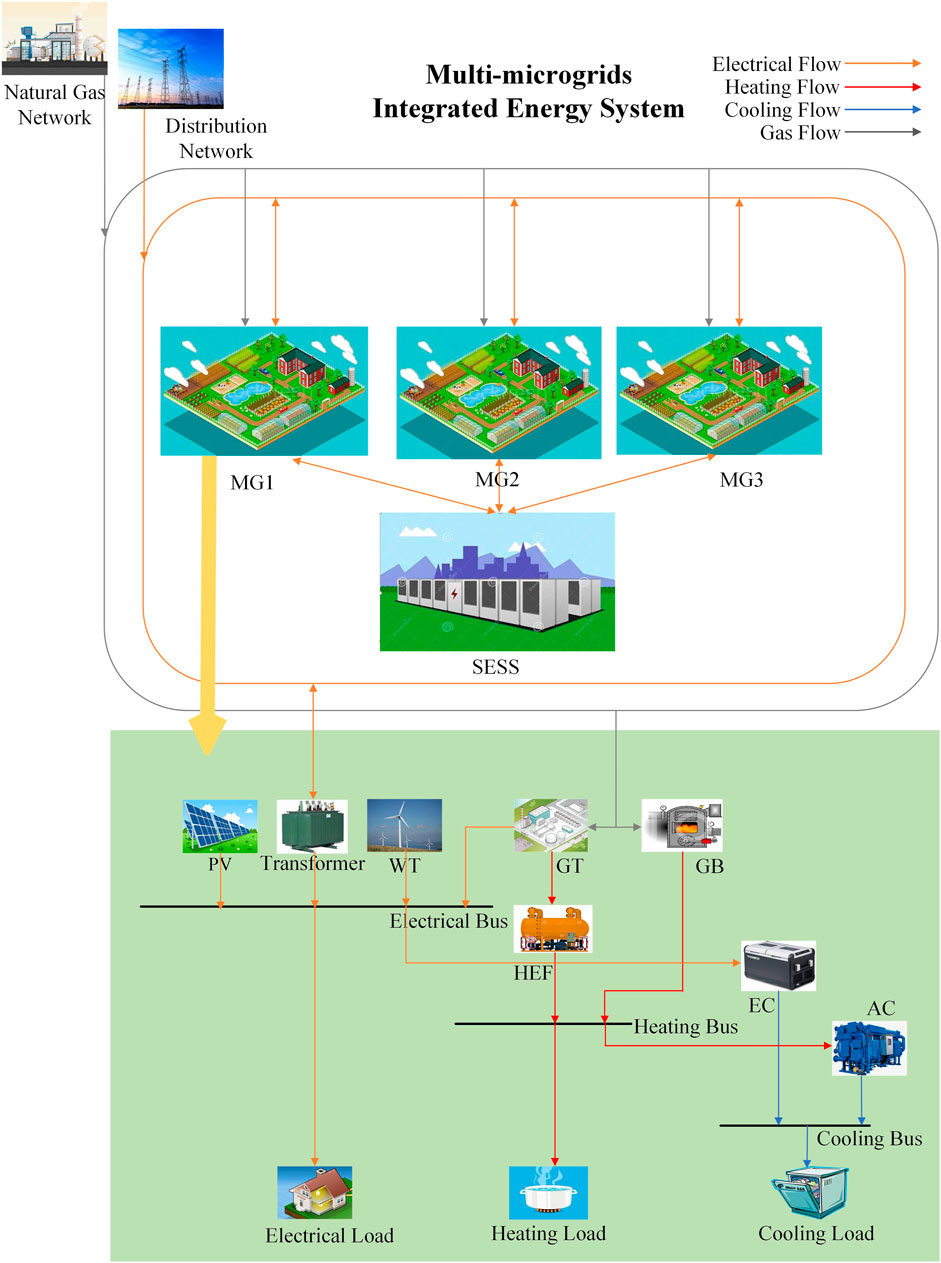
FIGURE 1. Architecture of the MMG-integrated energy system.

Developing energy storage equipment for individual MGs in an MMG-integrated energy system has high-cost and low-utilization issues. This paper introduces an SESS to interact with the MMGs for electric power and realizes the complete consumption of the power of WT and PV and the system’s economic and low-carbon operation by optimizing the capacity of shared energy storage and reasonably price planning the charging and discharging periods and power.

This paper focuses on the influence of SESS access on the economic and low-carbon efficiency of MMG-integrated energy systems rather than a complete examination of the SESS and benefit distribution between it and each microgrid. The operation mode of the SESS is briefly described as follows: The MMGs can freely interact with the SESS for electrical power, and if the MMGs have excess power, such as new energy power which is difficult to consume, they can sell the extra power to the SESS, generating revenue from electricity sales. If the MMGs need electricity, they can buy it from the SESS during peak hours or when there is low intermittent energy output. In addition to paying for the electricity purchased from shared energy storage, the multi-micro network also needs to pay service charges to the SESS in exchange for the shared energy storage service according to the amount of interacting electricity.

3 Demand response mechanism

The demand response (DR) of the load interacting within the MMGs replaces the one-way load management. The demand response modeling of electric, heating, and cooling loads in an MMG-integrated energy system is described below.

3.1 Electrical load demand response

This paper considers the price-type demand response of electrical load, and the load-side demand response behavior is refined for each comprehensive energy user. Users’ electricity demand and power consumption autonomy are guaranteed by guiding users to transfer electrical load according to time-of-use prices. The electrical load shifted by each customer during a specific dispatching period is counted and superimposed on the fixed electrical load to calculate the electrical load after demand response.

Take the MG a under Typical Day i as an example. The electrical load includes the fixed electrical load and transferable electric load. The fixed electrical load requires high reliability for system operation and is not transferable. The transferable electric load is relatively flexible and uses peak and valley time-sharing tariffs as a signal to guide users to transfer load from peak hours to valley hours. The electrical load demand response model can be expressed as follows:

$P_{\text{el,}i,a}\left(t\right)=P_{\text{fel,}i,a}\left(t\right)+P_{\text{tel,}i,a}\left(t\right)+P_{\text{tiel,}i,a}\left(t\right)(1)$

where P_el,i,a(t) denotes the electrical load in the period t and P_fel,i,a(t), P_tel,i,a(t), and P_tiel,i,a(t) denote the fixed electrical load, transferable non-interruptible electrical load, and transferable interruptible electrical load, respectively.

3.1.1 Transferable non-interruptible load

Transferable non-interruptible loads mainly include washing machines, ovens, and electric water heaters. It is assumed that C portable non-interruptible devices in the home of users participate in the demand response, M portable non-interruptible devices participate in the demand response, the working time of the m-th device is T_tiel, the transferable time range is [t_s,t_e], measured in 1 h, and t_s and t_e are 1 h after this moment by default. Set a multi-dimensional integer variable R_tiel, so the value of R_tiel for each period represents the number of users transferred to that period, and the number of users multiplied by the power of each device represents the total power of the devices in that period; the transferable time range is then divided into t_e-t_s-T_tiel+2 periods. For example, if an oven’s transferrable time range is [10,12] and its operating hours are 2 h, the feasible operating hours are divided into 10:00–11:59 and 11:00–12:59. The detailed model is as follows:

$\{\begin{array}{l}{\displaystyle \sum _{b=1}^{t_{\text{e}}-t_{\text{s}}-T_{\text{tiel}}+2}{R}_{\text{tiel}}\left(b\right)=C,b=\mathrm{1,2,3},\mathrm{...},t_{\text{e}}-t_{\text{s}}-T_{\text{tiel}}+2,}\\ P_{\text{tiel,m}}\left(t\right)=\{\begin{array}{l}{P}_{\text{mN}}{\displaystyle \sum _{b=1}^{t-t_{\text{s}}+1}{R}_{\text{tiel}}\left(b\right),t_{\text{s}}<t\le t_1;}\\ \begin{array}{cc}& \begin{array}{cc}& \begin{array}{cc}& \begin{array}{cc}& \end{array}\end{array}\end{array}\end{array}b=\mathrm{1,2},\mathrm{...},t_{\text{e}}-t_{\text{s}}-T_{\text{tiel}}+2,\\ P_{\text{mN}}{\displaystyle \sum _{b=t-t_{\text{s}}-T_{\text{tiel}}+2}^{t-t_{\text{s}}+1}{R}_{\text{tiel}}\left(b\right),t_1<t\le t_2;}\\ \begin{array}{cc}& \begin{array}{cc}& \begin{array}{cc}& \begin{array}{cc}& \end{array}\end{array}\end{array}\end{array}b=\mathrm{1,2},\mathrm{...},t_{\text{e}}-t_{\text{s}}-T_{\text{tiel}}+2,\\ P_{\text{mN}}{\displaystyle \sum _{b=t-t_{\text{s}}-T_{\text{tiel}}+2}^{t_{\text{e}}-t_{\text{s}}-T_{\text{tiel}}+2}{R}_{\text{tiel}}\left(b\right),t_2<t\le t_{\text{e}};}\\ \begin{array}{cc}& \begin{array}{cc}& \begin{array}{cc}& \begin{array}{cc}& \end{array}\end{array}\end{array}\end{array}b=\mathrm{1,2},\mathrm{...},t_{\text{e}}-t_{\text{s}}-T_{\text{tiel}}+2,\\ t_1=t_{\text{s}}+T_{\text{tiel}}+1,\\ t_2=t_e-T_{\text{tiel}}+1,\\ \\ 0\le R_{\text{tiel}}\left(b\right)\le C,\end{array}\\ P_{\text{tiel,}i,a}\left(t\right)={\displaystyle \sum _{m\in M}{P}_{\text{tiel,m}}\left(t\right)},\end{array}(2)$

where R_tiel(b) denotes the number of transferable non-interruptible users transferred to the b-th period; P_mN indicates the rated power of the m-th transferable non-interruptible device; and P_tiel,m(t) denotes the electrical load of the m-th device in the period t.

3.1.2 Transferable interruptible load

Transferable interruptible loads consider electric vehicles (EVs). The electric load charging time can be interrupted and can be transferred. The charging time defaults from arrival at the charging port to the time of departure from the charging port. Assuming that there are EVs in D users’ homes participating in the demand response, the charging time of the EV in the d-th user’s home is T_tel(b), the transferable time range is [t_p,t_q], measured in 1 h, and tp defaults to 1 h after that moment, a multi-dimensional integer variable R_tel is set such that its dimension is equal to the number of periods and the value of R_tel for each period indicates the number of users transferred to that period. The number of users multiplied by each device’s power represents the total power of the device for that period. The transferable time range is divided into t_q-t_p+1 periods. For example, if the transferable time range of an electric car in a user’s home is [10,12] and its operating hours are 2 h, the possible operating hours are divided into 10:00–10:59, 11:00–11:59, and 12:00–12:59.

Because EV charging can be interrupted and the divided working hour is unaffected by the charging length, the EV load with the household number D and charging duration T_tel(d) can be equivalent to the EV load with the household number ${\displaystyle \sum _{d=1}^D{T}_{\text{tel}}\left(d\right)}$ and charging duration 1h, as shown in the following:

$\{\begin{array}{l}{\displaystyle \sum _{b=1}^{t_{\text{q}}-t_{\text{p}}+1}{R}_{\text{tel}}\left(b\right)={\displaystyle \sum _{d=1}^D{T}_{\text{tel}}\left(d\right)},i=\mathrm{1,2},\mathrm{...},t_{\text{q}}-t_{\text{p}}+1,}\\ 0\le R_{\text{tel}}\left(b\right)\le {\displaystyle \sum _{d=1}^D{T}_{\text{tel}}\left(d\right)},\\ P_{\text{tel,}i,a}\left(t\right)=P_{\text{telN}}{\displaystyle \sum _{b=1}^{t-t_{\text{p}}+1}{R}_{\text{tel}}\left(b\right)},t_{\text{p}}\le t\le t_{\text{q}};b=\mathrm{1,2},\mathrm{...},t_{\text{q}}-t_{\text{p}}+1,\end{array}(3)$

where R_tel(b) denotes the number of EV users transferred to the b-th period; P_telN denotes the rated charging power of EVs; and P_tel,i,a(t) denotes the electrical load of transferable interruptible devices in the period t.

3.2 Cooling load demand response

The cooling load of a microgrid-integrated energy user includes both fixed and adjustable cooling loads, expressed as

$P_{\text{cl,}i,a}\left(t\right)=P_{\text{fcl,}i,a}\left(t\right)+P_{\text{incl,}i,a}\left(t\right),(4)$

where P_cl,i,a(t) denotes the cooling load in the period t and P_fcl,i,a(t), P_tcl,i,a(t) denote the fixed cooling load and adjustable cooling load in the period t, respectively.

Consider the incentive-based demand response of indoor cooling load in adjustable cooling load, indoor cooling load considering the user’s sensitivity to the cooling load, the user’s perception of indoor temperature has some ambiguity, the acceptable indoor temperature range is expressed as $\left[T_{\text{in}}^{\text{min}},T_{\text{in}}^{\text{max}}\right]$ the indoor temperature changes with the cooling load with an inevitable delay, then the indoor cooling load has a high elasticity and should be maintained in the following interval range (Wang et al., 2021; Zhu et al., 2021):

$\{\begin{array}{l}{P}_{\text{incl}}^{\min }\left(t\right)=\left[T_{\text{out}}\left(t\right)-T_{\text{in}}^{\text{min}}\right]\mathrm{\Delta }t/R_{\text{d}}\\ P_{\text{incl}}^{\text{max}}\left(t\right)=\left[T_{\text{out}}\left(t\right)-T_{\text{in}}^{\text{max}}\right]\mathrm{\Delta }t/R_{\text{d}}\\ P_{\text{incl}}^{\text{min}}\left(t\right)\le P_{\text{incl,}i,a}\left(t\right)\le P_{\text{incl}}^{\text{max}}\left(t\right)\end{array}(5)$

where Δt denotes the time step, which is taken as 1h; P_incl,i,a(t) denotes the indoor cooling load in the period t; $P_{\text{incl}}^{\text{max}}\left(t\right)$ and $P_{\text{incl}}^{\text{min}}\left(t\right)$ denote the upper and lower limits of indoor cooling load in the period t, respectively; R_d denotes the house thermal resistance; and T_out(t) denotes the outdoor temperature in the period t.

3.3 Heating load demand response

The heating load of a microgrid-integrated energy user includes both the fixed and adjustable heat loads, expressed as

$P_{\text{hl,}i,a}\left(t\right)=P_{\text{fhl,}i,a}\left(t\right)+P_{\text{hwl,}i,a}\left(t\right)(6)$

where P_hl,i,a(t) denotes the heat load in the period t and P_fhl,i,a(t), P_hwl,i,a(t) denote the fixed heat load and adjustable heat load in the period t, respectively.

Consider the incentive-based demand response of hot water load in adjustable heat load. The user has perceived adaptability to hot water temperature and inertia, and the acceptable hot water temperature range can be expressed as $\left[T_{\text{hl}}^{\min },T_{\text{hl}}^{\max }\right]$. Furthermore, since heat transfer takes time, the hot water temperature changes with the heat load with an inevitable delay, so the demand for hot water load has a large elasticity and should be maintained in the following interval range (Wang et al., 2021; Zhu et al., 2021):

$\{\begin{array}{l}{P}_{\text{hwl}}^{\min }\left(t\right)={\rho }_{\text{w}}{C}_{\text{w}}{V}_{\text{cw}}\left(t\right)\left[T_{\text{hw}}^{\text{min}}-T_{\text{hw0}}\right]\mathrm{\Delta }t,\\ P_{\text{hwl}}^{\text{max}}\left(t\right)={\rho }_{\text{w}}{C}_{\text{w}}{V}_{\text{cw}}\left(t\right)\left[T_{\text{hw}}^{\text{max}}-T_{\text{hw0}}\right]\mathrm{\Delta }t,\\ P_{\text{hwl}}^{\text{min}}\left(t\right)\le P_{\text{hwl,}i,a}\left(t\right)\le P_{\text{hwl}}^{\text{max}}\left(t\right),\end{array}(7)$

where C_w indicates the specific heat capacity of water; ρ_w indicates the density of water, without considering the effect of temperature change on it, which is by default a constant value; V_cw indicates the volume of cold water added in the period t; T_hw0 indicates the initial water temperature, taken as ${15}^{\text{o}}\text{C}$; and $P_{\text{hwl}}^{\text{max}}\left(t\right)$ and $P_{\text{hwl}}^{\text{min}}\left(t\right)$ indicate the upper and lower limits of hot water load power in the period t, respectively.

The load users participating in the response alter the original energy use pattern to benefit from overall expenditure reduction, resulting in a loss in satisfaction with the energy use pattern. Therefore, the corresponding satisfaction constraint of the energy use pattern is

$\{\begin{array}{l}1-{\displaystyle \sum _{t=1}^T\frac{\left|P_{\text{el,}i,a}\left(t\right)-P_{\text{el0,}i,a}\left(t\right)\right|}{P_{\text{el0,}i,a}\left(t\right)}}\ge s_{\text{e}}^{\min },\\ 1-{\displaystyle \sum _{t=1}^T\frac{\left|P_{\text{hl,}i,a}\left(t\right)-P_{\text{hl0,}i,a}\left(t\right)\right|}{P_{\text{hl0,}i,a}\left(t\right)}\left(t\right)}\ge s_{\text{h}}^{\min },\\ 1-{\displaystyle \sum _{t=1}^T\frac{\left|P_{\text{cl,}i,a}\left(t\right)-P_{\text{cl0,}i,a}\left(t\right)\right|}{P_{\text{cl0,}i,a}\left(t\right)}}\ge s_{\text{c}}^{\min },\end{array}(8)$

where P_el0,i,a(t), P_el,i,a(t) denote the electrical load of the MG a under Typical Day i before and after the demand response in the period t, respectively; P_hl0,i,a(t), P_hl,i,a(t) denote the heating load before and after the demand response in the period t, respectively; P_cl0,i,a(t), P_cl,i,a(t) denote the cooling load before and after the demand response in the period t, respectively; and $s_{\text{e}}^{\min }$, $s_{\text{h}}^{\min }$, and $s_{\text{c}}^{\min }$ denote the lower limits of customer satisfaction for electrical, heating, and cooling loads, respectively.

4 Configuration-scheduling dual-layer optimization model

In an MMG-integrated energy system, the allocation of energy storage capacity affects the decision variables in the optimal dispatch issue. At the same time, the carbon and economic costs of system operation also influence the allocation of energy storage capacity. The two are paired, and both sides’ operational aspects and their respective interests must be considered, necessitating the creation of a dual-layer optimization model to address the problem.

The upper layer optimizes the capacity of shared energy storage by using the maximum annual profit of shared energy storage as the optimization aim. The lower layer optimizes for the lowest annual operating cost of multi-microgrids, includes a carbon trading system, and incorporates load-side demand response to achieve low-carbon economic dispatch of multi-microgrids. The upper layer first configures energy storage based on historical parameters and the multi-microgrid operation model and then passes the configuration information to the lower layer. The lower layer model returns scheduling results to the upper layer to obtain the optimal solution mutual feedback of coupled information and repeated iterations. Figure 2 depicts the schematic diagram of the MMG-integrated energy system’s established two-layer optimization model.

FIGURE 2

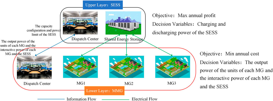
FIGURE 2. Schematic diagram of the dual-layer optimization model.

4.1 Upper layer model

4.1.1 Objective function

The optimization aim is meant to maximize the annual profit of the SESS, considering the construction investment and operation and maintenance costs, and the expression of the objective function is as follows:

$\max C_{\text{SESS}}={\displaystyle \sum _{i=1}^N\left[D_i\cdot \left(C{}_{\text{SESS,s,}i}-C{}_{\text{SESS,b,}i}+C{}_{\text{serve,}i}-C_{\text{inv,}i}\right)\right]}(9)$

where N denotes the type of typical days in a year, D_i denotes the number of days included on the i-th typical day in a year, C_SESS,s,i and C_SESS,b,i denote the SESS’ revenue from electricity sales and purchased electricity expenses on the i-th typical day, respectively, C_serve,i denotes the service change by the SESS to the MMGs on the i-th typical day, and C_inv,i denotes the investment and operation and maintenance costs of the SESS on the i-th typical day. The income and cost models of the SESS are as follows.

(1) Income of electricity sold to the MMGs on the i-th typical day

$C_{\text{SESS,s,}i}={\displaystyle \sum _{a=1}^A{\displaystyle \sum _{t=1}^T\left(\alpha \left(t\right)P_{\text{SESS,s,}i,a}(t)\mathrm{\Delta }t\right)}}(10)$

where A denotes the number of MGs; α(t) denotes the price of electricity sold by the MMGs in the time t; P_SESS,s,i,a(t) denotes the electricity sold to the MG a under Typical Day i by the SESS; T denotes the dispatch period, taken as 24h; and Δt denotes the interval duration of dispatch, taken as 1h.

(2) Cost of electricity bought from the MMGs on the i-th typical day

$C_{\text{SESS,b,}i}={\displaystyle \sum _{a=1}^A{\displaystyle \sum _{t=1}^T\left[\beta \left(t\right)P_{\text{SESS,b,}i,a}\left(t\right)\mathrm{\Delta }t\right]}}(11)$

where β(t) denotes the price of electricity bought from the MMGs in the time t and P_SESS,b,i,a(t) denotes the electricity purchased from the MG a under Typical Day i by the SESS.

(3) Service charges to the MMGs on the i-th typical day

$C_{\text{serve,}i}={\displaystyle \sum _{a=1}^A{\displaystyle \sum _{t=1}^T\left[\delta \left(t\right)\left(P_{\text{SESS,s,}i,a}\left(t\right)+P_{\text{SESS,b,}i,a}\left(t\right)\right)\mathrm{\Delta }t\right]}}(12)$

where δ(t) denotes the service charge received per unit of power for the interaction between the SESS and MMGs during the period t.

(4) Cost of investment, operation, and maintenance on the i-th typical day, without considering the effects of economic development and inflation

$C_{\text{inv,}i}=\frac{{\lambda }_{\text{P}}{P}_{\text{SESS}}^{\max }+{\lambda }_{\text{E}}{E}_{\text{SESS}}^{\max }}{T_E}+M_{\text{SESS}}(13)$

where λ_P and λ_E denote the power cost and capacity cost of the SESS, respectively; $P_{\text{SESS}}^{\max }$ and $E_{\text{SESS}}^{\max }$ denote the power limit and capacity limit of the SESS, respectively; T_E denotes the lifetime of the SESS; and M_SESS denotes the daily maintenance cost of the SESS.

4.1.2 Constraints

(1) Charging and discharging inherent constraints

$\{\begin{array}{l}{E}_{\text{SESS}}\left(0\right)=E_{\text{SESS}}\left(24\right)=20\%E_{\text{SESS}}^{\max },\\ 10\%E_{\text{SESS}}^{\max }\le E_{\text{SESS}}\left(t\right)\le 90\%E_{\text{SESS}}^{\max },\\ E_{\text{SESS}}\left(t\right)=E_{\text{SESS}}(t-1)+\left({\eta }_{\text{char}}{P}_{\text{char}}\left(t\right)-\frac{1}{{\eta }_{\text{dis}}}{P}_{\text{dis}}\left(t\right)\right)\mathrm{\Delta }t,\\ 0\le P_{\text{char}}\left(t\right)\le U_{\text{char}}\left(t\right)P_{\text{char}}^{\max },\\ 0\le P_{\text{dis}}\left(t\right)\le U_{\text{dis}}\left(t\right)P_{\text{dis}}^{\max },\\ U_{\text{char}}\left(t\right)+U_{\text{dis}}\left(t\right)\le 1,\end{array}(14)$

where E_SESS(t) indicates the storage capacity of the SESS in the period t; η_char and η_dis indicate the charging and discharging efficiency of the energy storage system; P_char(t) and P_dis(t) indicate the charging and discharging power of the SESS in the period t; E_SESS(0) and E_SESS(24) indicate the storage energy of the SESS at the beginning and the end of the dispatching cycle, respectively; $E_{\text{SESS}}^{\text{max}}$ indicates the maximum stored energy of the SESS; $P_{\text{char}}^{\text{max}}$ and $P_{\text{dis}}^{\text{max}}$ indicate the upper limit of charging and discharging power of the energy storage system, respectively; and U_char(t) and U_dis(t) ensure that the energy storage system can only be charged or discharged at the same moment during the scheduling cycle.

(2) Power and capacity limit constraints

$P_{\text{SESS}}^{\max }=\theta \cdot E_{\text{SESS}}^{\max }(15)$

where θ denotes the relative coefficient of power to the capacity limit of the SESS.

4.2 Lower layer model

This paper models each device in the MG and then optimizes the power output of each unit of the MMG-integrated energy system, the interactive power with the SESS, the consumption of the WT and PV power, and carbon emissions while considering the carbon trading mechanism and demand response.

4.2.1 Equipment output model

(1) Gas turbine (GT)

$P_{\text{GT,}i,a}\left(t\right)=P_{\text{GTI,}i,a}\left(t\right)\cdot {\eta }_{\text{GT}}(16)$

where P_GT,i,a(t) denotes the electrical power output from the GT of the MG a under Typical Day i in the time t; P_GTI,i,a(t) denotes the natural gas power input to the GT; and η_GT denotes the electrical conversion efficiency of the GT.

(2) Gas boiler (GB)

$P_{\text{GB},i,a}\left(t\right)=P_{\text{GBI},i,a}\left(t\right)\cdot {\eta }_{\text{GB}}(17)$

where P_GB,i,a(t) denotes the heating power output from the GB of the MG a under Typical Day i in the time t; P_GBI,i,a(t) denotes the natural gas power input to the GB; and η_GB denotes the heating conversion efficiency of the GB.

(3) Absorption chiller (AC)

$P_{\text{AC,}i,a}\left(t\right)=P_{\text{GT,}i,a}\left(t\right)\cdot {\gamma }_{\text{GT}}\cdot {\eta }_{\text{cooling}}\cdot R_{\text{AC}}(18)$

where P_AC,i,a(t) denotes the cooling power output from the AC of the MG a under Typical Day i in the time t; ϒ_GT denotes the thermoelectric ratio of the GT; η_cooling denotes the efficiency of the waste heat of the GT for cooling; and R_AC denotes the energy efficiency ratio of the AC.

(4) Electric chiller (EC)

$P_{\text{EC,}i\text{,}a}\left(t\right)=P_{\text{ECI,}i\text{,}a}\left(t\right)\cdot R_{\text{EC}}(19)$

where P_EC,i,a(t) denotes the cooling power output of the EC of the MG a under Typical Day i in the time t; P_ECI,i,a(t) denotes the electrical power input to the EC; and R_EC is the energy efficiency ratio of the EC.

(5) Heat exchange facility (HEF)

$P_{\text{HEF,}i\text{,}a}\left(t\right)=P_{\text{GT,}i\text{,}a}\left(t\right)\cdot {\gamma }_{\text{GT}}\cdot {\eta }_{\text{heating}}\cdot {\eta }_{\text{HEF}}(20)$

where P_HEF,i,a(t) is the heating power output of the HEF of the MG a under Typical Day i in the time t; η_heating is the proportion of waste heat from the GT used for heat production; and η_HEF is the efficiency of the HEF.

4.2.2 Ladder-type carbon trading mechanism based on the dynamic incentive coefficient

The relevant government departments award a specified reward when the overall carbon emissions of each unit in the integrated energy system are less than the free allotted carbon emission permit. In order to study the effects of different reward coefficients on carbon trading costs, this paper sets a dynamic incentive coefficient based on the ladder-type carbon trading mechanism (Qin et al., 2018; Zhang X. et al., 2020). The conventional carbon trading mechanism does not consider the equivalent carbon emissions generated by purchased electricity. Because purchased electricity may originate from thermal power units, this paper calculates the percentage of thermal power in the distribution network. It then calculates the carbon emissions generated by purchased electricity, thus quantifying the carbon emissions of purchased electricity. Thermal power, wind power, and hydropower are the primary sources of power for the examined regional grid. According to the year-over-year data of the region’s installed capacity, the percentage of thermal power generation (Gen) in the electricity distribution network during the dispatch period is ζ(t), as shown in Figure 3.

FIGURE 3

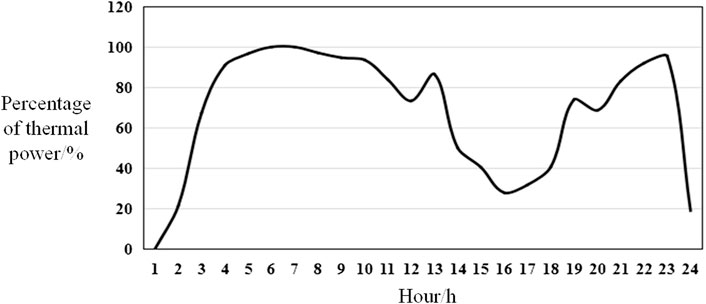
FIGURE 3. Percentage of thermal power in the electricity distribution network during the dispatch period.

The detailed calculation models of carbon trading mechanism are as follows:

$\{\begin{array}{l}{E}_{\text{GT0,}i}={\sigma }_{\text{h}}{\displaystyle \sum _{a=1}^A{\displaystyle \sum _{t=1}^T\left(\varphi \cdot P_{\text{GT,}i\text{,}a}\left(t\right)\mathrm{\Delta }t\right),}}\\ E_{\text{GB0,}i}={\sigma }_{\text{h}}{\displaystyle \sum _{a=1}^A{\displaystyle \sum _{t=1}^T\left(P_{\text{GB,}i\text{,}a}\left(t\right)\mathrm{\Delta }t\right)}},\\ E_{\text{Gen0,}i}={\sigma }_{\text{p}}{\displaystyle \sum _{a=1}^A{\displaystyle \sum _{t=1}^T\left(\zeta \left(t\right)\cdot P_{\text{grid},i\text{,}a}\left(t\right)\mathrm{\Delta }t\right)}},\\ E_{\text{L,}i}=E_{\text{GT0,}i}+E_{\text{GB0,}i}+E_{\text{Gen0,}i},\end{array}(21)$

where E_GT0,i, E_GB0,i, and E_Gen0,i denote the carbon emission allowances of the GT, the GB, and Gen on the i-th typical day, respectively; E_L,i denote the total carbon emission allowances; σ_h denotes the carbon emission allowances per unit of heat generation; ϕ denotes the conversion factor of electricity into heat; and σ_p denotes the carbon emission allowances per unit of electricity generation.

$\{\begin{array}{l}{E}_{\text{GT,}i}={\displaystyle \sum _{a=1}^A{\displaystyle \sum _{t=1}^T{a}_1{P}_{\text{GT,}i\text{,}a}^2\left(t\right)+b_1{P}_{\text{GT,}i\text{,}a}\left(t\right)+c_1,}}\\ E_{\text{GB,}i}={\displaystyle \sum _{a=1}^A{\displaystyle \sum _{t=1}^T{a}_2{P}_{\text{GB,}i\text{,}a}^2\left(t\right)+b_2{P}_{\text{GB,}i\text{,}a}\left(t\right)+c_2,}}\\ E_{\text{GT,}i}={\displaystyle \sum _{a=1}^A{\displaystyle \sum _{t=1}^T{a}_3{\left(\zeta \left(t\right)P_{\text{Gen,}i\text{,}a}\left(t\right)\right)}^2+b_3\left(\zeta \left(t\right)P_{\text{Gen,}i\text{,}a}\left(t\right)\right)+c_3,}}\\ E_{\text{P,}i}=E{}_{\text{GT,}i}+E{}_{\text{GB,}i}+E_{\text{Gen,}i},\end{array}(22)$

where E_GT,i, E_GB,i, and E_Gen,i denote the actual carbon emissions of the GT, the GB, and Gen on the i-th typical day, respectively; E_P,i denote the total actual carbon emissions; and a_i, b_i, and c_i (i = 1,2,3) denote the carbon emission factors of the GT, the GB, and Gen, respectively.

$C_{{\text{CO}}_2,i}=\{\begin{array}{c}-c\left(1+2\rho \right)\left(E_{\text{L},i}-\omega -E_{\text{P},i}\right),\\ E_{\text{P},i}\le E_{\text{L},i}-\omega \\ -c\left(1+2\rho \right)\omega -c\left(1+\rho \right)\left(E_{\text{L},i}-E_{\text{P},i}\right),\\ E_{\text{L},i}-\omega <E_{P,i}\le E_{\text{L},i}\\ c\left(E_{\text{P},i}-E_{\text{L},i}\right),\\ E_{\text{L},i}<E_{\text{P},i}\le E_{\text{L},i}+\omega \\ c\omega +c\left(1+\gamma \right)\left(E_{\text{P},i}-E_{\text{L},i}-\omega \right),\\ E_{L,i}+\omega <E_{\text{P},i}\le E_{\text{L},i}+2\omega \\ c\left(2+\gamma \right)\omega +c\left(1+2\gamma \right)\left(E_{\text{P},i}-E_{\text{L},i}-2\omega \right),\\ E_{\text{L},i}+2\omega <E_{\text{P},i}\le E_{\text{L},i}+3\omega \\ c\left(3+3\gamma \right)\omega +c\left(1+3\gamma \right)\left(E_{\text{P},i}-E_{\text{L},i}-3\omega \right),\\ E_{\text{L},i}+3\omega <E_{\text{P},i},\end{array}(23)$

where c denotes the unit price of carbon trading in the market, taken as 0.27 RMB/kg, ϒ denotes the rising range of carbon trading price for each step type, taken as 25%, ω denotes the length of carbon emission interval, taken as 500kg, and ρ denotes the dynamic carbon trading incentive coefficient. When the total actual carbon emissions of the MMGs are smaller than the total carbon emission allowances, the relevant government departments give the incentive allowance. The value of the dynamic incentive coefficient determines the carbon trading cost from a macroscopic point of view.

4.2.3 Objective function

The lower optimization objective is the lowest operating cost of the MMG-integrated energy system, considering the promotion of new energy consumption and low-carbon operation. The total cost includes the income of electricity sold to the SESS, the cost of electricity bought from the SESS, the service charges, the cost of electricity bought from the distribution grid, the cost of gas purchased, the penalty cost of abandoning the WT and PV power, and the carbon trading cost, so the objective function is integrated as follows:

$\min C_{\text{MMGs}}={\displaystyle \sum _{i=1}^N\left[D_i\cdot \left(C_{\text{SESS,s,}i}-C_{\text{SESS,b,}i}+C_{\text{serve,}i}+C_{\text{grid,}i}+C_{\text{gas,}i}+C_{{\text{CO}}_2,i}+C_{\text{aban},i}\right)\right]}(24)$

where N denotes the type of typical days in a year, D_i denotes the number of days for the i-th typical day in a year, C_SESS,s,i and C_SESS,b,i denote the cost of electricity purchased from the SESS and the income of electricity sold to the SESS on the i-th typical day, C_serve,i denotes the service charges paid by the MMGs to the SESS, C_grid,i denotes the cost of electricity purchased from the distribution grid, C_gas,i denotes the cost of gas for the GT and GB, C_CO2,i denotes the cost of carbon trading, and C_loss,i denotes the penalty cost of abandoning the WT and PV power. Among them, C_SESS,s,I, C_SESS,b,I, and C_CO2,i are calculated according to Eq.10, 11, and Eq. 23, and the rest of the costs are calculated as follows.

(1) Cost of electricity purchased from the distribution grid on the i-th typical day

$C_{\text{grid,}i}={\displaystyle \sum _{a=1}^A{\displaystyle \sum _{t=1}^T\left[c_{\text{grid}}\left(t\right)\cdot P_{\text{grid,}i\text{,}a}\left(t\right)\cdot \mathrm{\Delta }t\right]}}(25)$

where c_grid(t) denotes the time-of-day tariff for electricity purchased from the distribution grid and P_grid,i,a(t) denotes the electricity purchased from the distribution grid by the MG a under Typical Day i in the time t.

(2) Cost of purchasing gas on the i-th typical day

$C_{\text{grid,}i}={\displaystyle \sum _{a=1}^A{\displaystyle \sum _{t=1}^T\left[c_{\text{grid}}\left(t\right)\cdot P_{\text{grid,}i\text{,}a}\left(t\right)\cdot \mathrm{\Delta }t\right]}}(26)$

where L_NG denotes the calorific value of gas and is taken as $9.6\left(\text{kW}\cdot \text{h}\right)/{\text{m}}^3$ and c_gas denotes the price per unit volume of gas and is taken as 3 RMB/m³.

(3) Cost of the WT and PV power abandonment penalty on the i-th typical day

$C_{\text{aban,}i}={\displaystyle \sum _{a=1}^A{\displaystyle \sum _{t=1}^T\left\{{\mu }_{\text{w}}\left[P_{\text{wI,}i\text{,}a}\left(t\right)-P_{\text{w,}i\text{,}a}\left(t\right)\right]+{\mu }_{\text{PV}}\left[P_{\text{PVI,}i\text{,}a}\left(t\right)-P_{\text{PV,}i\text{,}a}\left(t\right)\right]\mathrm{\Delta }t\right\}}}(27)$

where P_wI,i,a(t) and P_w,i,a(t) denote the wind power input and the wind power consumed by the MG a under Typical Day i in the time t, respectively; P_PVI,i,a(t) and P_PV,i,a(t) denote the PV power input and the PV power consumed by the MG a under Typical Day i in the time t, respectively; and µ_w and µ_PV are the penalty coefficient of the WT and PV power abandonment, respectively.

4.2.4 Constraints

Lower level optimization constraints include system operation constraints, operational constraints of each generation equipment, power interaction constraints, user satisfaction constraints, constraints of power interacting with the SESS, and constraints of WT and PV power consumption, which are expressed as follows.

(1) Constraints on power balance

$\{\begin{array}{l}{P}_{\text{GT,}i\text{,}a}\left(t\right)+P_{\text{w,}i\text{,}a}\left(t\right))+P_{\text{PV,}i\text{,}a}\left(t\right)+P_{\text{grid,}i\text{,}a}\left(t\right)+P_{\text{SESS,s,}i\text{,}a}\left(t\right)-P_{\text{SESS,b,}i\text{,}a}\left(t\right)=P_{\text{el,}i\text{,}a}\left(t\right),\\ P_{\text{GB,}i\text{,}a}\left(t\right)+P_{\text{HEF,}i\text{,}a}\left(t\right)=P_{\text{hl,}i\text{,}a}\left(t\right),\\ P_{\text{EC,}i\text{,}a}\left(t\right)+P_{\text{AC,}i\text{,}a}\left(t\right)=P_{\text{cl,}i\text{,}a}\left(t\right),\end{array}(28)$

where P_el,i,a(t), P_hl,i,a(t), and P_cl,i,a(t) denote the electrical load, heating load, and cooling load power of the MG a under Typical Day i in the period t, respectively.

(2) Constraints on equipment output

$\{\begin{array}{l}{P}_{\text{GT}}^{\text{min}}\le P_{\text{GT,}i\text{,}a}\left(t\right)\le P_{\text{GT}}^{\text{max}},\\ P_{\text{GT}}^{\text{down}}\le P_{\text{GT,}i\text{,}a}\left(t\right)-P_{\text{GT,}i\text{,}a}\left(t-1\right)\le P_{\text{GT}}^{\text{up}},\\ P_{\text{GB}}^{\min }\le P_{\text{GB,}i\text{,}a}\left(t\right)\le P_{\text{GB}}^{\max },\\ P_{\text{GB}}^{\text{down}}\le P_{\text{GB},i\text{,}a}\left(t\right)-P_{\text{GB},i\text{,}a}\left(t-1\right)\le P_{\text{GB}}^{\text{up}},\\ P_{\text{AC}}^{\min }\le P_{\text{AC,}i\text{,}a}\left(t\right)\le P_{\text{AC}}^{\max },\\ P_{\text{EC}}^{\min }\le P_{\text{EC,}i\text{,}a}\left(t\right)\le P_{\text{EC}}^{\max },\\ P_{\text{HX}}^{\text{min}}\le P_{\text{HX},i,a}\left(t\right)\le P_{\text{HX}}^{\text{max}},\\ P_{\text{grid}}^{\min }\le P_{\text{grid,}i\text{,}a}\left(t\right)\le P_{\text{grid}}^{\max },\end{array}(29)$

where $P_{\text{X}}^{\text{max}}$ and $P_{\text{X}}^{\text{min}}$ represent the upper and lower power limits of X, respectively, and $P_{\text{X}}^{\text{up}}$ and $P_{\text{X}}^{\text{down}}$ represent the upper and lower limits of climbing power of X, respectively.

(3) Constraints on users’ satisfaction with the way of using electricity (Eq. 8)

4.3 Solving method

In the dual-layer optimization model of the MMG-integrated energy system constructed in this paper, the upper layer problem is a non-linear non-convex optimization problem and the lower layer is a convex optimization problem. Because the traditional solution approach for this problem is to solve it by converting the dual-layer into a single-layer, this study uses the KKT method to convert the lower layer model into the upper layer constraints. In addition, due to the difficulty of handling non-linear constraints, some of them are reduced to linear constraints using the Big M approach without sacrificing solution accuracy. The mixed-integer linear programming issue posed by the converted single-layer model can be solved using the Gurobi solver. Figure 4 depicts the general solution idea diagram for this article. In order to obtain scenic output curves for four typical days of the year, clustering was performed using the K-means method based on historical data of the region, which will not be described in detail here.

FIGURE 4

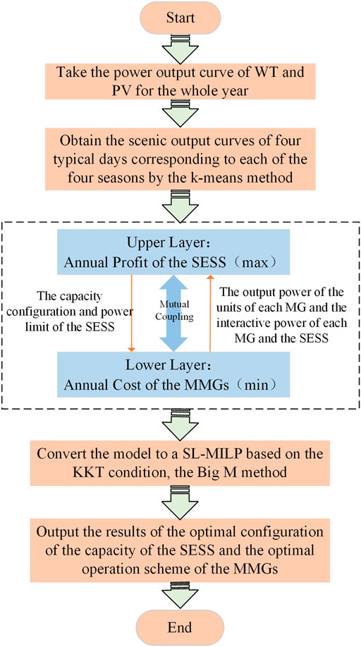
FIGURE 4. Solving flowchart.

The lower model is transformed into the upper model using restrictions on the Lagrangian function and the KKT condition. Because the original model’s lower layer problem is a min problem, the product of multipliers and restrictions in the Lagrangian relaxation must be less than or equal to 0.

Due to the non-linear inequality requirements in the single-layer transformed model, there is a scenario of multiplication of two continuous variables that are extremely difficult to solve. As a result, the Big M approach is used to linearize the non-linear inequalities in this study.

The generated single-layer optimization model corresponds to the mixed-integer linear optimization problem after KKT conversion and linearization. The arithmetic simulation is modeled using the Yalmip optimization tool in MATLAB R2018b environment and solved using the solver Gurobi.

5 Case study

5.1 Case parameters and scenario settings

The research object is a real MMG-integrated energy system, which includes three independently operated combined cooling, heating, and power MGs: MG1, MG2, and MG3. The electricity price of each MG from the distribution grid is the peak-to-valley tariff, and the electricity purchase and sale prices between each MG and the SESS in Wu et al. (2021b) are introduced. The maximum power of each MG interacting with the distribution grid in the period t is 3000 kW. The maximum power of each MG interacting with the SESS in the period t is 4000 kW. For the time being, electricity interaction between MGs has not been considered since the emergence of third-party SESS.

The three MGs for 1 year’s electrical, heating, and cooling load curves are clustered and selected using the K-means method. The electrical, heating, and cooling load curves for four typical days corresponding to four seasons of the year are obtained, as shown in Wu et al. (2021b). The dispatch period T is set to 24 h, the scheduling interval length Δt is 1 h, and each type of typical day in a year corresponds to 91 days. Each of the three MGs has 200 integrated energy users. The exact parameters of transportable non-interruptible equipment, such as electricvehicles are shown in Li et al. (2020).

Three types of scenarios were created to examine and compare the influence of optimal energy storage and demand response configurations on system operation:

Scenario 1: For the MMG-integrated energy system, optimized dispatching is conducted without considering demand response.

Scenario 2: Based on scenario 1, the scheduling of the MMG-integrated energy system is optimized without considering energy storage access but considering demand response.

Scenario 3: The capacity of SESS is optimally assigned without regard for the demand response, and optimal scheduling for the MMG-integrated energy system is executed.

Scenario 4: The capacity of SESS is efficiently distributed while considering the demand response, and optimal scheduling is achieved for the MMG-integrated energy system using the dual-layer optimization model developed in this research.

5.2 Efficiency analysis of the solving method

According to Table 1, it can be concluded that the average solving time is relatively fast and the gap also meets the requirements.

TABLE 1

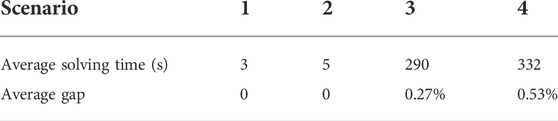
TABLE 1. Comparison of the average solving time and gap for the four scenarios.

5.3 Analysis of case results

5.3.1 Comprehensive optimization effect comparison of different scenarios

Based on the solution results, the annual profit of the SESS, the annual operation cost of the MMGs, and the annual amount of abandoned WT and PV electricity are compared for the four scenarios, as shown in Table 2. Given that the load of the multi-microgrid varies on different typical days and the scenery power varies, the specific cost and cost of the MMGs are compared and studied independently on a typical spring day, as shown in Table 3.

TABLE 2

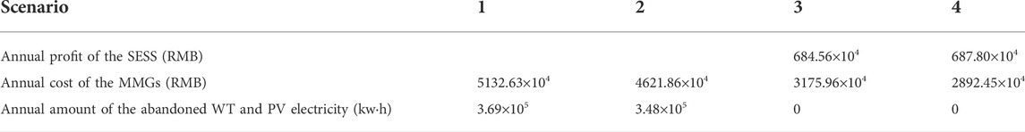
TABLE 2. Comparison of the annual profit of the SESS, annual cost of the MMGs, and annual amount of the abandoned WT and PV electricity.

TABLE 3

TABLE 3. Comparison of costs of each of the four scenarios of the MMGs on a typical day in spring.

The following conclusions can be drawn by comparing the data results in Tables 1, 2.

(1) Scenario 4 reduces the annual amount of abandoned WT and PV electricity of the MMG-integrated energy system to 0 and the annual operation cost by 2240.18 × 10⁴ and 1956.67 × 10⁴ RMB, respectively, scenarios 1 and 2. It can be seen that the SESS promotes full utilization of the WT and PV power while lowering total cost. Although purchasing power from the SESS exceeds the profits from power sales, a complete cost-benefit analysis demonstrates that the system provides more comprehensive benefits than the cost of power interaction with the SESS.

(2) Scenario 4 introduces demand response with controllable load from the operation level, which takes into account the independent transfer and adjustment of electrical, heating, and cooling loads on the demand side and improves system operation flexibility so that the annual cost of the MMGs is reduced by 283.51 × 10⁴ RMB. The annual profit of the SESS is increased by 32,400 RMB, while all costs of the MMGs are reduced. In a broader sense, the dual flexibility of considering shared energy storage and demand response simultaneously increases the annual profit of the SESS. It lowers the operation cost of the MMGs, resulting in “win–win” economic benefits for the SESS and MMGs.

(3) The carbon transaction cost of scenario 4 is reduced by 3996.00, 3976.46, and 245.24 RMB when compared to that of scenarios 1, 2, and 3, respectively, because the MMGs reduce the output of GTs, GBs, and other units by interaction of electricity with the SESS, thereby reducing carbon emissions. After considering demand response, each MG can more reasonably allocate electricity, heat, and cold to realize full utilization of energy within each MG, reduce energy interaction with external energy networks, and reduce carbon emissions. The proposed dual-layer optimization methodology can improve the environmental advantages of the MMG-integrated energy system.

5.3.2 Impact of SESS access on the system

The electrical loads for scenarios 2 and 4 under Spring Typical Day are shown in Figures 5, 6. In Figure 6, it is clear that, after accounting for the SESS access of the three MGs throughout the dispatching cycle, the abandoned power falls to zero. During 10–12 h, the distribution grid electricity price is lower than the SESS electricity price. Thermal power in the grid accounts for a relatively low cost of carbon trading, so MG 1 purchases power from the grid to meet the electric load demand. Because wind power is more extensive throughout the dispatching cycle, MG 1 sells the new energy power that cannot be consumed by the SESS. MG 2 uses just the PV power and no WT power. During 0–9 h, the PV power is low, and MG 2 purchases power from the SESS and the grid to meet the electric load demand; during 10–12 h, the PV power gradually increases, and MG 2 changes its operation state to selling power to the SESS, reaching a peak at 12 h. After 14 h, the PV power gradually decreases, and MG 2 generally shows that it purchases power from the SESS. Because MG 3 has reduced WT and PV output during the dispatching cycle, it must acquire power from the SESS throughout the dispatching cycle. The sum of power purchased from and sold to the SESS in microgrids 1, 2, and 3 is balanced throughout the dispatching cycle. The cooling and heating loads under Spring Typical Day balance diagrams for scenarios 2 and 4 are shown in Appendix Tables A2 and A3.

FIGURE 5

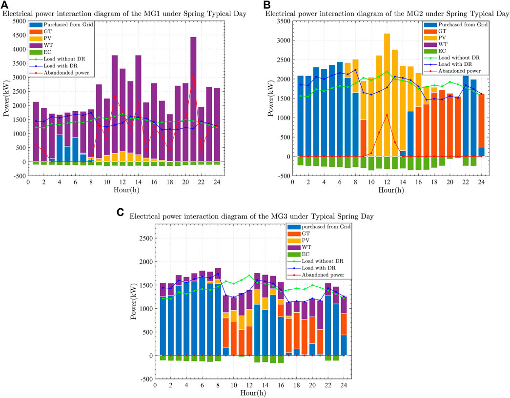
FIGURE 5. Electrical power interaction diagrams under Spring Typical Day in scenario 2: (A) MG1, (B) MG2, and (C) MG3.

FIGURE 6

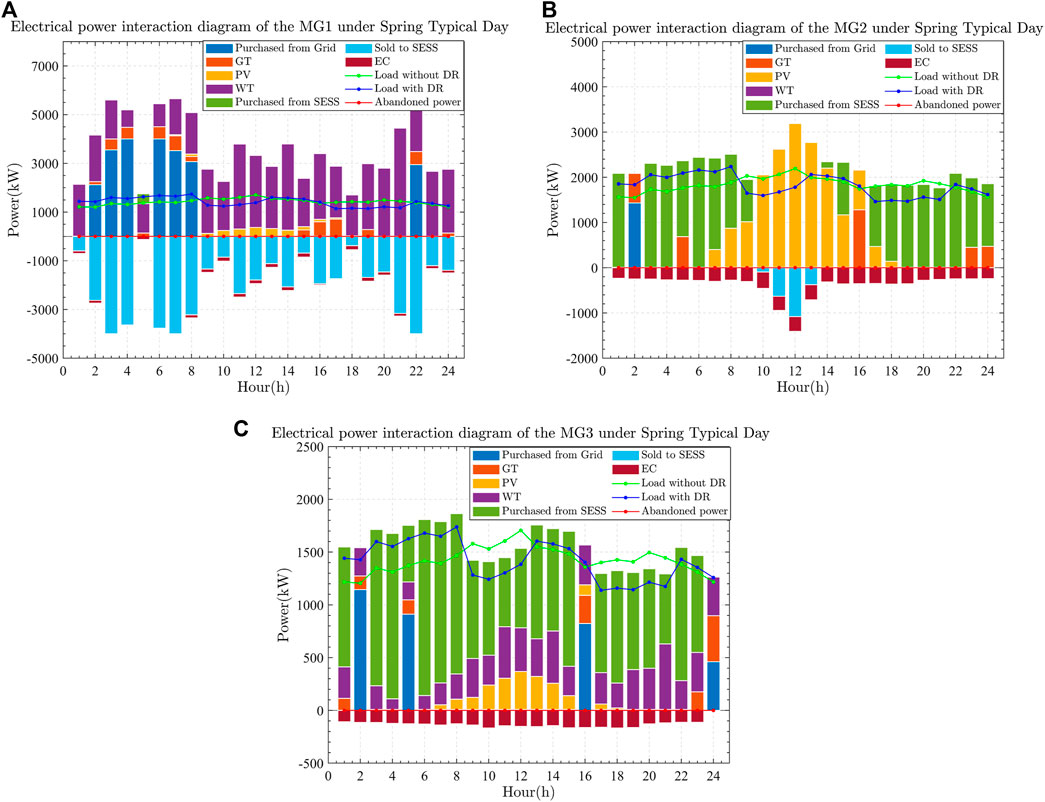
FIGURE 6. Electrical power interaction diagrams under Spring Typical Day in scenario 4: (A) MG1, (B) MG2, and (C) MG3.

5.3.3 Impact of demand response on the system

Table 4 and Figure 7 show the capacity allocation and power limits of the SESS in scenarios 3 and 4 under Spring Typical Day. In scenario 4, compared to scenario 3, the SESS charging and discharging power limits increase daily, as does the allocated capacity; on an hourly basis, the charging and discharging power curve and capacity allocation curve of the SESS fluctuate more. Because after fully considering the demand response on the load side, integrated energy users’ energy use is more reasonable, and the internal consumption capacity of the MMG-integrated energy system is improved. The cost of each energy use is reduced, allowing the SESS to maximize its economic benefits by increasing charging and discharging power and allocating more capacity.

TABLE 4

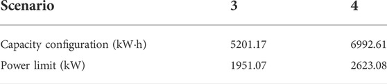
TABLE 4. Capacity configuration and power limit of the SESS under Spring Typical Day.

FIGURE 7

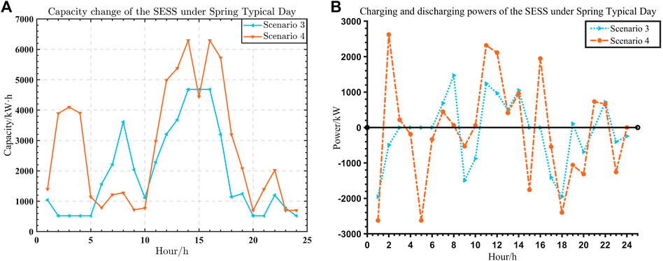
FIGURE 7. Comparison of the capacity change and charging and discharging power of the SESS under Spring Typical Day between scenarios 3 and 4: (A) capacity change; (B) charging and discharging power.

Figure 8 depicts a comparison of the electric loads of the MMGs under Spring Typical Day scenarios 3 and 4. After considering the demand response on the load side, the integrated energy users of the three MGs are guided by the time-of-use tariff to shift part of the electrical load to the period with a lower tariff. In contrast, the cooling and heating loads of the multiple microgrids are optimally adjusted without affecting customer comfort. All three microgrids can achieve “de-peaking” which enables the time-division scheduling and relieves the operating pressure of the three MGs.

FIGURE 8

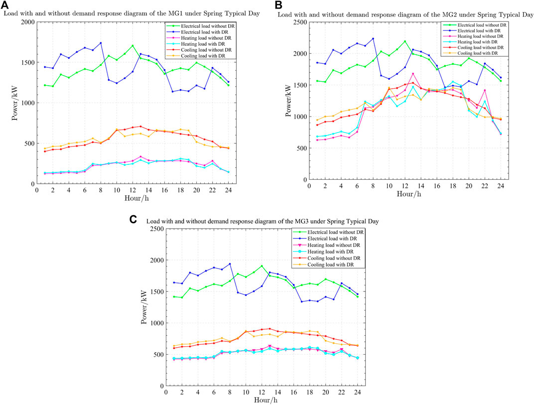
FIGURE 8. Comparison of the electrical loads under Spring Typical Day between scenarios 3 and 4: (A) MG1, (B) MG2, and (C) MG3.

5.3.4 Impact of synergy between the SESS and demand response on the system

The comparison results of scenario 4 with the rest of the scenarios and the above analysis show that the synergy of load and storage flexibility resources can make load fluctuations more compatible with new energy fluctuations. Energy storage plays a role in consuming abandoned WT and PV power entirely through reasonable capacity allocation. Multiple microgrids enjoy storage charging and discharging services while reducing storage construction investment through storage charging and discharging services. The demand response mechanism guides each microgrid to allocate electrical, heating, and cooling loads rationally. Furthermore, it realizes full energy utilization within each microgrid, reducing energy interaction with external energy networks, the output of GTs and GBs, and carbon emissions while using resources rationally, thus lowering the system’s total operating cost. The MMG-integrated energy system’s synergy of energy storage and demand response can be seen to balance the economy and low-carbon operation.

5.3.5 Analysis of the role of the carbon trading mechanism considering the dynamic incentive coefficient

Figure 9A depicts the curves of the upper optimization model’s profit of the SESS and the lower optimization model’s variation of the total cost of the MMGs with the dynamic incentive coefficient. Because the model in this paper does not consider equipment with high carbon emissions, such as thermal power units, the actual carbon emissions of the MMGs are always less than the initial carbon emission allowance. Thus, the carbon trading cost is always negative. The government rewards the MMGs with a specific allowance, lowering the total cost and achieving low-carbon optimized operation. When the dynamic incentive coefficient increases from 0.1 RMB/kg to 0.4 RMB/kg, the absolute value of the system’s carbon trading cost shows a linear growth trend. The total cost gradually decreases, while the profit of the SESS increases because the MMGs prefer to interact with the SESS to obtain electric power. When the dynamic incentive coefficient rises above 0.4 RMB/kg, the profit of the SESS and the total cost of the MMGs remain stable.

FIGURE 9

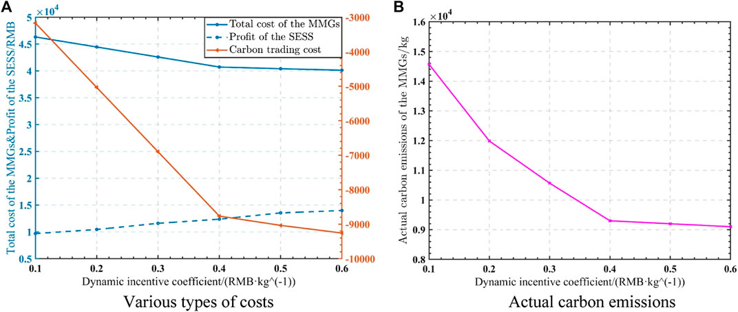
FIGURE 9. Curves of various types of costs and actual carbon emissions with the dynamic incentive coefficient: (A) various types of costs; (B) actual carbon emissions.

As shown in Figure 9B, as the dynamic incentive coefficient increases from 0.1 RMB/kg to 0.4 RMB/kg, the carbon emissions of the MMGs noticeably decrease. However, when the dynamic incentive coefficient exceeds 0.4 RMB/kg, the actual carbon emissions of the MMGs remain nearly unchanged because the MMGs have almost reached equilibrium. The power interaction tends to be in the steady-state, so the carbon trading price has less influence on its electric power interaction. It is not practical to continue increasing the dynamic incentive coefficient, so it should be 0.4 RMB/kg. Based on this paper’s findings, the incentive coefficient’s contribution above a specific value to reducing carbon trading costs becomes increasingly tiny, indicating that an optimal incentive coefficient exists. It can be seen that the model proposed in this paper can serve as a valuable reference for determining a dynamic incentive coefficient.

6 Conclusion

A configuration-dispatch dual-layer optimization model of an MMG-integrated energy system with SESS access and demand response is proposed in this paper. The following conclusions are drawn from simulation results of arithmetic cases under different scenarios using an existing MMG-integrated energy system as the research object:

(1) Accessing shared energy storage in the MMG-integrated energy system can achieve total WT and PV power consumption through the power interaction between the MMGs and the SESS. It also minimizes the total cost of the MMGs while maximizing the annual profit of the SESS, reduces the carbon emission of the MMGs, and realizes the low-carbon operation of the MMG-integrated energy system.

(2) The introduction of demand response has facilitated the time-domain deployment of electrical, heating, and cooling loads realized (“peak-shaving and valley-filling” loads). It also uses flexible resources to improve the MMG-integrated energy system’s economy and low-carbon operation and relieve each MG’s operating pressure.

(3) The MMG-integrated energy system can achieve the dual goals of low carbon and economic operation after implementing a carbon trading mechanism. The total cost of the MMGs can be reduced by increasing the dynamic incentive coefficient. However, promoting low carbon is not apparent until the coefficient exceeds a specific value, so introducing a carbon trading mechanism and setting a suitable dynamic incentive coefficient are an effective means to realize the low-carbon operation of an integrated energy system.

(4) The joint operation of more MMGs will be investigated, and the solution efficiency of the proposed method will be verified in conjunction with practical application requirements.

Data availability statement

The datasets presented in this study can be found in online repositories. The names of the repository/repositories and accession number(s) can be found in the article/supplementary material.

Author contributions

KW and YL proposed the methodology, conducted the theoretical analysis as well as the simulation verification, and wrote the original draft, which was reviewed and edited by KW and RJ. XW, HD, and XM contributed to the supervision. All authors agreed to be accountable for the content of the work.

Funding

This research was supported by the Shaanxi Province Science and Technology Project (No. 2022JM-208) and the laboratory research project of State Grid Co., Ltd, Gansu Youth Science, and Technology program (21JR7RA745).

The authors declare that this study received funding from the laboratory research project of State Grid Co., Ltd., Gansu Youth Science and Technology program (21JR7RA745). The funder was not involved in the study design, collection, analysis, interpretation of data, the writing of this article or the decision to submit it for publication.

Conflict of interest

The author XM was employed by State Grid Gansu Electric Power Company.

The remaining authors declare that the research was conducted in the absence of any commercial or financial relationships that could be construed as a potential conflict of interest.

Publisher’s note

All claims expressed in this article are solely those of the authors and do not necessarily represent those of their affiliated organizations, or those of the publisher, the editors, and the reviewers. Any product that may be evaluated in this article, or claim that may be made by its manufacturer, is not guaranteed or endorsed by the publisher.

Abbreviations

AC, absorption chiller; DR, demand response; EC, electric chiller; GB, gas boiler; GT, gas turbine; HEF, heat exchange facility; IES, integrated energy system; MG, microgrid; MMGs, multi-microgrids; PV, photovoltaic; SESS, shared energy storage system; WT, wind turbine.

References

Fan, P., Ke, S., Yang, J., Li, Y., Xiao, J., and Xu, B. (2022). Load frequency coordinated control strategy of multi-microgrid based on improved MA-DDPG. Power Syst. Technol. 43 (10), 1–12. doi:10.13335/j.1000-3673.pst.2021.1918

CrossRef Full Text | Google Scholar

Gao, Y., and Ai, Q. (2021). Demand-side response strategy of multi-microgrids based on an improved co-evolution algorithm. CSEE J. Power Energy Syst. 7 (5), 903–910. doi:10.17775/CSEEJPES.2020.06150

CrossRef Full Text | Google Scholar

Gu, X., Wang, Q., Hu, Y., Zhu, Y., and Ge, Z. (2022). Distributed low-carbon optimal operation strategy of multi-microgrids integrated energy system based on Nash bargaining. Power Syst. Technol. 46 (04), 1464–1482. doi:10.13335/j.1000-3673.pst.2021.1967

CrossRef Full Text | Google Scholar

Guo, C., Wang, X., Zheng, Y., and Zhang, F. (2021). Optimal energy management of multi-microgrids connected to distribution system based on deep reinforcement learning. Int. J. Electr. Power & Energy Syst. 131, 107048. doi:10.1016/j.ijepes.2021.107048

CrossRef Full Text | Google Scholar

Li, J., Ma, G., Li, T., Chen, W., and Gu, Y. (2019). A Stackelberg game approach for demand response management of multi-microgrids with overlapping sales areas. Sci. China Inf. Sci. 62 (11), 212203. doi:10.1007/s11432-018-9814-4

CrossRef Full Text | Google Scholar

Li, P., Wu, D., Li, Y., Yin, Y., Fang, Q., and Chen, B. (2020). Multi-objective union optimal configuration strategy for multi-microgrid integrated energy system considering bargaining games. Power Syst. Technol. 44 (10), 3680–3688. doi:10.13335/j.1000-3673.pst.2020.0289

CrossRef Full Text | Google Scholar

Li, L. (2021a). Coordination between smart distribution networks and multi-microgrids considering demand side management: A trilevel framework. Omega 102, 102326. doi:10.1016/j.omega.2020.102326

CrossRef Full Text | Google Scholar

Li, X., Xie, S., Fang, Z., Li, F., and Cheng, S. (2021b). Optimal configuration of shared energy storage for multi-microgrid and its cost allocation. Electr. Power Autom. Equip. 41 (10), 44–51. doi:10.16081/j.epae.202110019

CrossRef Full Text | Google Scholar

Li, Z., Chen, S., Dong, W., Liu, P., Du, E., Ma, L., et al. (2021c). Low carbon transition pathway of power sector under carbon emission constraints. Proc. CSEE 41 (12), 3987–4001. doi:10.13334/j.0258-8013.pcsee.210671

CrossRef Full Text | Google Scholar

Liu, Y., Chen, X., Li, B., and Zhu, J. (2020). State of art of the key technologies of multiple microgrids system. Power Syst. Technol. 44 (10), 3804–3820. doi:10.13335/j.1000-3673.pst.2019.2157

CrossRef Full Text | Google Scholar

Qin, T., Liu, H., Wang, J., Feng, Z., and Fang, W. (2018). Carbon trading based low-carbon economic dispatch for integrated electricity-heat-gas energy system. Automation Electr. Power Syst. 42 (14), 8–13. doi:10.7500/AEPS20171220005

CrossRef Full Text | Google Scholar

Shuai, X., Ma, Z., Wang, X., Guo, H., and Zhang, H. (2022). Research on optimal operation of shared energy storage and integrated energy microgrid based on leader-follower game theory. Power Syst. Technol. 45 (10), 1–12. doi:10.13335/j.1000-3673.pst.2021.2191

CrossRef Full Text | Google Scholar

Shuai, X., Wang, X., Yuan, S., Chen, G., and Huang, Y. (2021). Design of multi-microgrid energy trading mechanism based on improved Nash bargaining method in electricity market environment. J. Xi’an Jiaot. Univ. 55 (11), 97–105. doi:10.7652/xjtuxb20211101

CrossRef Full Text | Google Scholar

Tan, C., Geng, S., Tan, Z., Wang, G., Pu, L., Guo, X., et al. (2021). Integrated energy system–Hydrogen natural gas hybrid energy storage system optimization model based on cooperative game under carbon neutrality. J. Energy Storage 38, 102539. doi:10.1016/j.est.2021.102539

CrossRef Full Text | Google Scholar

Wang, Y., Wang, X., Sun, Q., Zhang, Y., and Liu, Z. (2022). Multi-agent real-time collaborative optimization strategy for integrated energy system group based on energy sharing. Automation Electr. Power Syst. 46 (4), 56–65. doi:10.7500/AEPS20210511007

CrossRef Full Text | Google Scholar

Wang, Y., Xie, H., Sun, X., and Bie, Z. (2021). Day-ahead economic dispatch for electricity-heating integrated energy system considering incentive integrated demand response. Trans. China Electrotech. Soc. 36 (9), 1926–1934. doi:10.19595/j.cnki.1000-6753.tces.L90240

CrossRef Full Text | Google Scholar

Wu, J., Lou, P., Guan, M., Huang, Y., Zhang, W., and Cao, Y. (2021a). Operation optimization strategy of multi-microgrids energy sharing based on asymmetric Nash bargaining. Power Syst. Technol. 46 (4), 1–13. doi:10.13335/j.1000-3673.pst.2021.1590

CrossRef Full Text | Google Scholar

Wu, S., Li, Q., Liu, J., Zhou, Q., and Wang, C. (2021b). Bi-level optimal configuration for combined cooling heating and power multi-microgrids based on energy storage station service. Power Syst. Technol. 45 (10), 3822–3832. doi:10.13335/j.1000-3673.pst.2020.1838

CrossRef Full Text | Google Scholar

Wu, S., Liu, J., Zhou, Q., Wang, C., and Chen, Z. (2019). Optimal economic scheduling for multi-microgrid system with combined cooling, heating and power considering service of energy storage station. Automation Electr. Power Syst. 43 (10), 10–18. doi:10.7500/AEPS20181024001

CrossRef Full Text | Google Scholar

Xiang, Y., Wu, G., Shen, X., Ma, Y., Gou, J., Xu, W., et al. (2021). Low-carbon economic dispatch of electricity-gas systems. Energy 226, 120267. doi:10.1016/j.energy.2021.120267

CrossRef Full Text | Google Scholar

Xu, Q., Li, L., Cai, J., Luan, K., and Yang, B. (2018). Day-ahead optimized economic dispatch of CCHP multi-microgrid system considering power interaction among microgrids. Automation Electr. Power Syst. 42 (21), 36–44. doi:10.7500/AEPS20180417006

CrossRef Full Text | Google Scholar

Zhang, W., and Xu, Y. (2018). Distributed optimal control for multiple microgrids in a distribution network. IEEE Trans. Smart Grid 10 (4), 3765–3779. doi:10.1109/TSG.2018.2834921

CrossRef Full Text | Google Scholar

Zhang, X., Liu, X., and Zhong, J. (2020a). Integrated energy system planning considering a reward and punishment ladder-type carbon trading and electric-thermal transfer load uncertainty. Proc. Chin. Soc. Electr. Eng. 40 (19), 6132–6141. doi:10.13334/j.0258-8013.pcsee.191302

CrossRef Full Text | Google Scholar

Zhang, Y., Ai, Q., Wang, H., Li, Z., and Huang, K. (2020b). Bi-level distributed day-ahead schedule for islanded multi-microgrids in a carbon trading market. Electr. Power Syst. Res. 186, 106412. doi:10.1016/j.epsr.2020.106412

CrossRef Full Text | Google Scholar

Zhu, W., Luo, Y., Hu, B., Luo, H., Zhang, Y., Han, Y., et al. (2021). Optimized combined heat and power dispatch considering decreasing carbon emission by coordination of heat load elasticity and time-of-use demand response. Power Syst. Technol. 45 (10), 3803–3812. doi:10.13335/j.1000-3673.pst.2020.2121

CrossRef Full Text | Google Scholar