Abstract
Accurate forecasting of an electric load is vital in the effective management of a power system, especially in flourishing regions. A new hybrid model called logarithmic spiral firefly algorithm-support vector regression (LS-FA-SVR) is proposed to promote the performance of electric load forecasting. The new hybrid model is acquired by combining the support vector regression, firefly algorithm, and logarithmic spiral. Half-hourly electric load from five main regions (NSW, QLD, SA, TAS, and VIC) of Australia are used to train and test the proposed model. By comparing the model results with observed data on the basis of the root mean squared error (RMSE), mean absolute error (MAE), and mean absolute percent error (MAPE), the performance of the proposed hybrid model is the most outstanding among all the considered benchmark models. Hence, the results of this study show that the hybrid model LS-FA-SVR is preferable and can be applied successfully because of its high accuracy.
1 Introduction
As an integrated system that can optimize the allocation of energy resources according to the regional energy structure and energy reserves, an integrated energy system has become an important way to accelerate the global sustainable energy transformation. Accurate load forecasting not only plays a decisive role in the comprehensive planning, operation, management and cascade use of energy system but is also a key technology to promote the development of the energy market (Wang et al., 2018; Chen and Wang, 2021; Yang et al., 2022c). Hence, technology for the smart and efficient management of grid uncertainty has attracted research interest. In particular, load forecasting is a core factor of smart grid applications, such as demand response, as it can accurately predict the demand flexibility and potential problems in a grid. In addition, load forecasting can contribute to the efficient integration and wide allocation of distributed energy resources and their coordination to accommodate supply and demand (Kaur et al., 2016). Therefore, the prediction of the short-term load has become the chief task in power dispatching and power planning (Wu et al., 2021; Yang et al., 2022d).
However, high accuracy in predicting a short-term load is difficult to obtain because the electric load time series is complex and shows vacillating behavior with many variables considered. In order to deal with this problem, regression models, stochastic process models, and exponential smoothing are employed to forecast the electric load in traditional methods (Zhang et al., 2021, 2022b,a). However, the traditional methods scarcely acquire the complexity of the system. Hence, artificial intelligence approaches are extensively used to predict the power load, such as artificial neural networks, support vector machines, and nature-inspired meta-heuristic algorithms.
Among all the data mining techniques based on artificial intelligence, artificial neural networks have become hot techniques in the research of forecasting electric load. Yang et al. (2022a) developed a highly accurate short-term load forecasting method using non-linear auto-regressive artificial neural networks with exogenous multi-variable input. Yang et al. (2022b) presented a novel approach for short-term electrical load forecasting by the radial basis function neural networks, and the result showed that the application of neural networks in short-term load forecasting is encouraging. Wang et al. (2016) proposed an outstanding model based on a wavelet neural network to address the complex nonlinearities and uncertainties in forecasting the electric load, and the accuracy of the proposed model is better than the considered models. Yang et al. (2021b) proposed a new hybrid model to forecast electric load series with outliers, which is based on a robust extreme learning machine and an improved whale optimization algorithm. An et al. (2013) presented a novel approach based on a feed-forward neural network to predict the electricity demand with high accuracy and demonstrated that the proposed model improved the forecasting accuracy noticeably. Yang et al. (2021a) applied the radial basis function neural network (RBFNN) to generate accurate predictions for nonlinear time series. In recent years, with the development of the deep learning theory and hardware equipment, the technology based on deep learning is widely used in power load forecasting. Kong et al. (2017) established a forecasting framework based on LSTM for residential load forecasting. In particular, the recurrent neural network (RNN) and its variants (long short-term memory (LSTM) and gated recurrent unit (GRU)) have been widely used because of their outstanding ability to deal with time series. Feng developed a two-step short-term load forecasting (STLF) model which designed a Q-learning-based dynamic model selection. This model can provide reinforced deterministic and probabilistic load forecasts (DLFs and PLFs) (Feng et al., 2019). Afrasiabi et al. (2020) proposed a model for conditional probability density forecasting of residential loads based on an end-to-end composite model comprising convolution neural networks (CNNs) and a gated recurrent unit (GRU).
Although neural networks and deep learning methods have been widely used in load forecasting, it should not be ignored that they usually fall into the local minimum because of the restriction on generalization ability which barely makes full use of information from selecting the sample (Cui et al., 2021). Fortunately, the support vector machine developed by Vapnik (1999), one of the outstanding data mining techniques, can overcome this problem and improve the accuracy of prediction. Because of the excellence of the characteristics, the support vector machine has become one of the popular methods in forecasting the short-term electric load. Stojanović et al. (2013) used least square support vector regression (LSSVR) based on historical daily load demands in combination with the calendar and climate features for forecasting the half-hourly load demand of the next day. Chen et al. (2017) established a new support vector regression (SVR) forecasting model with the ambient temperature of 2 hours before the demand response event as input variables, and the result showed the model offered a higher degree of prediction accuracy and stability in short-term load forecasting.
The SVR has been proved to be an excellent model for load demand forecasting. However, the SVR can be improved in many aspects actually; the parameters of the support vector machine play an important role in the accuracy of prediction and are a core part in improving the SVR (Kisi et al., 2015; Najafzadeh et al., 2016). Various optimization algorithms have been used for the selection of these parameters like the grid search algorithm and gradient descent algorithm (Kisi et al., 2015). Computational complexity seems to be the main disadvantage of the grid method, which restricts its applicability to simple cases. The grid search algorithm is also prone to local minima.
Among the methods of optimizing parameters by using data mining technology, a classic way of optimizing parameters of the SVR is meta-heuristic optimization algorithms. At present, with the development of optimizers, meta-heuristic optimization algorithms are increasingly popular in selecting the optimal parameter value because the algorithms can bypass local optima and are easy to implement (Mirjalili and Lewis, 2016).
The idea of meta-heuristic algorithms comes from the behavior of animal or physical phenomena. In addition, the algorithms can be grouped into three main categories (Figure 1). The process of searching for an optimal parameter can be divided into two phases: exploration and exploitation (Olorunda and Engelbrecht, 2008). More specifically, the exploration phase is targeted to investigate the search space globally, and the exploitation phase is employed to search for the best results by following the exploration phase. Therefore, meta-heuristic optimization algorithms are widely utilized to find the parameters of support vector regression for short-term electric loads. Peng et al. (2016) presented a support vector regression model hybridized with the quantum particle swarm optimization algorithm for electric load forecasting, and the results showed the proposed model can simultaneously provide forecasting with good accuracy. Hong (2011) proposed an electric load forecasting model which combines the support vector regression model with the chaotic artificial bee colony algorithm to improve the forecasting performance, and the forecasting results indicated the hybrid model was a promising alternative for electric load forecasting. Xiao et al. (2017) employed the multi-objective flower pollination algorithm to optimize the parameters of support vector regression for short-term load forecasting, and the experimental results clearly showed that both the accuracy and stability of the proposed model were superior to those of the single models. Yan et al. (2012) proposed an innovative hybrid model comprising the least square support vector machine and chaos optimization, obtaining the optimal parameters for short-term electric load forecasting. For short-term load forecasting, Zhang and Guo (2019) proposed a hybrid method-based support vector regression (SVR) with meteorological factors and electricity price. This model is optimized by an improved adaptive genetic algorithm (IAGA), which is an improved method of the GA (Najafzadeh et al., 2018).
FIGURE 1

Classification of meta-heuristic algorithms.
To prevent the optimization algorithm from falling into the local minimum and make it search parameters over a wide range to expand detection probability in the early period, the current study applies an optimization algorithm which is the firefly algorithm improved by a logarithmic spiral (LS-FA). This algorithm can increase the search efficiency in the late period. Hence, it shows good performance to prevent the operation from falling into local optima and to ensure convergence for searching the parameters of the SVR.
Considering the advantages of the LS-FA and SVR, we combined the LS-FA and SVR and then proposed a novel short-term electric load predictive model for the goal of generating accurate electric load predictions. In this model, better model parameters are obtained by the FA improved by a logarithmic spiral. We intend to apply the proposed approach in this study to real electric load forecasting tasks to verify the ability of the proposed model. Therefore, the proposed algorithm is compared to existing approaches which use the SVR improved by FA, LR-FA (Yang, 2010a), WOA (Mirjalili and Lewis, 2016), and DA (Mirjalili, 2016) to demonstrate the optimization performance of the LS-FA. The experimental results prove that the LS-FA-SVR can achieve better forecasting performance, which demonstrates that the LS-FA optimization algorithm can optimize better parameters for the SVR.
The main contributions of this study can be summarized as follows:
1) From the perspective of parameter optimization, we introduced the Lévy-flight firefly algorithm (LF-FA) and the logarithmic spiral firefly algorithm (LS-FA) to enhance the searching ability of exploring the global space and exploiting the local space. Specifically, the LS-FA can obtain a great trade-off between the exploration and exploitation ability of the FA.
2) Since the LS-FA can improve the poor convergence of the LF-FA, we combined the introduced LS-FA and SVR into a novel hybrid model which is denoted as LS-FA-SVR for the tasks of generating accurate electric load tasks. We applied the proposed model to five real electric load time series in Australia, and the experiments proved that the LS-FA can optimize better parameters for the SVR model, and the LS-FA-SVR can generate more accurate electric load predictions.
This study is organized as follows. In Section 2, the support vector regression (SVR), firefly algorithm (FA), Lévy-flight firefly algorithm (LF-FA), logarithmic spiral firefly algorithm (LS-FA), and the establishment of the new model are detailed; Section 3 introduces the dataset of the experiment, the evaluation criteria of the model, the results of the proposed model, and the comparative performance of all the considered models. Section 4 summarizes the proposed model and makes corresponding conclusions. Moreover, future work is also given in this section.
2 Methodology formulation
2.1 Support vector regression
Support vector regression (SVR), one of the greatest data learning tools, is developed by Boser et al. (1992). Compared with other data mining techniques, SVR obtains minimal upper bound generalization error by the principle of the statistical machine learning process and structural risk minimization (Che et al., 2012). According to the theory proposed by Vapnik, given a training dataset ν = {(xi, yi)|i = 1, 2, … , l; xi ∈ Rn; yi ∈ R}; here, xt is the n dimensional input vector, yt represents the target value, and l stands for the number of samples in the training dataset. SVR can be solved by estimating the linear regression as follows:where ω is the weight vector, b is a scale quantity, C represents the regularization constant, and ɛ is the insensitive loss function. Moreover, the slack variables ξi and represent the upper and lower excess deviation, respectively (Figure 2).
FIGURE 2

Transformation process illustration of the SVR.
Formula 1 can be solved by the Lagrangian multipliers, and the nonlinear regression can be obtained as follows:where βi and are the Lagrangian multipliers.
It must be noticed that k(xi, x) is called the kernel function which converts a nonlinear problem in input space to a linear problem in feature space. Moreover, the selection of kernel functions is discussed in Section 3.4.
2.2 Firefly algorithm
The firefly algorithm is proposed by Yang in 2008, and it is based on the idealized behavior of the flashing characteristics of fireflies (
Yang, 2010b). For simplicity in describing the FA, the following three rules are idealized (
Yang, 2009):
1) All fireflies are unisex so that one firefly will be attracted to other fireflies regardless of their sex.
2) Attractiveness is proportional to their brightness, so for any two flashing fireflies, the less bright one will move toward the brighter one. The attractiveness is proportional to the brightness, and they both decrease as their distance increases. If there is no brighter one than a particular firefly, it will fly randomly.
3) The brightness of a firefly is affected or determined by the landscape of the objective function to be optimized.
In general, the brightness can simply be proportional to the objective function when dealing with the maximum problem. In contrast, when dealing with the minimum problem, some techniques are employed to convert the minimum problem into a maximization problem. Based on what is mentioned previously, the pseudo-code of the FA is shown in Figure 3.
FIGURE 3

Pseudo-code of the FA.
In the FA, there are two issues: the variation of light intensity and the formulation of attractiveness. Generally speaking, the attractiveness of a firefly is determined by its brightness or light intensity which is associated with the objective function. The brightness I of a firefly at location x can be shown as I(x) ∝ f(x). But the attractiveness β can be seen in the eyes of the beholder or judged by other fireflies (Kavousi-Fard et al., 2014). Moreover, the light intensity decreases with the distance from its source, and light is absorbed in the media. Hence, attractiveness is allowed to vary with the degree of absorption. Hence, the light intensity I(r) can be obtained on the inverse square law and absorption as follows:where I0 and γ stand for the original light intensity and light absorption coefficient, respectively. Here, the definition of attractiveness β can be expressed bywhere β0 is the attractiveness at r = 0.
Then, the Cartesian distance is employed to calculate the distance between any two fireflies i and j at xi and xj as follows:where xi,p is the pth component of the spatial coordinate xi of ith firefly.
Finally, the position of firefly i which is attracted to the brighter firefly j at t + 1 time can be expressed bywhere rand is a random number in [0,1], and α is the parameter in [0,1].
2.3 Lévy-flight firefly algorithm
The Lévy-flight firefly algorithm (LF-FA) is proposed by Yang (2010a) to enhance the ability of exploring the global space and exploiting the local space. Specifically, this algorithm can obtain a great trade-off between the exploration and exploitation ability of the FA. Hence, the LF-FA is utilized to update the position next time as follows (Yang and Deb, 2009; Kaveh and Khayatazad, 2012):where α is the randomization parameter, and ⊕ is the dot product. rand is a random number in [0,1], and sign[rand − 0.5] provides a random direction while the random step length is drawn from the Lévy flights. It is required to explain formula 7 combining α and sign[rand − 0.5] ⊕ Levy which can make a firefly walk more randomly (Mirjalili et al., 2014). In other words, the LF-FA can jump out of the local optimum and enhance the global search capability of the FA.
The LF is one of the random walks, and its steps are decided by the step length. Furthermore, jumps conforming to the Lévy distribution can be shown as follows (Walster et al., 1985):and the Lévy random number is calculated bywhere υ and μ conform to the standard normal distributions. ϕ can be calculated as follows:where Γ stands for the standard gamma function and η = 1.5.
2.4 Logarithmic spiral firefly algorithm
In the section, because of the poor convergence of the LF-FA, the logarithmic spiral is introduced in this study to balance the abilities of exploration and exploitation (Mirjalili and Lewis, 2016). The logarithmic spiral is selected to improve the performance of the FA. Considering formula 6, we propose a modified formula as follows:in which t is a random number from-1 to 1.
In Section 3.1, some experiments would be carried out to assess the performance of the LS-FA by comparing it with some optimizers based on the FA.
2.5 Hybrid model LS-FA-SVR
In this section, the proposed hybrid model LS-FA-SVR will be introduced in detail, and the flow of this proposed model is shown in
Figure 4.
1) Input train data set;
2) initialization parameters;
3) initialization population;
4) preliminary calculations;
5) optimization starts;
6) update the position and calculate the fitness;
7) optimization stops;
8) SVR model obtained; and
9) output result of the test dataset.
FIGURE 4

Flow of the LS-FA-SVR model for electric load forecasting.
Above all, the innovative hybrid model LS-FA-SVR can be obtained.
3 Empirical study
3.1 Performance of the LS-FA
This section aims to test the performance of the optimization by the proposed modified algorithm LS-FA through some classical unimodal benchmark functions. The structure of the four benchmarks considered in this experiment is as follows (Mirjalili and Lewis, 2016):where the value of the dimension in this experiment is 20. To compare the LS-FA with the FA and LF-FA, all the numbers of fireflies are set at the same value (10), and the values of alpha and gamma are 0.25 and 1, respectively.
To perform the result of the proposed method LS-FA, minimum (Min), maximum (Max), and standard deviation (Std) are selected to measure the errors of the optimizer. After implementing the FA, LF-FA, and LS-FA using Matlab 2014(b), every algorithm has been run 30 times to get the average error for each method. Table 1 shows the results with the optimization.
TABLE 1
| Criterion | F1 | F2 | F3 | F4 | ||||||||
|---|---|---|---|---|---|---|---|---|---|---|---|---|
| FA | LF-FA | LS-FA | FA | LF-FA | LS-FA | FA | LF-FA | LS-FA | FA | LF-FA | LS-FA | |
| Maxa | 5.34 | 6.65 | 4.87 | 1.24 | 1.26 | 1.10 | 8.82 | 8.52 | 8.05 | 59.87 | 41.35 | 35.41 |
| Minb | 1.50 | 2.16 | 1.68 | 0.80 | 0.70 | 0.68 | 4.58 | 4.66 | 3.69 | 4.73 | 5.90 | 3.49 |
| Stdc | 1.10 | 1.17 | 0.72 | 0.12 | 0.16 | 0.10 | 1.32 | 0.99 | 0.81 | 13.91 | 9.75 | 8.40 |
Performance of FA, LF-FA, and LS-FA.
Min is the minimum.
Max is the maximum.
Std is the standard deviation.
Multiple studies have shown that the modified algorithm LS-FA has the best predictive results among the other two algorithms (FA and LF-FA) by searching the minimum of four benchmark functions. To be specific, the maximum of the LS-FA is smaller than that of the FA and LF-FA. The minimum of the LS-FA is relatively small among all the three methods. Moreover, the LS-FA has the smallest standard deviation, and it means the performance has the best stabilization. In addition, Figure 5 presents the trace of optimization by calculating the mean of errors for the four benchmark functions. The LS-FA has outstanding performance for searching the minimum of the four functions. Specifically, the speed of the LS-FA is faster than that of the FA and LF-FA. Moreover, the average error for all four models by the LS-FA is significantly smaller than that by other algorithms. In short, through these studies, it can be proved that the proposed algorithm LS-FA has a better performance of optimization. In other words, the logarithmic spiral can improve the performance of the FA by boosting the ability to balance exploration and exploitation. Hence, this modified optimizer is chosen to search for suitable parameters of SVR in the study.
FIGURE 5
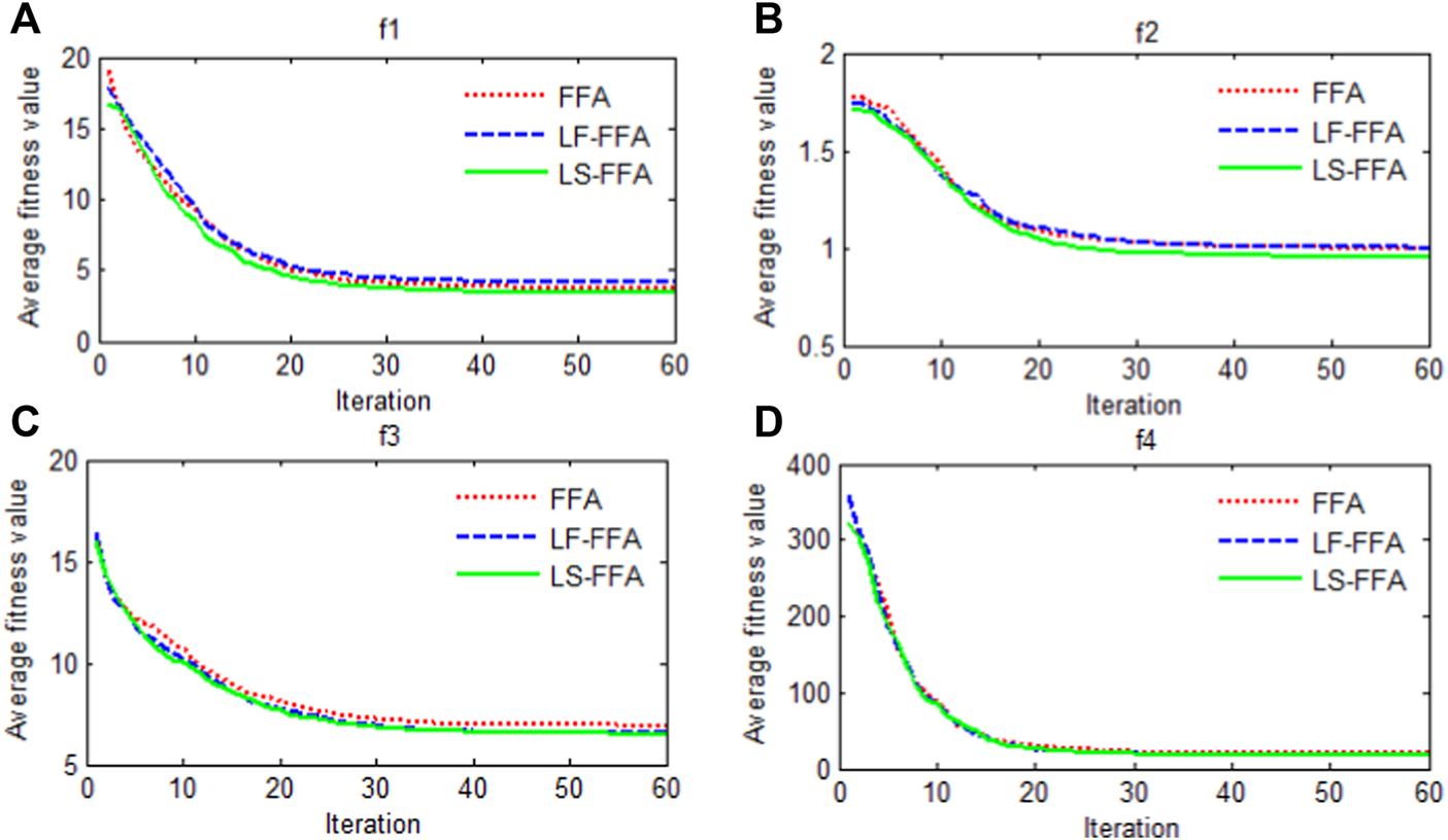
Trace of fitness for FA, LF-FA, and LS-FA.
FIGURE 6

Datasets of all five regions.
3.2 Data description
To verify the effectiveness of the proposed model, the datasets of electric load from 1 January 2018 to 1 February 2018 in NSW, QLD, SA, TAS, and VIC are used as the experimental data (Table 2 and Figure 6). The datasets of the electric load (MW) are retrieved from the website of energy security for all Australians (http://www.aemo.com.au/). The sample data used in this study are half-hourly electric load, and the total number of these five regions is 1,488. In this study, each dataset was divided into two sets: the training dataset including 960 data points (from 2018/1/1 0:30 to 2018/1/21 0:00) and the remaining as the test dataset (from 2018/1/21 0:30 to 2018/2/1 0:00).
TABLE 2
| Region | Training set | Test set | ||||||||
|---|---|---|---|---|---|---|---|---|---|---|
| NSW | QLD | SA | TAS | VIC | NSW | QLD | SA | TAS | VIC | |
| N | 960 | 960 | 960 | 960 | 960 | 528 | 528 | 528 | 528 | 528 |
| Mean | 8115.3 | 6720.3 | 1375.8 | 1102.9 | 4987.3 | 8818.6 | 6937.8 | 1503.0 | 1085.7 | 5578.9 |
| Std | 1350.0 | 873.1 | 417.8 | 70.3 | 1095.6 | 1493.2 | 905.8 | 357.5 | 86.3 | 1156.5 |
| Min | 5910.1 | 5258.4 | 653.2 | 950.8 | 3449.8 | 6197.6 | 5359.5 | 894.2 | 865.2 | 3683.1 |
| Max | 12230.6 | 8670.0 | 2879.9 | 1263.8 | 8999.2 | 12494.6 | 9020.4 | 2609.9 | 1256.5 | 9085.2 |
Statistical properties for each dataset.
3.3 Evaluation criteria
Because there is no confirmed universal standard method, this study adapts multiple error criteria to evaluate the effectiveness of the proposed hybrid model: the mean absolute error (MAE), root mean square error (RMSE), and mean absolute percent error (MAPE). The MAE, RMSE, and MAPE are applied to quantify the forecast error, and the performance of the model is reliable when their value is close to zero.
These three criteria are calculated as follows:where yi is the observed value, is the predicted value to yi, and N is the number of samples.
3.4 Selection of the kernel function
In this section, the selection of the kernel function in the SVR for electric load forecasting is discussed, and the data of five regions in Australia are applied to search for the fittest choice of the kernel function. First, four main kernel functions are provided when the model is established by SVR, and they are shown as follows:
Second, in order to find the best kernel function for forecasting electric load, we selected the last twelve half-hour load data (xn−12, xn−11, xn−10, …, xn−2, xn−1) as the input variables of SVR with different kernel functions, and the output variable is xn. At last, the best kernel function can be selected from the four kernel functions based on the performance of prediction. The experiment is performed, and the results of forecasting electric load based on different kernel functions are shown in Figure 7. It is obvious that the sigmoid kernel function has the worst performance, and the accuracy of the polynomial is just higher than it. In addition, the SVR based on the rbf kernel function and linear kernel function has better predictive results since it approaches the original data.
FIGURE 7

Predictive results of the SVR with different kernel functions.
In order to show the performances clearly, the three criteria (MAPE, MAE, and RMSE) of errors are calculated, and the results are shown in Table 3. The MAPE, MAE, and RMSE of the liner kernel function have the smallest values in all five regions. It must be noted that the rbf kernel function is just slightly poorer than the linear one. Moreover, it can be found that the polynomial and sigmoid functions are not suitable for electric load forecasting with larger errors. Based on this research, the linear is chosen as the kernel function of SVR in the study.
TABLE 3
| Criterion | Linear |
Polynomial |
rbf | Sigmoid | ||||||||
|---|---|---|---|---|---|---|---|---|---|---|---|---|
| MAPE | MAE | RMSE | MAPE | MAE | RMSE | MAPE | MAE | RMSE | MAPE | MAE | RMSE | |
| NSW | 1.13 | 99.08 | 123.22 | 8.58 | 786.68 | 964.58 | 1.38 | 122.32 | 155.59 | 61.88 | 5462.42 | 6533.04 |
| QLD | 1.04 | 73.10 | 91.57 | 4.41 | 312.24 | 401.27 | 1.27 | 88.97 | 113.14 | 38.79 | 2638.53 | 3916.17 |
| SA | 3.38 | 48.78 | 59.70 | 11.00 | 182.03 | 256.63 | 3.75 | 54.11 | 64.30 | 62.73 | 941.26 | 1154.82 |
| TAS | 1.38 | 14.85 | 20.99 | 5.04 | 51.30 | 99.96 | 1.70 | 17.78 | 25.19 | 24.34 | 242.74 | 612.28 |
| VIC | 2.07 | 112.63 | 137.15 | 9.28 | 565.44 | 763.20 | 2.28 | 124.07 | 151.53 | 91.87 | 5327.46 | 7083.36 |
Performance of the SVR with different kernel functions based on MAPE, MAE, and RMSE.
3.5 Process of LS-FA-SVR
In Section 2.5, the hybrid model LS-FA-SVR is established for short-term load forecasting. Here, the bandwidth of liner kernel and the regularization parameter of SVR can be optimized by the LS-FA. In this study, the numbers of fireflies, absorption coefficient, and iteration of LS-FA are 15, 1, and 20, respectively. Based on these, the prediction of short-term load in NSW, QLD, VIC, SA and TAS can be obtained.
3.6 Empirical analysis
To avoid some accidental situations which would cause unreliable conclusions, we conducted 30 runs for experiments in five regions, and three error indicators are recorded in Table 4 in each run.
TABLE 4
| Run No. | NSW | QLD | SA | TAS | VIC | ||||||||||
|---|---|---|---|---|---|---|---|---|---|---|---|---|---|---|---|
| MAPE | MAE | RMSE | MAPE | MAE | RMSE | MAPE | MAE | RMSE | MAPE | MAE | RMSE | MAPE | MAE | RMSE | |
| 1 | 0.866 | 91.237 | 112.178 | 0.819 | 59.613 | 75.405 | 2.777 | 42.653 | 51.459 | 1.116 | 11.390 | 10.356 | 1.363 | 89.422 | 109.661 |
| 2 | 0.933 | 91.397 | 112.035 | 0.753 | 59.866 | 75.402 | 2.689 | 42.857 | 51.378 | 1.131 | 11.338 | 10.424 | 1.346 | 89.354 | 109.649 |
| 3 | 1.048 | 91.211 | 112.124 | 0.582 | 59.756 | 75.571 | 2.832 | 42.701 | 51.371 | 1.138 | 11.487 | 10.402 | 1.438 | 89.289 | 109.463 |
| 4 | 0.892 | 91.307 | 112.078 | 0.673 | 59.861 | 75.288 | 2.718 | 42.624 | 51.360 | 1.043 | 11.440 | 10.318 | 1.243 | 89.362 | 109.710 |
| 5 | 0.804 | 91.467 | 112.038 | 0.793 | 59.838 | 75.523 | 2.716 | 42.704 | 51.385 | 1.048 | 11.424 | 10.430 | 1.281 | 89.365 | 109.837 |
| 6 | 0.951 | 91.380 | 112.071 | 0.699 | 59.726 | 75.462 | 2.693 | 42.554 | 51.402 | 1.061 | 11.424 | 10.408 | 1.367 | 89.426 | 109.517 |
| 7 | 0.830 | 91.363 | 112.133 | 0.666 | 59.853 | 75.420 | 2.767 | 42.724 | 51.458 | 1.218 | 11.381 | 10.263 | 1.390 | 89.280 | 109.722 |
| 8 | 0.905 | 91.442 | 112.044 | 0.652 | 59.831 | 75.308 | 2.811 | 42.737 | 51.387 | 1.069 | 11.567 | 10.371 | 1.294 | 89.279 | 109.558 |
| 9 | 0.905 | 91.460 | 112.077 | 0.686 | 59.718 | 75.474 | 2.652 | 42.752 | 51.291 | 1.086 | 11.256 | 10.444 | 1.364 | 89.299 | 109.648 |
| 10 | 0.965 | 91.416 | 112.118 | 0.824 | 59.745 | 75.365 | 2.754 | 42.686 | 51.469 | 1.092 | 11.335 | 10.389 | 1.404 | 89.321 | 109.570 |
| 11 | 1.031 | 91.331 | 112.079 | 0.682 | 59.636 | 75.429 | 2.732 | 42.728 | 51.281 | 1.202 | 11.441 | 10.276 | 1.394 | 89.307 | 109.647 |
| 12 | 0.970 | 91.253 | 111.879 | 0.784 | 59.727 | 75.369 | 2.791 | 42.647 | 51.452 | 1.108 | 11.323 | 10.468 | 1.347 | 89.454 | 109.552 |
| 13 | 0.880 | 91.348 | 112.161 | 0.807 | 59.755 | 75.398 | 2.809 | 42.859 | 51.469 | 1.103 | 11.356 | 10.441 | 1.270 | 89.373 | 109.685 |
| 14 | 1.026 | 91.370 | 112.218 | 0.889 | 59.602 | 75.275 | 2.683 | 42.542 | 51.369 | 1.069 | 11.422 | 10.424 | 1.254 | 89.289 | 109.686 |
| 15 | 0.921 | 91.213 | 112.109 | 0.757 | 59.721 | 75.470 | 2.775 | 42.685 | 51.394 | 1.133 | 11.367 | 10.317 | 1.297 | 89.364 | 109.664 |
| 16 | 0.950 | 91.286 | 112.156 | 0.732 | 59.819 | 75.410 | 2.756 | 42.695 | 51.324 | 1.022 | 11.325 | 10.544 | 1.293 | 89.429 | 109.651 |
| 17 | 1.101 | 91.397 | 112.010 | 0.715 | 59.825 | 75.440 | 2.938 | 42.698 | 51.274 | 1.132 | 11.329 | 10.405 | 1.395 | 89.379 | 109.647 |
| 18 | 0.936 | 91.311 | 112.100 | 0.517 | 59.785 | 75.496 | 2.653 | 42.580 | 51.448 | 0.975 | 11.268 | 10.464 | 1.257 | 89.454 | 109.520 |
| 19 | 0.903 | 91.342 | 112.152 | 0.778 | 59.769 | 75.399 | 2.711 | 42.740 | 51.367 | 1.130 | 11.489 | 10.221 | 1.453 | 89.303 | 109.728 |
| 20 | 1.076 | 91.205 | 112.122 | 1.018 | 59.737 | 75.456 | 2.783 | 42.803 | 51.485 | 1.020 | 11.367 | 10.428 | 1.304 | 89.557 | 109.658 |
| 21 | 0.987 | 91.256 | 112.003 | 0.805 | 59.738 | 75.469 | 2.690 | 42.774 | 51.253 | 1.221 | 11.470 | 10.410 | 1.216 | 89.322 | 109.643 |
| 22 | 1.049 | 91.240 | 112.212 | 0.962 | 59.714 | 75.455 | 2.704 | 42.565 | 51.516 | 1.152 | 11.361 | 10.410 | 1.291 | 89.237 | 109.392 |
| 23 | 0.948 | 91.286 | 112.062 | 0.673 | 59.609 | 75.375 | 2.770 | 42.617 | 51.434 | 1.074 | 11.394 | 10.287 | 1.248 | 89.387 | 109.560 |
| 24 | 0.965 | 91.481 | 112.172 | 0.824 | 59.943 | 75.511 | 2.789 | 42.858 | 51.326 | 1.041 | 11.563 | 10.437 | 1.306 | 89.391 | 109.602 |
| 25 | 0.929 | 91.292 | 112.064 | 0.666 | 59.749 | 75.371 | 2.872 | 42.721 | 51.480 | 1.085 | 11.395 | 10.502 | 1.426 | 89.357 | 109.758 |
| 26 | 0.990 | 91.352 | 112.283 | 0.864 | 59.827 | 75.449 | 2.714 | 42.693 | 51.544 | 0.934 | 11.351 | 10.386 | 1.321 | 89.211 | 109.665 |
| 27 | 1.010 | 91.248 | 112.087 | 0.644 | 59.884 | 75.447 | 2.737 | 42.628 | 51.406 | 1.231 | 11.424 | 10.429 | 1.213 | 89.367 | 109.685 |
| 28 | 0.841 | 91.413 | 112.305 | 0.616 | 59.589 | 75.411 | 2.818 | 42.695 | 51.385 | 1.097 | 11.317 | 10.269 | 1.436 | 89.377 | 109.528 |
| 29 | 1.038 | 91.219 | 112.098 | 0.800 | 59.687 | 75.389 | 2.759 | 42.858 | 51.435 | 1.064 | 11.384 | 10.379 | 1.414 | 89.331 | 109.560 |
| 30 | 0.971 | 91.315 | 112.171 | 0.818 | 59.841 | 75.469 | 2.808 | 42.854 | 51.305 | 1.068 | 11.266 | 10.475 | 1.311 | 89.330 | 109.485 |
| MEAN | 0.954 | 91.328 | 112.111 | 0.750 | 59.759 | 75.423 | 2.757 | 42.708 | 51.397 | 1.095 | 11.389 | 10.393 | 1.330 | 89.354 | 109.622 |
Performance of the LS-FA-SVR in NSW, QLD, SA, TAS, and VIC.
TABLE 5
| Region | DA-SVR | WOA-SVR | LS-FA-SVR | FA-SVR | ||||||||
|---|---|---|---|---|---|---|---|---|---|---|---|---|
| MAPE | MAE | RMSE | MAPE | MAE | RMSE | MAPE | MAE | RMSE | MAPE | MAE | RMSE | |
| NSW | 1.089 | 95.816 | 119.326 | 1.089 | 95.786 | 119.294 | 0.954 | 91.328 | 112.111 | 1.11 | 96.88 | 119.92 |
| QLD | 0.920 | 63.994 | 80.608 | 0.921 | 64.020 | 80.597 | 0.750 | 59.759 | 75.423 | 0.92 | 64.15 | 80.72 |
| SA | 3.379 | 48.791 | 59.686 | 3.376 | 48.763 | 59.656 | 2.757 | 42.708 | 51.397 | 3.41 | 49.12 | 60.13 |
| TAS | 1.376 | 20.961 | 14.797 | 1.376 | 14.796 | 20.964 | 1.095 | 11.389 | 10.393 | 1.38 | 13.93 | 14.49 |
| VIC | 1.702 | 116.478 | 94.186 | 1.701 | 94.169 | 116.498 | 1.330 | 89.354 | 109.622 | 1.70 | 94.26 | 116.60 |
Performance of the LS-FA-SVR based on MAE, MAPE, and RMSE compared to other models.
To verify the proposed model LS-FA-SVR, we conducted a forecasting experiment with the same electric load in NSW, QLD, SA; TAS and VIC. The comparisons of electric load values forecast using WOA-SVR, DA-SVR; FA-SVR, and the new proposed LS-FA-SVR are shown in Table 5 (Mirjalili and Lewis,2016; Mirjalili, 2016). It is clear that the new model LS-FA-SVR has the lowest MAE, MAPE, and RMSE, among all four models.
Comparing the LS-FA-SVR with FA-SVR, the difference between them is whether the logarithmic spiral has been improved. It can be found that after introducing the logarithmic spiral into the model, the MAE, MAPE, and RMSE in five regions all decrease, which indicates that the LS is necessary for forecasting the electric load. Moreover, this study compared LS-FA-SVR with two new optimizers which were developed in 2016. The two benchmark models are DA-SVR and WOA-SVR. Through the comparisons, the three error indicators have decreased significantly. For example, the RMSE of THE LS-FA-SVR in NSW is 112.111, yet the values of DA-SVR and WOA-SVR are 119.326 and 119.294, respectively. The smaller the values of MAE, MAPE, and RMSE, the better the model will be. According to the aforementioned results, it is clear that the proposed model LS-FA-SVR outperforms the three benchmark models for five regions, and they are shown in Figure 8.
FIGURE 8

Results of the SVR with different optimizers.
We applied the LS-FA-SVR model to the forecasting experiments for the five experimental datasets and stated the results in Table 5. As the last row of this table shows, the mean values of MAE, MAPE, and RMSE in NSW are 91.328, 0.954, and 112.111, respectively. Meanwhile, the mean values of MAE, MAPE, and RMSE in QLD are 59.759, 0.750, and 75.423, respectively. Moreover, Figure 8 clearly shows that the model LS-FA-SVR interprets the curves of the original electric load in NSW, QLD, SA, SAT, and VIC, which indicates that the new model gets a satisfactory performance and a high forecasting accuracy. Comprehensively considering the results of MAE, MAPE, and RMSE in NSW, QLD, SA, TAS, and VIC, it can be concluded that the LS-FA-SVR model is the best overall, and its prediction is the best.
4 Conclusion and future work
Accurate forecasting of the electric load can provide valuable references for economic managers and electric power system operators. The study proposed a hybrid model LS-FA-SVR for improving the forecasting accuracy, where the parameters of SVR are optimally determined by the optimization algorithm LS-FA. This hybrid approach can search over a wide range to expand the detection probability in the early period. It can increase the search efficiency in the late period. Hence, the LS-FA has a good performance to prevent the operation from falling into local optima and to ensure the convergence for searching the parameters of SVR. In addition, the empirical results show that the MAE, MAPE, and RMSE values of LS-FA-SVR are all modestly smaller than those of WOA-SVR, DA-SVR, and FA-SVR. Compared with these other methods, the new method has a strong ability to find the optimal solution, and the run time is shorter. In other words, LS-FA-SVR is an attractive and effective model which combines a novel optimization algorithm to determine the parameters of SVR. In future work, several research directions can be tried. More related variables can be taken into consideration. One possibility is to apply other factors which may influence electrical demand, such as the population and GDP, to obtain more comprehensive results (Li et al., 2017).
Statements
Data availability statement
The original contributions presented in the study are included in the article/Supplementary Material; further inquiries can be directed to the corresponding author.
Author contributions
WZ: formal analysis and writing—original draft; LG: writing—review and editing; YS: writing—review and editing; XL: writing—review and editing; and HZ: supervision, investigation, and project administration.
Conflict of interest
WZ and LG were employed by Nari Technology Co., Ltd, and YS was employed by State Grid Xiong’an Integrated Energy Service Co, Ltd. The remaining authors declare that the research was conducted in the absence of any commercial or financial relationships that could be construed as a potential conflict of interest.
Publisher’s note
All claims expressed in this article are solely those of the authors and do not necessarily represent those of their affiliated organizations, or those of the publisher, the editors, and the reviewers. Any product that may be evaluated in this article, or claim that may be made by its manufacturer, is not guaranteed or endorsed by the publisher.
References
1
Afrasiabi M. Mohammadi M. Rastegar M. Stankovic L. Afrasiabi S. Khazaei M. et al (2020). Deep-based conditional probability density function forecasting of residential loads. IEEE Trans. Smart Grid11, 3646–3657. 10.1109/tsg.2020.2972513
2
An N. Zhao W. Wang J. Shang D. Zhao E. (2013). Using multi-output feedforward neural network with empirical mode decomposition based signal filtering for electricity demand forecasting. Energy49, 279–288. 10.1016/j.energy.2012.10.035
3
Boser B. E. Guyon I. M. Vapnik V. N. (1992). A training algorithm for optimal margin classifiers. Proc. fifth Annu. workshop Comput. Learn. theory, 144–152.
4
Che J. Wang J. Tang Y. (2012). Optimal training subset in a support vector regression electric load forecasting model. Appl. Soft Comput.12, 1523–1531. 10.1016/j.asoc.2011.12.017
5
Chen B. Wang Y. (2021). Short-term electric load forecasting of integrated energy system considering nonlinear synergy between different loads. IEEE Access9, 43562–43573. 10.1109/access.2021.3066915
6
Chen Y. Xu P. Chu Y. Li W. Wu Y. Ni L. et al (2017). Short-term electrical load forecasting using the support vector regression (svr) model to calculate the demand response baseline for office buildings. Appl. Energy195, 659–670. 10.1016/j.apenergy.2017.03.034
7
Cui Z. Wu J. Ding Z. Duan Q. Lian W. Yang Y. et al (2021). A hybrid rolling grey framework for short time series modelling. Neural comput. Appl., 33, 11339–11353. 10.1007/s00521-020-05658-0
8
Feng C. Sun M. Zhang J. (2019). Reinforced deterministic and probabilistic load forecasting via q-learning dynamic model selection. IEEE Trans. Smart Grid11, 1377–1386. 10.1109/tsg.2019.2937338
9
Hong W.-C. (2011). Electric load forecasting by seasonal recurrent svr (support vector regression) with chaotic artificial bee colony algorithm. Energy36, 5568–5578. 10.1016/j.energy.2011.07.015
10
Kaur A. Nonnenmacher L. Coimbra C. F. (2016). Net load forecasting for high renewable energy penetration grids. Energy114, 1073–1084. 10.1016/j.energy.2016.08.067
11
Kaveh A. Khayatazad M. (2012). A new meta-heuristic method: Ray optimization. Comput. Struct.112, 283–294. 10.1016/j.compstruc.2012.09.003
12
Kavousi-Fard A. Samet H. Marzbani F. (2014). A new hybrid modified firefly algorithm and support vector regression model for accurate short term load forecasting. Expert Syst. Appl.41, 6047–6056. 10.1016/j.eswa.2014.03.053
13
Kisi O. Shiri J. Karimi S. Shamshirband S. Motamedi S. Petković D. et al (2015). A survey of water level fluctuation predicting in urmia lake using support vector machine with firefly algorithm. Appl. Math. Comput.270, 731–743. 10.1016/j.amc.2015.08.085
14
Kong W. Dong Z. Y. Hill D. J. Luo F. Xu Y. (2017). Short-term residential load forecasting based on resident behaviour learning. IEEE Trans. Power Syst.33, 1087–1088. 10.1109/tpwrs.2017.2688178
15
Li W. Kong D. Wu J. (2017). A new hybrid model fpa-svm considering cointegration for particular matter concentration forecasting: A case study of kunming and yuxi, China. Comput. Intell. Neurosci.2017, 2843651. 10.1155/2017/2843651
16
Mirjalili S. (2016). Dragonfly algorithm: A new meta-heuristic optimization technique for solving single-objective, discrete, and multi-objective problems. Neural comput. Appl.27, 1053–1073. 10.1007/s00521-015-1920-1
17
Mirjalili S. Lewis A. (2016). The whale optimization algorithm. Adv. Eng. Softw.95, 51–67. 10.1016/j.advengsoft.2016.01.008
18
Mirjalili S. Mirjalili S. M. Lewis A. (2014). Grey wolf optimizer. Adv. Eng. Softw.69, 46–61. 10.1016/j.advengsoft.2013.12.007
19
Najafzadeh M. Etemad-Shahidi A. Lim S. Y. (2016). Scour prediction in long contractions using anfis and svm. Ocean. Eng.111, 128–135. 10.1016/j.oceaneng.2015.10.053
20
Najafzadeh M. Saberi-Movahed F. Sarkamaryan S. (2018). Nf-gmdh-based self-organized systems to predict bridge pier scour depth under debris flow effects. Mar. Georesources Geotechnol.36, 589–602. 10.1080/1064119x.2017.1355944
21
Olorunda O. Engelbrecht A. P. (2008). “Measuring exploration/exploitation in particle swarms using swarm diversity,” in 2008 IEEE congress on evolutionary computation (IEEE world congress on computational intelligence), Hong Kong, China, 01-06 June 2008 (IEEE), 1128–1134.
22
Peng L.-L. Fan G.-F. Huang M.-L. Hong W.-C. (2016). Hybridizing demd and quantum pso with svr in electric load forecasting. Energies9, 221. 10.3390/en9030221
23
Stojanović M. Božić M. Stajić Z. Milošević M. (2013). Ls-svm model for electrical load prediction based on incremental training set update. Przeglad Elektrotechniczny89, 194–198.
24
Vapnik V. (1999). The nature of statistical learning theory. Berlin/Heidelberg, Germany: Springer science & business media.
25
Walster G. Hansen E. Sengupta S. (1985). Test results for a global optimization algorithm. Numer. Optim.1984, 272–287.
26
Wang C. Hou Y. Gao Q. Hou R. Deng T. (2016). Electric load simulator system control based on adaptive particle swarm optimization wavelet neural network with double sliding modes. Adv. Mech. Eng.8, 168781401666426. 10.1177/1687814016664261
27
Wang D. Liu L. Jia H. Wang W. Zhi Y. Meng Z. et al (2018). Review of key problems related to integrated energy distribution systems. CSEE J. Power Energy Syst.4, 130–145. 10.17775/cseejpes.2018.00570
28
Wu J. Wang Y.-G. Tian Y.-C. Burrage K. Cao T. (2021). Support vector regression with asymmetric loss for optimal electric load forecasting. Energy223, 119969. 10.1016/j.energy.2021.119969
29
Xiao L. Shao W. Yu M. Ma J. Jin C. (2017). Research and application of a combined model based on multi-objective optimization for electrical load forecasting. Energy119, 1057–1074. 10.1016/j.energy.2016.11.035
30
Yan G. Tang G.-h. Xiong J.-m. (2012). “Electric load forecasting based on improved ls-svm algorithm,” in Proceedings of the 10th World Congress on Intelligent Control and Automation, Beijing, China, 06-08 July 2012 (IEEE), 3064–3067.
31
Yang X.-S. Deb S. (2009). “Cuckoo search via lévy flights,” in 2009 World congress on nature & biologically inspired computing (NaBIC), Coimbatore, India, 09-11 December 2009 (IEEE), 210–214.
32
Yang X.-S. (2010a). “Firefly algorithm, levy flights and global optimization,” in Research and development in intelligent systems XXVI (New York, United States: Springer), 209–218.
33
Yang X.-S. (2010b). Firefly algorithm, stochastic test functions and design optimisation. Int. J. Bio-inspired Comput.2, 78. 10.1504/ijbic.2010.032124
34
Yang X.-S. (2009). “Firefly algorithms for multimodal optimization,” in International symposium on stochastic algorithms (New York, United States: Springer), 169–178.
35
Yang Y. Liu Q. Yue D. Han Q.-L. (2021a). Predictor-based neural dynamic surface control for bipartite tracking of a class of nonlinear multiagent systems. IEEE Trans. Neural Netw. Learn. Syst.33, 1791–1802. 10.1109/tnnls.2020.3045026
36
Yang Y. Tao Z. Qian C. Gao Y. Zhou H. Ding Z. et al (2021b). A hybrid robust system considering outliers for electric load series forecasting. Appl. Intell. (Dordr).1–23, 1630–1652. 10.1007/s10489-021-02473-5
37
Yang Y. Wang Z. Gao Y. Wu J. Zhao S. Ding Z. et al (2022a). An effective dimensionality reduction approach for short-term load forecasting. Electr. Power Syst. Res.210, 108150. 10.1016/j.epsr.2022.108150
38
Yang Y. Zhou H. Gao Y. Wu J. Wang Y.-G. Fu L. et al (2022b). Robust penalized extreme learning machine regression with applications in wind speed forecasting. Neural comput. Appl.34, 391–407. 10.1007/s00521-021-06370-3
39
Yang Y. Zhou H. Wu J. Ding Z. Wang Y.-G. (2022c). Robustified extreme learning machine regression with applications in outlier-blended wind-speed forecasting. Appl. Soft Comput.122, 108814. 10.1016/j.asoc.2022.108814
40
Yang Y. Zhou H. Wu J. Liu C.-J. Wang Y.-G. (2022d). A novel decompose-cluster-feedback algorithm for load forecasting with hierarchical structure. Int. J. Electr. Power & Energy Syst.142, 108249. 10.1016/j.ijepes.2022.108249
41
Zhang G. Guo J. (2019). A novel method for hourly electricity demand forecasting. IEEE Trans. Power Syst.35, 1351–1363. 10.1109/tpwrs.2019.2941277
42
Zhang S. Wu J. Jia Y. Wang Y.-G. Zhang Y. Duan Q. et al (2021). A temporal lasso regression model for the emergency forecasting of the suspended sediment concentrations in coastal oceans: Accuracy and interpretability. Eng. Appl. Artif. Intell.100, 104206. 10.1016/j.engappai.2021.104206
43
Zhang S. Wu J. Wang Y.-G. Jeng D.-S. Li G. (2022a). A physics-informed statistical learning framework for forecasting local suspended sediment concentrations in marine environment. Water Res.218, 118518. 10.1016/j.watres.2022.118518
44
Zhang Y. Wu J. Zhang S. Li G. Jeng D.-S. Xu J. et al (2022b). An optimal statistical regression model for predicting wave-induced equilibrium scour depth in sandy and silty seabeds beneath pipelines. Ocean. Eng.258, 111709. 10.1016/j.oceaneng.2022.111709
Summary
Keywords
electric load, time series forecasting, firefly algorithm, support vector regression, logarithmic spiral, management of power system
Citation
Zhang W, Gu L, Shi Y, Luo X and Zhou H (2022) A hybrid SVR with the firefly algorithm enhanced by a logarithmic spiral for electric load forecasting. Front. Energy Res. 10:977854. doi: 10.3389/fenrg.2022.977854
Received
25 June 2022
Accepted
11 July 2022
Published
02 September 2022
Volume
10 - 2022
Edited by
Qihe Shan, Dalian Maritime University, China
Reviewed by
Jinran Wu, Queensland University of Technology, Australia
Zhesen Cui, Changzhi University, China
Shaotong Zhang, Ocean University of China, China
Updates
Copyright
© 2022 Zhang, Gu, Shi, Luo and Zhou.
This is an open-access article distributed under the terms of the Creative Commons Attribution License (CC BY). The use, distribution or reproduction in other forums is permitted, provided the original author(s) and the copyright owner(s) are credited and that the original publication in this journal is cited, in accordance with accepted academic practice. No use, distribution or reproduction is permitted which does not comply with these terms.
*Correspondence: Weiguo Zhang, 230209330@seu.edu.cn
This article was submitted to Smart Grids, a section of the journal Frontiers in Energy Research
Disclaimer
All claims expressed in this article are solely those of the authors and do not necessarily represent those of their affiliated organizations, or those of the publisher, the editors and the reviewers. Any product that may be evaluated in this article or claim that may be made by its manufacturer is not guaranteed or endorsed by the publisher.