Adaptive individual residential load forecasting based on deep learning and dynamic mirror descent

1 Introduction

As advanced metering infrastructure (AMI) is being widely deployed in the modern power system, especially, smart meters, a growing number of granular data of residential electricity consumption has become easily available on a large scale (Sajjad et al., 2016; Xie et al., 2018). This huge amount of data enables power network operators to motivate residential customers to actively participate in demand side management (DSM) through a wide range of various demand response programs (DRPs), for example, time-of-use pricing (Zhou et al., 2016; Ponocko and Milanovic, 2018). As part of DSM, residential load forecasting is a significantly important but challenging task for power network operators, due to great irregularity and uncertainty of residential load (Welikala et al., 2019). As a result, addressing the challenges of residential load forecasting plays a crucial role in interactions between network operators and residential customers, efficient and cost-effective grid operations, and household energy consumption optimizations.

At present, residential load forecasting is generally categorized into two classes - aggregate and individual. More specifically, data analytics for aggregate residential load forecasting mainly include support vector regression (SVR) (Humeau et al., 2013; Wijaya et al., 2015), random forest (Goehry et al., 2020), artificial neural networks (ANNs) (Marinescu et al., 2013; Marinescu et al., 2014; Quilumba et al., 2015; Campos and Silva, 2016; Stephen et al., 2017; Wang et al., 2018; Oprea and Bara, 2019), and deep neural networks (DNNs) (Zheng et al., 2018; Zou et al., 2019). Besides, these methods tend to be combined with clustering techniques, for instance, k-means clustering, in order to improve the forecasting performance. In general, a number of models based on these methods have obtained a desirable level of prediction accuracy on aggregate residential load forecasting. This is because a variety of behaviours of residential customers can smoothen out their overall load profile at the aggregate level, therefore generating an easily identifiable energy consumption pattern.

However, compared to aggregate residential load forecasting, only a few researchers have attempted to explore individual residential load forecasting so far. Some traditional machine learning methods, for instance, ANNs, are still applied to forecast individual residential load (Paterakis et al., 2016; Xu et al., 2016; Vossen et al., 2018; Dinesh et al., 2019; Wu et al., 2020). During recent years, DNNs, such as recurrent neural networks (RNNs) and long short-term memory (LSTM) networks (Gan et al., 2017; Kong et al., 2017; Hossen et al., 2018; Shi et al., 2018; Kong et al., 2019; Alhussein et al., 2020; Wang et al., 2020; Lin et al., 2021), have been largely adopted due to their superior capability in extracting complex patterns. Although existing DNN models have mostly achieved a comparatively higher prediction accuracy than many traditional machine learning models, they are essentially trained on a limited amount of residential load data offline and then applied to perform forecasting online. As a result, these well-trained offline models are likely to encounter many sudden changes of residential load when forecasting online, which are not included in training. This is because individual residential load can be extremely volatile and uncertain, which would have a significantly negative effect on the forecasting performance of the DNN models.

To address the issue of volatility of individual residential load in forecasting, this paper presents a method for short-term individual residential load forecasting, which is able to adjust the forecasting error dynamically. Specifically, the key contributions of the paper are summarized as follows:

1) Firstly, it presents an LSTM based deep learning method empowered with dynamic mirror descent (DMD) for adaptive individual residential load forecasting.

2) Secondly, it modifies the original DMD to make it feasible for adjusting residential load forecasting.

3) Thirdly, it devises a comprehensive feature expression strategy to describe load characteristics at each time step in order to form the input of the forecasting model.

4) Finally, the proposed method is validated and compared with a published benchmark method on a real-life Irish residential load dataset, and the influence of the modified DMD on the forecasting performance of the proposed method is investigated in detail.

The remainder of this paper is organized as follows. Section 2 reports a comprehensive literature review on residential load forecasting. Section 3 briefly introduces recurrent neural networks and LSTM networks, and then details the modifications made on the original DMD. Section 4 integrates DMD into an LSTM based deep learning method for adaptive individual residential load forecasting. In Section 5, the proposed residential load forecasting method is evaluated on a real-life Irish residential load dataset. Finally, Section 6 concludes the paper and points out some future work.

2 Review on residential load forecasting

A number of research works have been presented in the area of aggregate residential load forecasting. Wijaya et al. (2015) designed a short-term cluster-based aggregate residential load forecasting strategy. It firstly clusters residential customers, then forecasts the energy consumption of each cluster separately through SVR, and finally aggregates the energy consumption forecasts of all clusters. Similar to Wijaya et al. (2015), Humeau et al. (2013) developed a residential load forecasting method for the district level, which combines k-means clustering with SVR. Different from Wijaya et al. (2015) and Humeau et al. (2013), Goehry et al. (2020) employed hierarchical clustering and random clustering respectively to divide residential customers into subsets and applied random forests to build the forecasting model for each subset.

ANNs have also been commonly applied to forecast residential load at the aggregate level. For example, a dynamic forecasting mechanism was proposed to monitor small-scale residential electricity demand and detect anomalous pattern changes in Marinescu et al. (2014). A self-organizing map is employed for anomalous day detection, and an ANN prediction model changes its input neurons according to a previously detected and recorded match in a database of anomalous days in order to conduct demand prediction for anomalous days. Wang et al. (2018) proposed an ensemble method for short-term aggregate residential load forecasting, which produces the forecasts for all load subprofiles based on hierarchical clustering and ANNs, and then combines all the forecasts with different weights to obtain the final forecasting result of the aggregate residential load. Quilumba et al. (2015) presented a three-step aggregate residential load forecasting approach, based on k-means clustering and ANNs. In Marinescu et al. (2013) and Campos and Silva (2016), a comprehensive performance comparison was made between ANNs and some other prediction models, such as auto-regression and auto-regressive integrated moving average. Moreover, a gated recurrent unit (GRU) neural network based approach was developed to perform short-term load forecasting for residential community (Zheng et al., 2018). Also, it uses least absolute shrinkage and selection operator (LASSO) and partial correlation analysis to explore the influences of temperature, humidity, rainfall, and wind speed on residential load in order to determine the input variables for the forecasting model.

In summary, aggregate residential load is comparatively easier to forecast than individual residential load, because individual behaviors have the features of volatility and uncertainty in energy consumption. As a result, existing forecasting models on aggregate residential load have obtained a satisfactory level of prediction accuracy.

By contrast, only a few efforts have been made towards individual residential load forecasting. Xu et al. (2016) proposed a k-nearest vector auto-regressive framework with exogenous input to spatial-temporally model household electricity demand. Dinesh et al. (2019) presented a forecasting approach to the power consumption of a single household, which is based on non-intrusive load monitoring (NILM) and graph spectral clustering. Different from Xu et al. (2016) and Dinesh et al. (2019), Vossen et al. (2018) developed a probabilistic forecasting model to describe the uncertainty of individual residential load using two different types of density-estimation ANNs respectively. In Wu et al. (2020), a boosting-based framework for multiple kernel learning regression was presented to forecast individual residential load. It not only adopts boosting to learn an ensemble of multiple kernel regressors, but also applies transfer learning to forecast the load of the residential customer which has a very limited amount of energy consumption data. In addition, Gan et al. (2017) employed a quantile LSTM network to perform probabilistic residential load forecasting at the individual level. In Alhussein et al. (2020), a hybrid model combining a convolutional neural network and an LSTM network was proposed to forecast the individual household load. Wang et al. (2020) designed a framework for short-term individual residential load forecasting. It firstly partitions historical load data by clustering to train multiple LSTM models, and then uses a fully connected cascade neural network to fuse the multiple LSTM models. Shi et al. (2018) proposed a novel pooling-based deep RNN to avoid overfitting during residential load forecasting. It batches the load profiles of a group of residential customers into an input pool in order to increase data diversity and volume. Also, Lin et al. (2021) presented a graph neural network based method for individual residential load forecasting, which aims to capture both temporal information of historical load and spatial information of neighbouring households in order to improve the forecasting accuracy. In Hossen et al. (2018), different types of DNNs, such as RNNs and LSTM networks, were applied to short-term individual residential load forecasting and a performance comparison was conducted among them. Furthermore, automatic hyperparameter tuning was utilised to select an optimal hyperparameter combination for an LSTM network in order to improve the accuracy of individual residential load forecasting (Kong et al., 2017).

Although a variety of forecasting models for individual residential load have been developed, their training data is unable to include all the cases on residential energy consumption, as individual residential load tends to change dramatically over time, which leads to a poor prediction accuracy when they are applied online.

3 Methodology

3.1 Long short term memory model

As a sequence based model, RNNs are capable of establishing excellent temporal correlation between previous and current information (Chen et al., 2016; Tolosana et al., 2018). This characteristic makes RNNs an ideal candidate for short-term residential load forecasting, because the residential load consumption pattern has a strong and complex relationship between adjacent time steps (Kong et al., 2019). However, in terms of the specific implementation, a special RNN, called the LSTM network, is employed in this paper, as it significantly improves the performance of the general RNN. In this section, the RNN architecture is firstly introduced, and then the LSTM unit is explained.

3.1.1 Recurrent neural networks

In the working process, the RNN aims to map the input sequence of x values into corresponding sequential outputs: y. Specifically, the learning process conducts every single time step from $\mathit{t}=1$ to $\mathit{t}=\tau$. For time step t, the network neuron parameters at the ${\mathit{l}}^{\text{th}}$ layer update their shared states with the following equations (Shi et al., 2018):

${\mathit{a}}_1^{\left(\mathit{t}\right)}={\mathit{b}}_1+{\mathit{W}}_1\cdot {\mathit{h}}_1^{\left(\mathit{t}-1\right)}+{\mathit{U}}_1\cdot {\mathit{x}}^{\left(\mathit{t}\right)}(1)$

${\mathit{h}}_{\mathit{l}}^{\left(\mathit{t}\right)}={\mathit{f}}_{\text{activation}}\left({\mathit{a}}_{\mathit{l}}^{\left(\mathit{t}\right)}\right)\left(\mathit{l}=1,2,\cdots ,\mathit{N}\right)(2)$

${\mathit{a}}_{\mathit{l}}^{\left(\mathit{t}\right)}={\mathit{b}}_{\mathit{l}}+{\mathit{W}}_{\mathit{l}}\cdot {\mathit{h}}_{\mathit{l}}^{\left(\mathit{t}-1\right)}+{\mathit{U}}_{\mathit{l}}\cdot {\mathit{h}}_{\mathit{l}-1}^{\left(\mathit{t}\right)}\left(\mathit{l}=2,3,\cdots ,\mathit{N}\right)(3)$

${\mathit{y}}^{\left(\mathit{t}\right)}={\mathit{b}}_{\mathit{N}}+{\mathit{W}}_{\mathit{N}}\cdot {\mathit{h}}_{\mathit{N}}^{\left(\mathit{t}-1\right)}+{\mathit{U}}_{\mathit{N}}\cdot {\mathit{h}}_{\mathit{N}}^{\left(\mathit{t}\right)}(4)$

$L=f_{\mathrm{loss}}\left(y^{\left(t\right)},y_{\mathrm{target}}^{\left(t\right)}\right)(5)$

where ${\mathit{x}}^{\left(\mathit{t}\right)}$ is the data input at time step t, ${\mathit{y}}^{\left(\mathit{t}\right)}$ is the corresponding forecast, ${\mathit{y}}_{\text{target}}^{\left(\mathit{t}\right)}$ is the true output at time step t, ${\mathit{h}}_{\mathit{l}}^{\left(\mathit{t}\right)}$ is the shared states of the ${\mathit{l}}^{\text{th}}$ layer at time step t, N is the total layer number of the network, and ${\mathit{a}}_{\mathit{l}}^{\left(\mathit{t}\right)}$ is the input of the ${\mathit{l}}^{\text{th}}$ layer at time step t, which consists of three components: 1) the input ${\mathit{x}}^{\left(\mathit{t}\right)}$ at time step t or the shared states ${\mathit{h}}_{\mathit{l}-1}^{\left(\mathit{t}\right)}$ of the ${\mathit{l}-1}^{\text{th}}$ layer at time step t; 2) the bias ${\mathit{b}}_{\mathit{l}}$ of the ${\mathit{l}}^{\text{th}}$ layer; 3) the shared states ${\mathit{h}}_{\mathit{l}}^{\left(\mathit{t}-1\right)}$ of the ${\mathit{l}}^{\text{th}}$ layer at time step t-1.

Due to their shared states, RNNs are able to learn dependency contained in the previous time steps.

3.1.2 LSTM units

RNNs are trained by backpropagation through time, but learning long-term dependency with RNNs is difficult because of gradient vanishing or exploding (Kong et al., 2019). In order to overcome these two issues, an LSTM unit is introduced, and LSTM has gradually become the most popular structure of RNNs in solving many time series problems.

Let $\left\{{\mathit{x}}_1{,\mathit{x}}_2,\cdots ,{\mathit{x}}_{\mathit{T}}\right\}$ denote a typical input sequence for an LSTM unit, where ${\mathit{x}}_{\mathit{t}}\in {\mathit{R}}^{\mathit{k}}$ represents a k-dimensional vector of real values at time step t. In order to establish temporal relations, the LSTM unit defines and maintains an internal memory cell state throughout the life cycle, which is the most important element of the LSTM unit. The memory cell state ${\mathit{s}}_{\mathit{t}-1}$ interacts with the intermediate output ${\mathit{h}}_{\mathit{t}-1}$ and the subsequent input ${\mathit{x}}_{\mathit{t}}$ to determine which elements of the internal state vector should be updated, maintained, or erased according to the outputs of the previous time step and the inputs of the present time step. Apart from the internal state, the LSTM unit also defines the input node ${\mathit{g}}_{\mathit{t}}$, the input gate ${\mathit{i}}_{\mathit{t}}$, the forget gate ${\mathit{f}}_{\mathit{t}}$, and the output gate ${\mathit{o}}_{\mathit{t}}$. The formulations of all nodes in the LSTM unit are presented below from (6) to (11) (Kong et al., 2019):

${\mathit{f}}_{\mathit{t}}=\mathit{\sigma }\left({\mathit{W}}_{\mathit{fx}}{\mathit{x}}_{\mathit{t}}+{\mathit{W}}_{\mathit{fh}}{\mathit{h}}_{\mathit{t}-1}+{\mathit{b}}_{\mathit{f}}\right)(6)$

${\mathit{i}}_t=\mathit{\sigma }\left({\mathit{W}}_{ix}{\mathit{x}}_t+{\mathit{W}}_{ih}{\mathit{h}}_{t-1}+{\mathit{b}}_i\right)(7)$

${\mathit{g}}_{\mathit{t}}=\mathit{\Phi }\left({\mathit{W}}_{\mathit{gx}}{\mathit{x}}_{\mathit{t}}+{\mathit{W}}_{\mathit{gh}}{\mathit{h}}_{\mathit{t}-1}+{\mathit{b}}_{\mathit{g}}\right)(8)$

${\mathit{o}}_t=\sigma \left({\mathit{W}}_{ox}{\mathit{x}}_t+{\mathit{W}}_{oh}{\mathit{h}}_{t-1}+{\mathit{b}}_o\right)(9)$

${\mathit{s}}_t={\mathit{g}}_t\odot i_t+{\mathit{s}}_{t-1}\odot {\mathit{f}}_t(10)$

${\mathit{h}}_t=\mathit{\Phi }\left({\mathit{s}}_t\right)\odot o_t(11)$

where ${\mathit{W}}_{\mathit{fx}}$, ${\mathit{W}}_{\mathit{fh}}$, ${\mathit{W}}_{\mathit{ix}}$, ${\mathit{W}}_{\mathit{ih}}$, ${\mathit{W}}_{\mathit{gx}}$, ${\mathit{W}}_{\mathit{gh}}$, ${\mathit{W}}_{\mathit{ox}}$, and ${\mathit{W}}_{\mathit{oh}}$ denote the weight matrices of the corresponding inputs of the network activation functions, $\odot$ denotes the element-wise multiplication, $\sigma$ denotes the sigmoid activation function, and $\mathrm{\Phi }$ denotes the tanh activation function.

In each time step, the memory cell state has three operations: 1) discard useless information from the memory cell state ${\mathit{s}}_{\mathit{t}}$; 2) add the new information ${\mathit{i}}_{\mathit{t}}$ extracted from the input ${\mathit{x}}_{\mathit{t}}$ and the intermediate output ${\mathit{h}}_{\mathit{t}-1}$ into the memory cell state ${\mathit{s}}_{\mathit{t}}$; 3) determine the new intermediate output ${\mathit{h}}_{\mathit{t}}$ from the memory cell state ${\mathit{s}}_{\mathit{t}}$. Thus, the memory cell state is capable to keep useful information for a long time and result in RNN performance enhancement.

3.2 Dynamic mirror descent

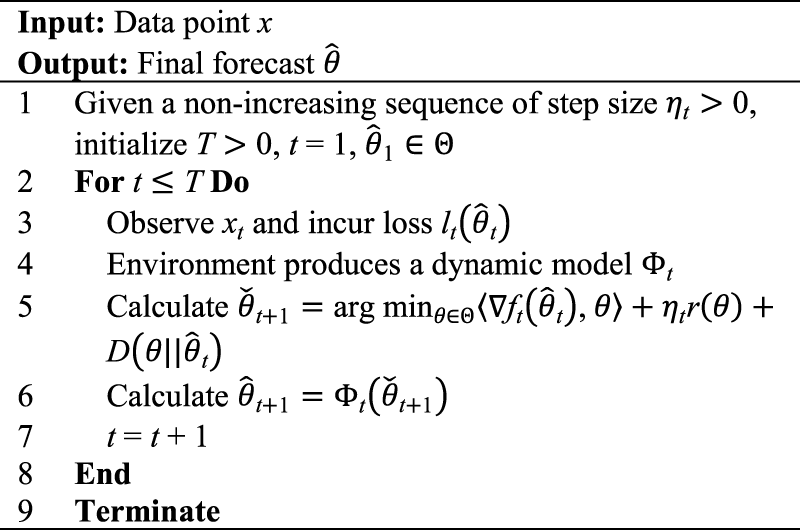
As an online learning method, dynamic mirror descent (DMD) is capable to incorporate a dynamic model in the learning process, and effectively minimize the loss and estimate time-varying system states (Hall and Willett, 2015; Ledva et al., 2015). DMD is executed by two main steps: 1) an observation-based update incorporates the new measurement into the parameter prediction; 2) a model-based update advances the parameter prediction to the next time step. The frequently used notations in DMD are given in Table 1, and the detailed steps of DMD are presented in Algorithm 1.

TABLE 1

TABLE 1. Frequently used notations in dynamic mirror descent.

Algorithm 1. Dynamic Mirror Descent

In order to apply DMD to adjust the forecasted value of residential load dynamically, following the work presented in Ledva et al. (2018), a few modifications are made to the original DMD. The idea is that the concept of the original DMD is still adopted but it is not a direct implementation of the original DMD. In other words, the modified DMD considers the forecasting model as a black box and simply adjusts its output with the measured and forecasted values. Hence, the modified DMD is formulated as follows:

${\widehat{k}}_{t+1}=\mathrm{a}\mathrm{r}\mathrm{g}{\min }_{\theta \in \Theta }\eta \langle \nabla l_t\left({\widehat{\theta }}_t\right),\theta \rangle +D\left(\theta ||{\widehat{k}}_t\right)(12)$

${\stackrel{\mathrm{ˇ}}{\theta }}_{t+1}=\mathrm{\Phi }\left({\overline{\theta }}_t\right)(13)$

${\widehat{\theta }}_{t+1}={\stackrel{\mathrm{ˇ}}{\theta }}_{t+1}+{\widehat{k}}_{t+1}(14)$

where $\nabla {\mathit{l}}_{\mathit{t}}$ is an arbitrary sub-gradient function of $l_t\left(\cdot \right)$; ${\widehat{k}}_t$ is the adjustment variable accumulating the deviation between the forecasted and measured values; $\eta$ is the constant step size; $\mathrm{\Phi }$ is the residential load forecasting model; ${\overline{\theta }}_{\mathit{t}}$ is the input data of $\mathrm{\Phi }$. The model-based update (13) only computes an intermediate prediction ${\stackrel{\mathrm{ˇ}}{\theta }}_{\mathit{t}+1}$ without the real measurement influencing ${\stackrel{\mathrm{ˇ}}{\theta }}_{\mathit{t}+1}$. The measurement-based update and the model-based prediction are combined in (14) to obtain a final prediction ${\widehat{\theta }}_{\mathit{t}+1}$.

In this paper, for simplicity, the loss function ${\mathit{l}}_{\mathit{t}}\left({\widehat{\theta }}_{\mathit{t}}\right)$ is selected as ${\mathit{l}}_{\mathit{t}}\left({\widehat{\theta }}_{\mathit{t}}\right)=\frac{1}{2}\mathrm{\Vert }{\widehat{\theta }}_{\mathit{t}}-{\mathit{y}}_t{\mathrm{\Vert }}_2^2$, while the Bregman divergence $D\left(\theta \mathrm{\Vert }{\widehat{k}}_t\right)$ is selected as. $D\left(\theta \mathrm{\Vert }{\widehat{k}}_t\right)=\frac{1}{2}\mathrm{\Vert }\theta -{\widehat{k}}_t{\mathrm{\Vert }}_2^2$ Thus, the convex function (12) can be simplified as the following:

${\widehat{k}}_{t+1}={\widehat{k}}_t+\eta \left(y_t-{\widehat{\theta }}_t\right)(15)$

where ${\mathit{y}}_{\mathit{t}}$ and ${\widehat{\theta }}_{\mathit{t}}$ are the real measurement and the final forecast of residential load respectively. As a result, the modified DMD is formed using (13–15).

4 Adaptive individual residential load forecasting

4.1 Implementation process

Due to high volatility and uncertainty of individual residential load, a comprehensive feature expression strategy is devised in order to describe the details of the energy consumption at each time step. So, the input features of a data sample ${\mathit{S}}_{\mathit{t}}$ at a particular time step t are detailed as follows:

1) the sequence of the residential load for the past T time steps ${\mathbf{E}}_{\mathit{t}}\in {\mathbf{R}}^{\mathit{T}}$ is formed as:

${\mathbf{E}}_{\mathit{t}}=\left[{\mathit{e}}_{\mathit{t}-\mathit{T}},\cdots ,{\mathit{e}}_{\mathit{t}-2},{\mathit{e}}_{\mathit{t}-1}\right](16)$

where ${\mathit{e}}_{\mathit{t}}$ is the energy consumption (kWh) at time step t;

2) the sequence of the half-hourly indexes for the past T time steps ${\mathbf{D}}_{\mathit{t}}\in {\mathbf{R}}^{\mathit{T}}$ is formed as:

${\mathbf{D}}_{\mathit{t}}=\left[{\mathit{d}}_{\mathit{t}-\mathit{T}},\cdots ,{\mathit{d}}_{\mathit{t}-2},{\mathit{d}}_{\mathit{t}-1}\right](17)$

where ${\mathit{d}}_{\mathit{t}}\in \left[1,48\right]$ is the half-hourly index for time step t, because the sampling frequency is once every half an hour;

3) the sequence of the day indexes for the past T time steps ${\mathbf{W}}_{\mathit{t}}\in {\mathbf{R}}^{\mathit{T}}$ is formed as:

${\mathbf{W}}_{\mathit{t}}=\left[{\mathit{w}}_{\mathit{t}-\mathit{T}},\cdots ,{\mathit{w}}_{\mathit{t}-2},{\mathit{w}}_{\mathit{t}-1}\right](18)$

where ${\mathit{w}}_{\mathit{t}}\in \left[1,7\right]$ is the day index for time step t, as there are 7 days in a week;

4) the sequence of the holiday signs for the past T time steps ${\mathbf{H}}_{\mathit{t}}\in {\mathbf{R}}^{\mathit{T}}$ is formed as:

${\mathbf{H}}_{\mathit{t}}=\left[{\mathit{h}}_{\mathit{t}-\mathit{T}},\cdots ,{\mathit{h}}_{\mathit{t}-2},{\mathit{h}}_{\mathit{t}-1}\right](19)$

where ${\mathit{h}}_{\mathit{t}}$ is the holiday sign for time step t, which is either one or 2, and one denotes non-holiday and two denotes holiday (in this paper, it is assumed that weekdays are non-holiday and weekends are holiday).

Thus, a data sample ${\mathit{S}}_{\mathit{t}}$ is a matrix of a concatenation of the four sequences, expressed below:

${\mathbf{S}}_{\mathit{t}}=\left[{\mathbf{E}}_{\mathit{t}}^{\mathbf{T}},{\mathit{D}}_{\mathit{t}}^{\mathbf{T}}{,\mathit{W}}_{\mathit{t}}^{\mathbf{T}},{\mathit{H}}_{\mathit{t}}^{\mathbf{T}}\right](20)$

where ${\mathbf{E}}_{\mathit{t}}^{\mathbf{T}}$, ${\mathbf{D}}_{\mathit{t}}^{\mathbf{T}}$, ${\mathbf{W}}_{\mathit{t}}^{\mathbf{T}}$, and ${\mathbf{H}}_{\mathit{t}}^{\mathbf{T}}$ are the transposes of ${\mathbf{E}}_{\mathit{t}}$, ${\mathbf{D}}_{\mathit{t}}$, ${\mathbf{W}}_{\mathit{t}}$, and ${\mathbf{H}}_{\mathit{t}}$ respectively. In order to speed up the convergence of the forecasting model and improve its generalization capacity, the input features are normalized to [0, one] according to their nature. To be specific, the min-max normalization method is adopted for ${\mathbf{E}}_{\mathit{t}}$, while ${\mathbf{D}}_{\mathit{t}}$, ${\mathbf{W}}_{\mathbf{t}}$, and ${\mathbf{H}}_{\mathit{t}}$ are encoded by a one-hot encoder. The one-hot encoder maps an original element of the feature sequence with M categories into a new sequence with M elements, where only the new element corresponding to the original element is one while the rest are all zeros. Hence, a normalized data sample $\widehat{{\mathit{S}}_{\mathit{t}}}$ is expressed as:

$\widehat{{\mathbf{S}}_{\mathit{t}}}=\left[\widehat{{\mathbf{E}}_{\mathit{t}}^{\mathbf{T}}},\widehat{{\mathbf{D}}_{\mathit{t}}^{\mathbf{T}}},\widehat{{\mathbf{W}}_{\mathit{t}}^{\mathbf{T}}},\widehat{{\mathbf{H}}_{\mathit{t}}^{\mathbf{T}}}\right](21)$

where $\widehat{{\mathbf{S}}_{\mathit{t}}}$ is a $\mathbf{T}\times \mathbf{N}$ matrix and $\mathbf{N}=1+48+7+2=58$, $\widehat{{\mathbf{E}}_{\mathit{t}}^{\mathbf{T}}}$, $\widehat{{\mathbf{D}}_{\mathit{t}}^{\mathbf{T}}}$, $\widehat{{\mathbf{W}}_{\mathit{t}}^{\mathbf{T}}}$, and $\widehat{{\mathbf{H}}_{\mathit{t}}^{\mathbf{T}}}$ are the normalized matrixes of ${\mathbf{E}}_{\mathit{t}}^{\mathbf{T}}$, ${\mathbf{D}}_{\mathit{t}}^{\mathbf{T}}$, ${\mathbf{W}}_{\mathit{t}}^{\mathbf{T}}$, and ${\mathbf{H}}_{\mathit{t}}^{\mathbf{T}}$ respectively. Each row of the normalized data sample $\widehat{{\mathbf{S}}_{\mathit{t}}}$ is the detailed features for the corresponding time step.

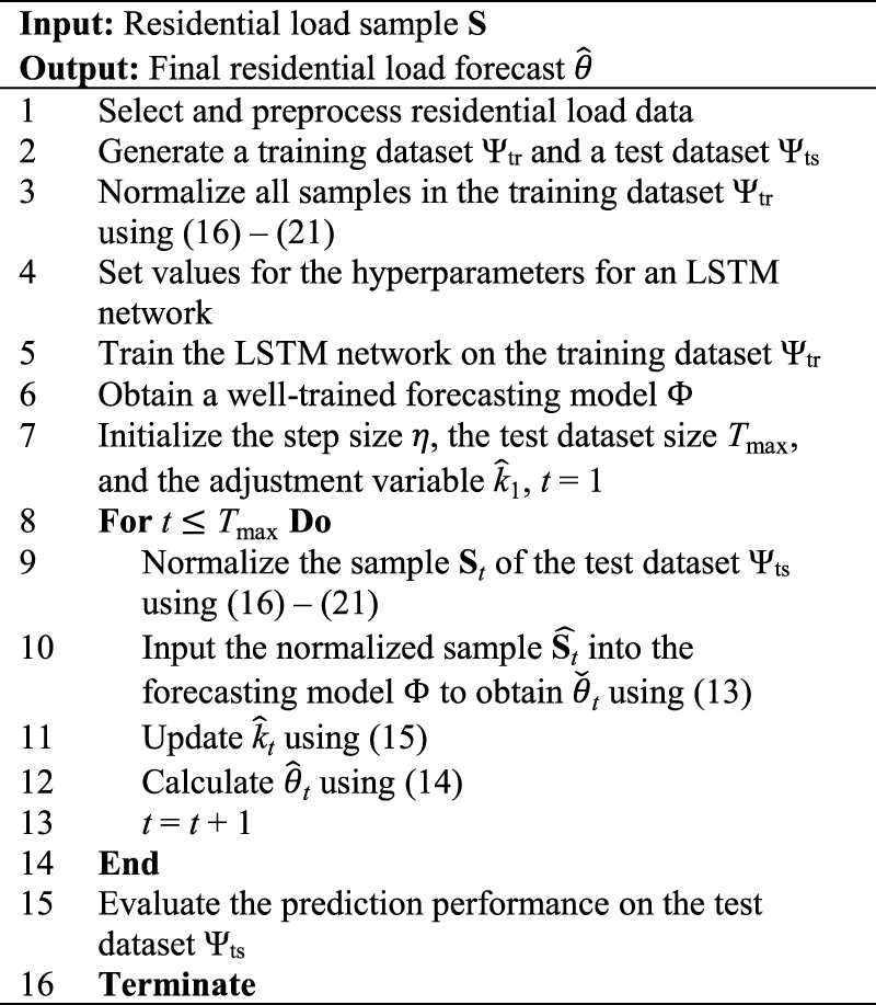
In order to perform adaptive residential load forecasting, an LSTM network is firstly well trained for each resident, and then it is applied with the modified DMD adjusting the forecasting error dynamically. In general, the proposed method goes through the following four steps sequentially to forecast residential load: 1) the input sample is formed; 2) the input sample is normalized and fed to the well trained LSTM network to obtain the intermediate forecast; 3) the adjustment variable of the modified DMD is updated; 4) the final forecast is computed by summing the adjustment variable and the intermediate forecast. The framework of integration of deep learning and dynamic mirror descent for adaptive individual residential load forecasting is shown in Figure 1, and the steps of LSTM and DMD integration are detailed in Algorithm 2.

FIGURE 1

FIGURE 1. Framework of integration of deep learning and dynamic mirror descent for adaptive individual residential load forecasting.

Algorithm 2. LSTM and DMD Integration for Adaptive Individual Residential Load Forecasting

4.2 Dataset description

The dataset used in this paper is from the Smart Metering Electricity Customer Behaviour Trials initiated by Commission for Energy Regulation in Ireland (Commission for Energy Regulation, 2012). The trials lasted from July 2009 to December 2010 with over 5000 Irish residential customers and small and medium enterprises (SMEs) participating. In the trials, there are 929 1-E-E customers, which means that they are all residential customers (1) with the controlled stimulus (E) and the controlled tariff (E). These customers are billed at the flat rate without any stimulus, and therefore are most representative because the majority of residential customers outside the trials are of this type. Among these 929 customers, 782 customers have a complete record of energy consumption throughout the trials. In this paper, 750 1-E-E customers with a complete record are randomly selected as the experiment dataset.

4.3 Experiment setup

The full data of a single residential customer is divided into a training dataset and a test dataset with a ratio of 9:1. So, for each resident, 90% of the data samples are used for training, while the rest of 10% are used for testing. In addition, as this paper is not focused on improving the prediction accuracy via the optimal network structure, hyperparameter fine-tuning is not conducted on the LSTM network. All the experiment parameters are presented in Table 2.

TABLE 2

TABLE 2. Experiment parameters of adaptive individual residential load forecasting based on deep learning and dynamic mirror descent.

5 Results and discussion

In this section, a performance comparison was firstly made between the proposed residential load forecasting method and a published benchmark method presented in Kong et al. (2019). It is noted that the benchmark method only uses the same LSTM network as the proposed method but does not apply any online learning method. RMSE and MAE are employed as the performance indexes for residential load forecasting, formulated as follows:

$\text{RMSE}=\sqrt{\frac{{\sum }_{\mathit{t}=1}^{\mathit{N}}{\left(\widehat{{\mathit{y}}_{\mathit{t}}}-{\mathit{y}}_{\mathit{t}}\right)}^2}{\mathit{N}}}(22)$

$\text{MAE}=\frac{{\sum }_{\mathit{t}=1}^{\mathit{N}}\left|\widehat{{\mathit{y}}_{\mathit{t}}}-{\mathit{y}}_{\mathit{t}}\right|}{\mathit{N}}(23)$

where $\widehat{{\mathit{y}}_{\mathit{t}}}$ is the forecasted value, ${\mathit{y}}_{\mathit{t}}$ is the real value, and N is the size of the test dataset. Furthermore, the effect of the parameter η of the modified DMD on the proposed residential load forecasting method was investigated. In this paper, the adjustment variable is initialised as 0.

5.1 Performance analysis of adaptive individual residential load forecasting

A performance comparison was conducted between the proposed and benchmark methods in terms of prediction accuracy. In this case, the parameter η of the modified DMD is set as 1.0 × 10⁻⁵, 1.0 × 10⁻⁴, 1.0 × 10⁻³, 1.0 × 10⁻², 1.0 × 10⁻¹, and 1.0×10⁰ respectively, and the optimal forecasting result obtained is regarded as the result of the proposed method. The results of both methods are presented in Table 3.

TABLE 3

TABLE 3. Residential load forecasting results of the proposed and benchmark methods.

It is noted that Table 3 describes the average RMSE and MAE of all the residents. In Table 3, the proposed method performs much better than the benchmark method, in terms of both RMSE and MAE. Besides, the improvement percentage of MAE is higher than that of RMSE, because MAE and RMSE indicate the forecasting performance from two different perspectives. To be specific, MAE, which reflects the mean of errors, regards every error equally and averages all the errors, while RMSE, which reflects the fluctuation of errors, strengthens the large error and weakens the small error.

The reason for the significant performance improvement of the proposed method can be explained as follows. As the adjustment variable ${\widehat{k}}_t$ of the modified DMD is capable to update itself based on the errors between the forecasts and the real measurements of the previous time steps, the proposed method can effectively adjust the intermediate forecast ${\stackrel{\mathrm{ˇ}}{\theta }}_{\mathit{t}}$ of the current time step to obtain the final forecast ${\widehat{\theta }}_{\mathit{t}}$.

In addition, Figure 2 presents the RMSE and MAE reduction of the proposed method across all the residents compared to the benchmark method, while Figure 3 presents the statistics of improvement percentage of the proposed method compared to the benchmark method.

FIGURE 2

FIGURE 2. RMSE and MAE reduction of the proposed method compared to the benchmark method.

FIGURE 3

FIGURE 3. Statistics of improvement percentage of the proposed method compared to the benchmark method.

In Figure 2, it can be clearly seen that the proposed method achieves different levels of improvements on a large number of residents. More specifically, some residents receive significant RMSE and MAE reductions (e.g., from 0.4 to 1.0), but others only receive slight RMSE and MAE reductions (e.g., from 0.01 to 0.05). It is also noted that some residents obtain an RMSE decrease but an MAE increase, while others obtain the opposite result. Besides, there is no performance difference between the proposed and benchmark methods for a few residents. This demonstrates that the modified DMD fails to effectively adjust the forecasting error over time, mainly because of the great complexity of these residential load profiles.

In Figure 3, there are totally 555 + 116 + 62 + 5 = 738 residents with an RMSE reduction, which account for 738/750 = 98.4% of all residents. Among them, most residents obtain an RMSE reduction of less than 20%, which account for (555 + 116)/750 = 89.47%. Besides, only five residents obtain an RMSE reduction of even more than 60%. Similarly, a total of 443 + 87 + 85 + 17 = 632 residents receive an MAE reduction, which account for 632/750 = 84.27%. Among them, most residents obtain an MAE reduction of less than 20%, which account for (443 + 87)/750 = 70.67%. Only 17 residents obtain an MAE reduction of even more than 60%. It is also noted that 118 residents fail to obtain an MAE reduction, while only 12 residents fail to obtain an RMSE reduction. This fact indicates that the proposed method tends to decrease RMSE in comparison with MAE.

Furthermore, Figure 4 shows the load profiles of a random resident forecasted by the proposed and benchmark methods during a random week (Monday 29/11/2010—Sunday 5/12/2010). It is obvious in Figure 4 that the forecasted load profile of the proposed method is much closer to the real load profile than that of the benchmark method. To be specific, when a dramatic increase or decrease of the residential load occurs, the proposed method can capture the change rapidly. Also, it can track the residential load stably, when the residential load only fluctuates slightly. By contrast, the benchmark method is unable to forecast accurately, when the residential load changes significantly over time.

FIGURE 4

FIGURE 4. Load profiles of the proposed and benchmark methods (Resident 3844).

5.2 Effect of parameter η on performance of adaptive individual residential load forecasting

As the parameter η plays an important role in the modified DMD, its effect on the forecasting performance of the proposed method was further investigated. Figure 5 depicts the MAE and RMSE reduction of the proposed method across all residents compared to the benchmark method, when the modified DMD is applied with different values of the parameter η.

FIGURE 5

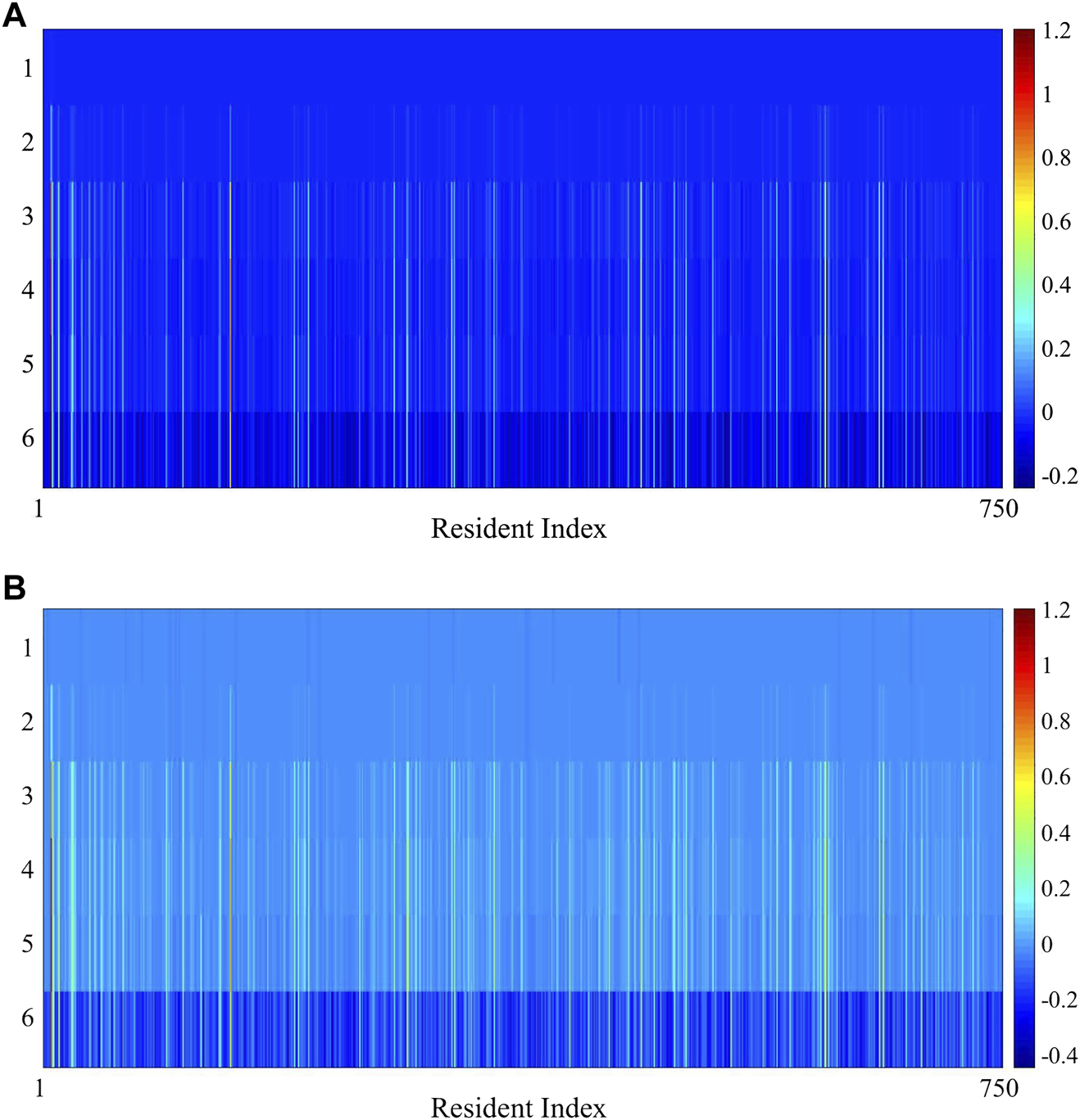
FIGURE 5. Effect of parameter η on the forecasting performance of the proposed method: 1) η = 1.0 × 10⁻⁵, 2) η = 1.0 × 10⁻⁴, 3) η = 1.0 × 10⁻³, 4) η = 1.0 × 10⁻², 5) η = 1.0 × 10⁻¹, 6) η = 1.0×10⁰. (A) MAE reduction. (B) RMSE reduction.

It can be clearly seen in Figure 5A that the proposed method has the worst performance when η is 1.0×10⁰, because a large number of residents fail to receive an MAE reduction. However, when η is 1.0 × 10⁻¹, 1.0 × 10⁻², and 1.0 × 10⁻³, the proposed method performs much better, because a majority of residents receive different MAE reductions. Only a small amount of residents receive an MAE reduction, when η is 1.0 × 10⁻⁴ and 1.0 × 10⁻⁵. It is also noted that there are a variety of trends of MAE reductions among all the residents as η changes from 1.0×10⁰ to 1.0 × 10⁻⁵. Likewise, in Figure 5B, in terms of RMSE, the proposed method has the worst performance when η is 1.0×10⁰, but performs much better when η is 1.0 × 10⁻¹, 1.0 × 10⁻², and 1.0 × 10⁻³. Only a small number of residents obtain an RMSE reduction, when η is 1.0 × 10⁻⁴ and 1.0 × 10⁻⁵. Besides, different trends of RMSE reductions can be seen among all the residents, as η changes from 1.0×10⁰ to 1.0 × 10⁻⁵.

The reason for the poor forecasting performance of the proposed method, when η is too small or too large, can be explained as follows. In (15), if η is too small, the deviation between the real measurement and the final forecast at the current time step cannot be accumulated effectively in the adjustment variable at the next time step. Thus, the modified DMD is unable to adjust the intermediate forecast properly over time. But, if η is too large, the deviation between the real measurement and the final forecast at the current time step accounts for a large proportion in the adjustment variable at the next time step, significantly weakening the accumulation of the deviations of the previous time steps. Therefore, the modified DMD fails to track the forecasting error accurately over time.

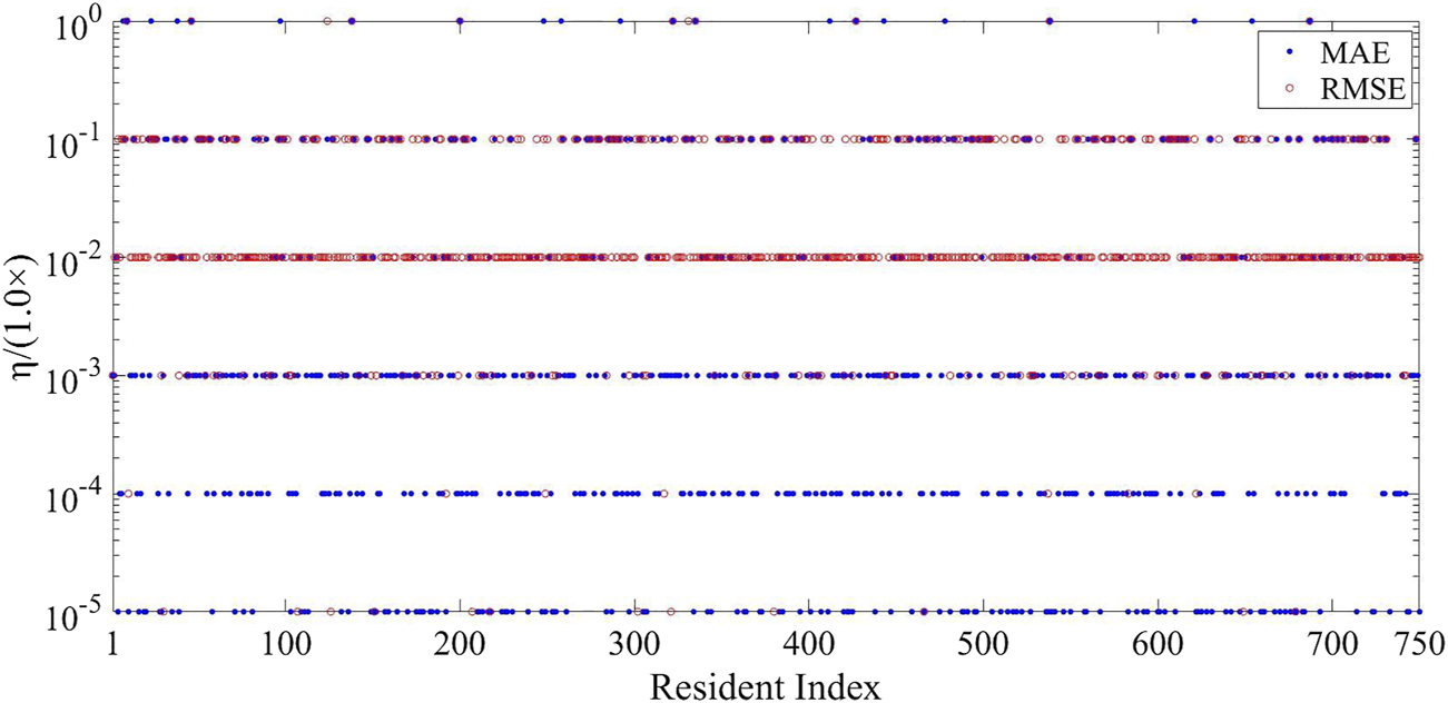
Furthermore, Figure 6 shows the optimal values of the parameter η when the proposed method achieves the best performance in terms of RMSE and MAE respectively. It is obvious in Figure 6 that the proposed method rarely achieves the minimum MAE value when η is 1.0×10⁰ and 1.0 × 10⁻⁵. However, it is capable to achieve the minimum MAE value on a large amount of residents when η is 1.0 × 10⁻³ and 1.0 × 10⁻⁴. Similarly, the proposed method is able to achieve the minimum RMSE value only on a few residents when η is 1.0×10⁰ and 1.0 × 10⁻⁵. But, it achieves the minimum RMSE value on a majority of residents when η is 1.0 × 10⁻¹ and 1.0 × 10⁻². As MAE and RMSE measure errors from two perspectives, the optimal values of η are different, when the proposed method achieves the minimum MAE and RMSE values on a single resident.

FIGURE 6

FIGURE 6. Optimal values of parameter η for the proposed method to achieve the minimum RMSE and MAE values.

In addition, Figure 7 describes the load profiles of a random resident forecasted by the proposed method on a random day (Wednesday 22/12/2010) when the modified DMD is applied with different values of the parameter η, while Figure 8 describes the forecasting errors of the proposed method on this resident as the parameter η changes.

FIGURE 7

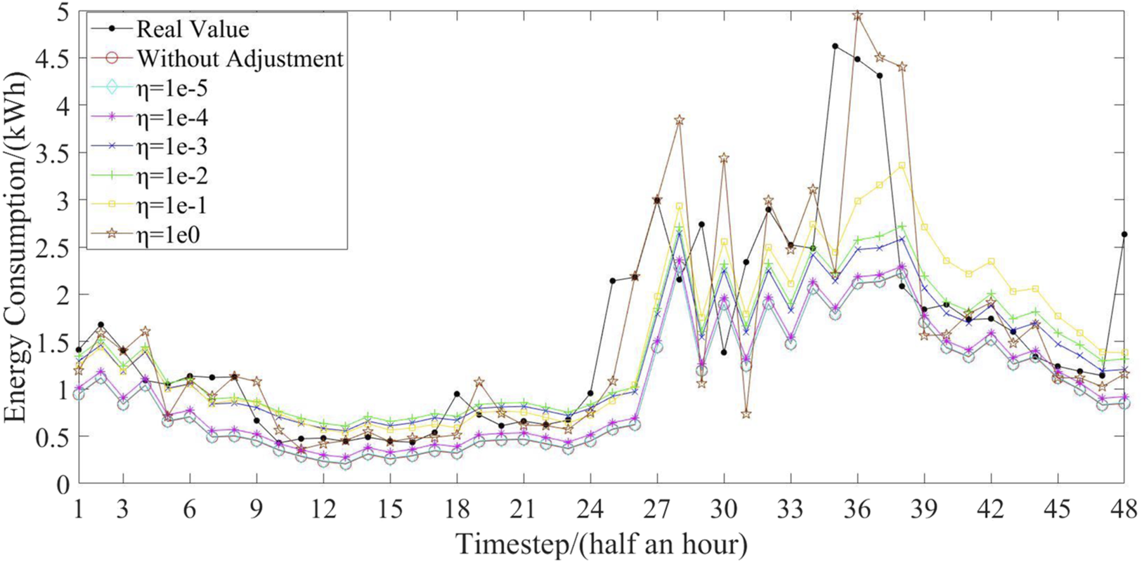
FIGURE 7. Load profiles of the proposed method for different values of parameter η (Resident 1425).

FIGURE 8

FIGURE 8. Forecasting errors of the proposed method for different values of parameter η (Resident 1425).

In Figure 7, the proposed method performs forecasting accurately at most time steps throughout the day, when η is 1.0 × 10⁻² and 1.0 × 10⁻³. By contrast, when η is 1.0 × 10⁻⁴ and 1.0 × 10⁻⁵, the forecasted load profiles of the proposed method are quite close to that of the benchmark method. When η is 1.0×10⁰ and 1.0 × 10⁻¹, there is a significant deviation between the real load profile and the forecasted load profiles of the proposed method at many time steps. This is mainly because a too small or too large value of η has a negative influence on the modified DMD. In Figure 8, MAE of the proposed method firstly decreases from η = 1.0 × 10⁻⁵ to η = 1.0 × 10⁻³, and then increases from η = 1.0 × 10⁻³ to η = 1.0×10⁰. The proposed method achieves the lowest MAE value of 0.3379 when η is 1.0 × 10⁻³. Similarly, RMSE of the proposed method firstly decreases from η = 1.0 × 10⁻⁵ to η = 1.0 × 10⁻², and then increases from η = 1.0 × 10⁻² to η = 1.0×10⁰. The proposed method achieves the lowest RMSE value of 0.5355 when η is 1.0 × 10⁻².

6 Conclusion

This paper has presented an adaptive individual residential load forecasting method, which integrates deep learning and dynamic mirror descent to address the issue of great volatility of individual residential load. The original DMD is modified to become feasible for dynamic residential load forecasting. Besides, a detailed feature expression strategy is devised to provide the proposed method with sufficient information of energy consumption at each time step. The experimental results have shown that the proposed method has improved the prediction accuracy substantially by 9.1% in RMSE and 11.6% in MAE, in comparison with the published benchmark method. In addition, the effect of the parameter η of the modified DMD on the proposed method is further explored, and the comparison results have indicated that the optimal value of η can be found out to achieve the maximum performance improvement.

Future work will focus on fine-tuning techniques to combine with deep learning and explore their effects on residential load forecasting. Optimization techniques will also be applied to search for the optimal value of the parameter η of the modified DMD in a continuous space in our future work.

Data availability statement

Publicly available datasets were analyzed in this study. This data can be found here: https://www.ucd.ie/issda/data/commissionforenergyregulationcer.

Author contributions

FH: responsible for investigation, conceptualization, methodology, formal analysis, visualization, original draft preparation, and review and editing. XW: responsible for review and editing, revision, project administration, and funding acquisition.

Funding

This work was funded by State Grid Corporation of China, under Grant Number 5700-202055267A-0-0–00 (Data Mining Technology of Potential High-Value Industrial Users for Data Operations).

Conflict of interest

The authors declare that the research was conducted in the absence of any commercial or financial relationships that could be construed as a potential conflict of interest.

Publisher's note

All claims expressed in this article are solely those of the authors and do not necessarily represent those of their affiliated organizations, or those of the publisher, the editors and the reviewers. Any product that may be evaluated in this article, or claim that may be made by its manufacturer, is not guaranteed or endorsed by the publisher.

References

Alhussein, M., Aurangzeb, K., and Haider, S. I. (2020). Hybrid CNN-LSTM model for short-term individual household load forecasting. IEEE Access 8, 180544–180557. doi:10.1109/ACCESS.2020.3028281

CrossRef Full Text | Google Scholar

Campos, B. P., and da Silva, M. R. D. (2016). “Demand forecasting in residential distribution feeders in the context of smart grids,” in Proceedings of the 2016 12th IEEE International Conference on Industry Applications (INDUSCON), 20-23 November 2016. (Curitiba, Brazil: IEEE). doi:10.1109/INDUSCON.2016.7874464

CrossRef Full Text | Google Scholar

Chen, X., Liu, X., Wang, Y., Gales, M. J. F., and Woodland, P. C. (2016). Efficient training and evaluation of recurrent neural network language models for automatic speech recognition. IEEE/ACM Trans. Audio Speech Lang. Process. 24 (11), 2146–2157. doi:10.1109/TASLP.2016.2598304

CrossRef Full Text | Google Scholar

Commission for Energy Regulation (CER) (2012). Cmmission for energy regulation (CER). Available at: https://www.ucd.ie/issda/data/commissionforenergyregulationcer/.

Google Scholar

Dinesh, C., Makonin, S., and Bajic, I. V. (2019). Residential power forecasting using load identification and graph spectral clustering. IEEE Trans. Circuits Syst. II 66 (11), 1900–1904. doi:10.1109/TCSII.2019.2891704

CrossRef Full Text | Google Scholar

Gan, D., Wang, Y., Zhang, N., and Zhu, W. (2017). Enhancing short-term probabilistic residential load forecasting with quantile long-short-term memory. J. Eng. 2017 (14), 2622–2627. doi:10.1049/joe.2017.0833

CrossRef Full Text | Google Scholar

Goehry, B., Goude, Y., Massart, P., and Poggi, J. (2020). Aggregation of multi-scale experts for bottom-up load forecasting. IEEE Trans. Smart Grid 11 (3), 1895–1904. doi:10.1109/TSG.2019.2945088

CrossRef Full Text | Google Scholar

Hall, E. C., and Willett, R. M. (2015). Online convex optimization in dynamic environments. IEEE J. Sel. Top. Signal Process. 9 (4), 647–662. doi:10.1109/JSTSP.2015.2404790

CrossRef Full Text | Google Scholar

Hossen, T., Nair, A. S., Chinnathambi, R. A., and Ranganathan, P. (2018). “Residential load forecasting using deep neural networks (DNN),” in Proceedings of the 2018 North American Power Symposium (NAPS), 9-11 September 2018 (Fargo, ND, USA: IEEE). doi:10.1109/NAPS.2018.8600549

CrossRef Full Text | Google Scholar

Humeau, S., Wijaya, T. K., Vasirani, M., and Aberer, K. (2013). “Electricity load forecasting for residential customers: Exploiting aggregation and correlation between households,” in Proceedings of the 2013 Sustainable Internet and ICT for Sustainability (SustainIT), 30-31 October 2013 (Palermo, Italy: IEEE). doi:10.1109/SustainIT.2013.6685208

CrossRef Full Text | Google Scholar

Kong, W., Dong, Z., Jia, Y., Hill, D. J., Xu, Y., and Zhang, Y. (2019). Short-term residential load forecasting based on LSTM recurrent neural network. IEEE Trans. Smart Grid 10 (1), 841–851. doi:10.1109/TSG.2017.2753802

CrossRef Full Text | Google Scholar

Kong, W., Dong, Z., Luo, F., Meng, K., Zhang, W., Wang, F., et al. (2017). “Effect of automatic hyperparameter tuning for residential load forecasting via deep learning,” in Proceedings of the 2017 Australasian Universities Power Engineering Conference (AUPEC), 19-22 November 2017 (Melbourne, VIC, Australia: IEEE). doi:10.1109/AUPEC.2017.8282478

CrossRef Full Text | Google Scholar

Ledva, G. S., Balzano, L., and Mathieu, J. L. (2015). “Inferring the behavior of distributed energy resources with online learning,” in Proceedings of the 2015 53rd Annual Allerton Conference on Communication, Control, and Computing (Allerton), 29 September - 2 October 2015 (Monticello, IL, USA: IEEE). doi:10.1109/ALLERTON.2015.7447003

CrossRef Full Text | Google Scholar

Ledva, G. S., Balzano, L., and Mathieu, J. L. (2018). Real-time energy disaggregation of a distribution feeder's demand using online learning. IEEE Trans. Power Syst. 33 (5), 4730–4740. doi:10.1109/TPWRS.2018.2800535

CrossRef Full Text | Google Scholar

Lin, W., Wu, D., and Boulet, B. (2021). Spatial-temporal residential short-term load forecasting via graph neural networks. IEEE Trans. Smart Grid 12 (6), 5373–5384. doi:10.1109/TSG.2021.3093515

CrossRef Full Text | Google Scholar

Marinescu, A., Dusparic, I., Harris, C., Cahill, V., and Clarke, S. (2014). “A dynamic forecasting method for small scale residential electrical demand,” in Proceedings of the 2014 International Joint Conference on Neural Networks (IJCNN), 6-11 July 2014 (Beijing, China: IEEE). doi:10.1109/IJCNN.2014.6889425

CrossRef Full Text | Google Scholar

Marinescu, A., Harris, C., Dusparic, I., Clarke, S., and Cahill, V. (2013). “Residential electrical demand forecasting in very small scale: An evaluation of forecasting methods,” in Proceedings of the 2013 2nd International Workshop on Software Engineering Challenges for the Smart Grid (SE4SG), 18 May 2013 (San Francisco, CA, USA: IEEE). doi:10.1109/SE4SG.2013.6596108

CrossRef Full Text | Google Scholar

Oprea, S. V., and Bara, A. (2019). Machine learning algorithms for short-term load forecast in residential buildings using smart meters, sensors and big data solutions. IEEE Access 7, 177874–177889. doi:10.1109/ACCESS.2019.2958383

CrossRef Full Text | Google Scholar

Paterakis, N. G., Tascikaraoglu, A., Erdinc, O., Bakirtzis, A. G., and Catalao, J. P. S. (2016). Assessment of demand-response-driven load pattern elasticity using a combined approach for smart households. IEEE Trans. Ind. Inf. 12 (4), 1529–1539. doi:10.1109/TII.2016.2585122

CrossRef Full Text | Google Scholar

Ponocko, J., and Milanovic, J. V. (2018). Forecasting demand flexibility of aggregated residential load using smart meter data. IEEE Trans. Power Syst. 33 (5), 5446–5455. doi:10.1109/TPWRS.2018.2799903

CrossRef Full Text | Google Scholar

Quilumba, F. L., Lee, W. J., Huang, H., Wang, D. Y., and Szabados, R. L. (2015). Using smart meter data to improve the accuracy of intraday load forecasting considering customer behavior similarities. IEEE Trans. Smart Grid 6 (2), 911–918. doi:10.1109/TSG.2014.2364233

CrossRef Full Text | Google Scholar

Sajjad, I. A., Chicco, G., and Napoli, R. (2016). Definitions of demand flexibility for aggregate residential loads. IEEE Trans. Smart Grid 7 (6), 2633–2643. doi:10.1109/TSG.2016.2522961

CrossRef Full Text | Google Scholar

Shi, H., Xu, M., and Li, R. (2018). Deep learning for household load forecasting-A novel pooling deep RNN. IEEE Trans. Smart Grid 9 (5), 5271–5280. doi:10.1109/TSG.2017.2686012

CrossRef Full Text | Google Scholar

Stephen, B., Tang, X., Harvey, P. R., Galloway, S., and Jennett, K. I. (2017). Incorporating practice theory in sub-profile models for short term aggregated residential load forecasting. IEEE Trans. Smart Grid 8 (4), 1591–1598. doi:10.1109/TSG.2015.2493205

CrossRef Full Text | Google Scholar

Tolosana, R., Vera-Rodriguez, R., Fierrez, J., and Ortega-Garcia, J. (2018). Exploring recurrent neural networks for on-line handwritten signature biometrics. IEEE Access 6, 5128–5138. doi:10.1109/ACCESS.2018.2793966

CrossRef Full Text | Google Scholar

Vossen, J., Feron, B., and Monti, A. (2018). “Probabilistic forecasting of household electrical load using artificial neural networks,” in Proceedings of the 2018 IEEE International Conference on Probabilistic Methods Applied to Power Systems (PMAPS ), 24-28 June 2018 (Boise, ID, USA: IEEE). doi:10.1109/PMAPS.2018.8440559

CrossRef Full Text | Google Scholar

Wang, L., Mao, S., Wilamowski, B. M., and Nelms, R. M. (2020). Ensemble learning for load forecasting. IEEE Trans. Green Commun. Netw. 4 (2), 616–628. doi:10.1109/TGCN.2020.2987304

CrossRef Full Text | Google Scholar

Wang, Y., Chen, Q., Sun, M., Kang, C., and Xia, Q. (2018). An ensemble forecasting method for the aggregated load with subprofiles. IEEE Trans. Smart Grid 9 (4), 3906–3908. doi:10.1109/TSG.2018.2807985

CrossRef Full Text | Google Scholar

Welikala, S., Dinesh, C., Ekanayake, M., Godaliyadda, B., Ekanayake, R. I., and Ekanayake, J. (2019). Incorporating appliance usage patterns for non-intrusive load monitoring and load forecasting. IEEE Trans. Smart Grid 10 (1), 448–461. doi:10.1109/TSG.2017.2743760

CrossRef Full Text | Google Scholar

Wijaya, T. K., Vasirani, M., Humeau, S., and Aberer, K. (2015). “Cluster-based aggregate forecasting for residential electricity demand using smart meter data,” in Proceedings of the 2015 IEEE International Conference on Big Data (Big Data), 29 October - 1 November 2015 (Santa Clara, CA, USA: IEEE). doi:10.1109/BigData.2015.7363836

CrossRef Full Text | Google Scholar

Wu, D., Wang, B., Precup, D., and Boulet, B. (2020). Multiple kernel learning-based transfer regression for electric load forecasting. IEEE Trans. Smart Grid 11 (2), 1183–1192. doi:10.1109/TSG.2019.2933413

CrossRef Full Text | Google Scholar

Xie, G., Chen, X., and Weng, Y. (2018). An integrated Gaussian process modeling framework for residential load prediction. IEEE Trans. Power Syst. 33 (6), 7238–7248. doi:10.1109/TPWRS.2018.2851929

CrossRef Full Text | Google Scholar

Xu, J., Meng Yue, M., Katramatos, D., and Yoo, S. (2016). “Spatial-temporal load forecasting using AMI data,” in Proceedings of the 2016 IEEE International Conference on Smart Grid Communications (SmartGridComm), 6-9 November 2016 (Sydney, NSW, Australia: IEEE). doi:10.1109/SmartGridComm.2016.7778829

CrossRef Full Text | Google Scholar

Zheng, J., Chen, X., Yu, K., Gan, L., Wang, Y., and Wang, K. (2018). “Short-term power load forecasting of residential community based on GRU neural network,” in Proceedings of the 2018 International Conference on Power System Technology (POWERCON), 6-8 November 2018 (China: GuangzhouIEEE). doi:10.1109/POWERCON.2018.8601718

CrossRef Full Text | Google Scholar

Zhou, D., Balandat, M., and Tomlin, C. (2016). “A Bayesian perspective on residential demand response using smart meter data,” in Proceedings of the 2016 54th Annual Allerton Conference on Communication, Control, and Computing (Allerton), 27-30 September 2016 (Monticello, IL, USA: IEEE). doi:10.1109/ALLERTON.2016.7852373

CrossRef Full Text | Google Scholar

Zou, M., Fang, D., Harrison, G., and Djokic, S. (2019). “Weather based day-ahead and week-ahead load forecasting using deep recurrent neural network,” in Proceedings of the 2019 IEEE 5th International forum on Research and Technology for Society and Industry (RTSI), 9-12 September 2019 (Florence, Italy: IEEE). doi:10.1109/RTSI.2019.8895580

CrossRef Full Text | Google Scholar