Accurate prediction of remaining useful life for lithium-ion battery using deep neural networks with memory features

1 Introduction

Prognostics and health management (PHM) deals with forecasting potential failures in many different engineering application systems, including battery management systems. PHM is necessary for the reliable operation of the system and allows timely remedial action by predicting future failures. Remaining useful life (RUL) is when the state of health (SOH) is expected to remain above a minimum acceptable SOH relative to the current time. In the case of a lithium-ion (Li-ion) battery, RUL is measured in terms of remaining cycles before the capacity degrades to less than 70% of its rated capacity (Xing et al., 2013; Tarar et al., 2021a; Amir et al., 2022) or 80% of its rated capacity depending on the application.

Li-ion batteries are widely used in several everyday applications, including electric vehicles, household equipment, satellite applications, communications applications, and cell phones (Tarar et al., 2023). The widespread use of Li-ion batteries is mainly due to their superiority over other types of batteries. These advantages include long cycle life, high energy density, high power density, high output voltage, and low self-discharge rate (Stroe et al., 2016; Hu et al., 2017b; Meng et al., 2018; Tarar et al., 2021b).

When the Li-ion battery is repeatedly charged and discharged, the total capacity decreases over time, termed health degradation. Many factors contribute to this aging process. Solid electrolyte interface (SEI) film grows on the electrodes due to the movement of Li-ions during the first charge-discharge cycle (formation process). The SEI layer continues to grow slowly, causing capacity fade (Pinson and Bazant, 2012). In addition, overcharging at low temperatures causes lithium plating, as some Li-ions are reduced to lithium metal, which further causes capacity loss during the charging and discharging process (An et al., 2016). An increase in internal impedance is another cause of capacity fade.

The RUL is an important metric to gauge reliability in electronic systems. It also gives insight into the proactive maintenance of systems. For Li-ion batteries, RUL prediction also supports safety considerations. Battery failure may cause damage to the entire system, potentially leading to critical injuries and significant financial loss. For example, a battery malfunction in an electric vehicle can cause an explosion and other complications. In cell phones or laptops, battery failures may render a device useless; knowledge of when the battery will malfunction can be advantageous.

1.1 Related work

This section presents prior work on RUL prediction. The approaches to predicting RUL can be categorized into model-based methods and data-driven methods. Model-based approaches utilize electrochemical principles, dynamic models, and equivalent circuit models. (Xiong et al., 2017) utilized electrochemical impedance spectroscopy (EIS) and proposed a method to identify degradation behavior. (Xu and Chen. 2017) proposed a state-space model utilizing expectation-maximization (EM) and extended Kalman filter (EKF) for RUL prediction. (Pinson and Bazant, 2012) introduced a single particle model to explain degradation in capacity, focusing on the growth of the SEI layer. (Hu et al., 2017a) utilized a reduced-form electrochemical model by proposing a moving horizon estimation framework (MHE). Even though model-based approaches give us a basic understanding of the dynamics of electrochemical reactions inside a battery, they are computationally expensive. Moreover, the parameters depend on operating conditions, so the model has limited applicability.

Because of the drawbacks and limitations of model-based approaches, data-driven approaches have received substantial attention recently. The advancements in machine and deep learning techniques and their non-reliance on inherent electrochemical dynamics make them an attractive alternative. Numerous machine learning and deep learning algorithms have been investigated such as the auto-regression model (Song et al., 2017), relevance vector machine (RVM) (Yuchen et al., 2018), Gaussian process regression (GP-regression) (Liu et al., 2013) and support vector machine (SVM) (Dong et al., 2014). Neural networks have proved efficient because of their nonlinear modeling capability (Wu et al., 2016; Tarar et al., 2022). Sequential dependency networks, such as recurrent neural networks (RNNs), are widely used (Liu et al., 2010; Sbarufatti et al., 2017; Zhang et al., 2022) proposed a prediction framework based on a combination of offline global models developed by different machine learning methods and cell-individualized models that were online adapted. (Hu et al., 2020) provided a timely and comprehensive review of the battery lifetime prognostic technologies, focusing on recent advances in model-based, data-driven, and hybrid approaches. These approaches’ details, advantages, and limitations were presented, analyzed, and compared.

A novel hybrid method is proposed (Xu et al., 2022) to predict battery capacity degradation trajectory, which combines physics-based and data-driven approaches in three steps: hybrid feature extraction, clustering with data augmentation, and training a deep neural network. The method provides accurate predictions with only 20% training data and is robust to noisy input. Validation results show mean absolute percentage errors below 2.5% for capacity degradation trajectory and 6.5% for remaining useable cycle life under different aging conditions. (Deng et al., 2022) use battery aging data to recognize degradation patterns and improve the state of health (SOH) estimation accuracy using transfer learning. Four discharge capacity curve features are extracted, with two distinct degradation patterns and two used for SOH estimation. Long short-term memory (LSTM) network achieves the best SOH estimation accuracy compared to other algorithms, and degradation pattern recognition and transfer learning methods further improve accuracy to mean MAE and RMSE values of 0.94% and 1.13%.

Jiang et al. (2021) proposed a reliable cycling aging prediction based on a data-driven model to address the urgent issue of adaptive and early prediction of lithium-ion batteries’ remaining useful life. First, a multi-kernel relevance vector machine (RVM) model with two alternative kernel functions was built to improve the learning and generalization capabilities of the traditional RVM. Next, the kernel and weight parameters were determined using the particle swarm optimization approach. A similarity criterion of the battery capacity curves is then provided to filter offline battery data for model training to accomplish early life prediction. For model training and verification, battery cycling aging data from two different types of batteries under various aging conditions were employed. Ren et al. (2018) proposed an integrated deep learning approach in which 21-dimensional features extracted from the National Aeronautics and Space Administration (NASA) dataset are fused by an auto-encoder that reduces their dimensionality to 15. The reduced 15-dimensional features are then fed to a deep neural network (DNN) model for RUL prediction.

1.2 Contributions

The capacity of the battery degrades over charge-discharge cycles. In data-driven approaches, various features extracted from the measured data exhibit valuable patterns that can be exploited to predict the battery’s RUL. These trends can be exploited in a time series analysis using features spanning multiple cycles. However, these memory-based features that span multiple cycles have rarely been used.

With a growing trend of using deep neural networks in such problems, domain knowledge-based features are also declining, and researchers bank on the power of neural networks to extract features from the data. Feature engineering is an important aspect where domain knowledge plays an important role. A careful presentation of the data can help identify the trends in the data and can be an important step in validating the dataset. Furthermore, the identified features are used with memory to predict RUL by introducing a window spanning multiple cycles capturing features of the previous n cycles. The main contributions of this research are as follows

1. This paper developed a novel framework—DNN with memory features (DNNwMF)—to accurately predict the RUL of Li-ion batteries using features of current and previous n cycles.

2. The proposed DNNwMF is also compared with logistic regression and SVM models.

3. The optimal value of n (n_opt)is computed, giving the minimum testing loss.

4. The effect of increasing C-rate and temperature on the optimal value of n is explored.

5. The input dimension increases significantly if n_opt number of cycles are used. Therefore, a framework, namely, an autoencoder and DNN with memory features (ADNNwMF), is employed to considerably reduce the number of dimensions and optimization parameters in the online training phase without much loss in RUL prediction accuracy.

Incorporating memory in features in such a way for batteries has not been found in the literature. Memory-based features in a simple deep neural network are used rather than RNN or LSTM. RNN and LSTM networks are more complex and take longer to train than DNN. LSTM networks also require more memory to train and can easily overfit. Moreover, dropout is much harder to implement in LSTM. In addition, LSTM is sensitive to different random weight initializations. Also, LSTM processes time-dependent data, so using the extracted features might not be a good way to feed to an LSTM network. Instead, providing sequential raw information is a better approach with the LSTM network. These limitations make it challenging to find the optimal value of n, for which the proposed method is used. Hence, the proposed method allows for finding an optimal window to incorporate memory, which has not been done for Li-on battery datasets.

The generalizability of the results is another crucial aspect often overlooked in data-driven approaches. The design of experiments for dataset creation is constrained because only a few attributes, like charging profiles, discharging profiles, temperature, and humidity, are changed to build a dataset. Therefore, datasets capture different degradation mechanisms; hence, a data-driven technique optimized for a dataset may not work if the dataset is changed. In order to confirm the generalizability of the results, two different datasets, a) from the Prognostic Center of excellence of National Aeronautics and Space Administration (NASA) and b) the Center for Advanced Life Cycle Engineering (CALCE) dataset provided by the University of Maryland College Park are used to validate the results. For these datasets, the tests have been performed in different conditions. For instance, all the tests for NASA’s dataset are run at room temperature, whereas the CALCE dataset has 22 different test conditions that vary in temperature, C-rate, and the time interval between cycles.

The next section describes the proposed framework and problem formulation. Section 3 presents and analyzes the experimental results and Section 4 concludes this paper.

2 Proposed deep learning with memory features framework

Figure 1 shows the proposed DNNwMF and ADNNwMF frameworks of DNNs with memory features with and without auto-encoder. Features are extracted from the dataset. In Figure 1A features of the last n cycles are used without auto-encoder, whereas in Figure 1B the memory-based features are fused, and their dimensionality is reduced using autoencoder. These low-dimensional fused features are then fed to the DNN model for RUL prediction.

FIGURE 1

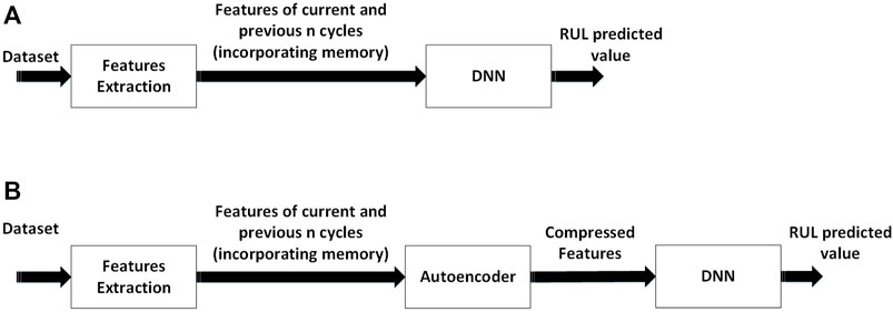
FIGURE 1. The proposed frameworks (A) DNN with memory features (DNNwMF) and (B) autoencoder with DNN with memory features (ADNNwMF).

The problem to be solved is as follows: given the i^th cycle features, xⁱ, and the features of previous n cycles {xⁱ, xⁱ⁻¹, xⁱ⁻², ……, xⁱ⁻ⁿ}, estimate the RUL, yⁱ, corresponding to the i^th cycle. The paper investigates whether the introduction of memory (expanding the feature set to previous n cycles) improves RUL prediction accuracy. Furthermore, the number of cycles to be used, n, is empirically optimized. The goal is to find the optimal window of the i^th and previous n cycle features to predict RUL as efficiently as possible.

2.1 Data set validation and feature extraction

Figure 2 shows one cycle of the most widely used constant current constant voltage (CC-CV) charge and discharge process.

FIGURE 2

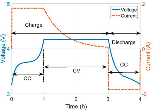
FIGURE 2. One cycle of constant current constant voltage (CC-CV) charge discharge process.

(a) Charging process: In the charging process, the first step is constant current (CC) charging, in which current is set to a constant value while voltage is raised to the maximum upper limit. After that, the voltage is kept at this constant value, called the constant voltage (CV) charging step. While the voltage is kept at the CV, the current drops to a certain threshold.

(b) Discharging process: This process consists entirely of CC discharging in which the voltage drops to the lower limit.

In typical experimental data, the charging and discharging processes described above are repeated until the battery reaches its end of life. In this paper, the NASA dataset (Saha and Goebel, 2019) and the Center for Advanced Life Cycle Engineering (CALCE) dataset provided by the University of Maryland (UMD) College Park have been used for RUL estimation. Features are extracted from the charging and discharging voltage and current profile from the two datasets.

When the battery goes through charge-discharge cycles, several degradation mechanisms occur, which include loss of lithium inventory, lithium plating, and metallic dendrites, negative electrode degradation, degradation in composite electrode, metal dissolution, positive electrode degradation in bulk, loss of active material, and increased impedance. These degradation mechanisms reduce the battery capacity, manifested in the shortening of the time it takes to reach upper and lower cutoff voltage during charging and discharging. Similarly, constant current charging time and constant current discharging time decrease over the cycles. Hence, these features can help extract helpful degradation patterns to help predict RUL.Figures 3, 4 shows the battery voltage and battery output current over time during multiple charge and discharge cycles of battery B0005 from the NASA data set.

FIGURE 3

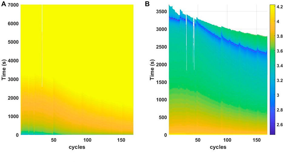
FIGURE 3. Battery voltage in relation to time and number of cycles during (A) charging and (B) discharging cycle.

FIGURE 4

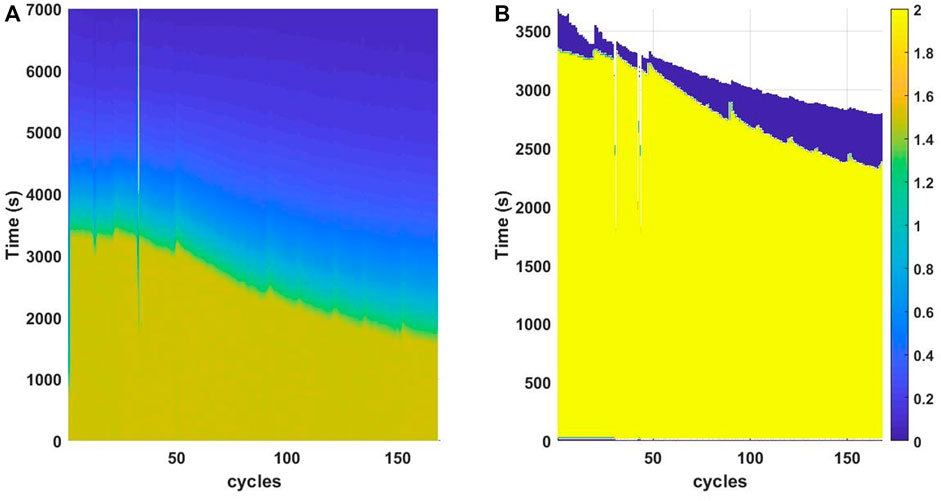
FIGURE 4. Battery output current in relation to time and number of cycles during (A) charging and (B) discharging cycle (absolute values are plotted, in actual the discharging current has negative values).

The figures visibly capture various trends as the battery ages and the number of cycles increases. This kind of plotting shows the variation of all these features over the charge-discharge process and how the trend varies over the number of cycles. For example, Figure 3 shows how the battery voltage varies over time during the charge-discharge cycle. During the CC phase in the charging cycle, as shown in Figure 3A, the battery voltage increases to its cut-off voltage, where it stays constant for the rest of the cycle; however, the time required to reach the cut-off voltage decreases with the number of cycles. Figure 3B demonstrates that the time to reach the lower cut-off voltage during the discharge phase decreases with the increasing number of cycles. Similarly, the CC charging and discharging time decrease as the number of cycles increases, as shown in Figure 4. Thus, clear patterns emerge as the battery ages, benefiting battery prognostics.

However, as the battery ages and its capacity fades, the collected samples in the charging and discharging process are different: 4,500–5,000 for newer and 700–800 for old batteries. Therefore, it is not feasible to use these data samples directly from the charge and discharge cycle into the prognostic framework without data pre-processing or a mechanism for feature extraction. To learn from this data, features are extracted from the charge and discharge cycle that can be used in RUL prognostics. The extracted features are as follows:

Upper Cut-off Voltage Time: During the charging process, the battery terminal voltage features are

$\begin{array}{c}\hfill \left(t_{\text{min}\left(i\right)},V_i\right),V_i⩾\text{upper\hspace{0.17em}cut}-\text{off\hspace{0.17em}voltage},\\ \hfill i=\mathrm{1,2,3},\dots ,m,\end{array}(1)$

where t_min(i) represents the time when the battery terminal voltage reaches the maximum value first, and V_i represents the value of the output voltage in the i_th cycle.

Constant Current Charging Time (CCCT): One of the output current features is CCCT which represents the time when the output current of the battery starts to drop,

$\begin{array}{c}\hfill \left(t_{\text{min}\left(i\right)},A_i\right),A_i⩽\text{constant\hspace{0.17em}current\hspace{0.17em}value},\\ \hfill i=\mathrm{1,2,3},\dots ,m,\end{array}(2)$

where A_i represents the current value in the i_th cycle. Maximum Charging Voltage Time: The time required to reach the maximum battery measured voltage is given as

$\left(t_{\text{max}},V_{\text{max}}\right)=\left\{\left(t_i,V_i|\text{max}\left(V_i\right)\right)\right\},i=\mathrm{1,2,3},\dots ,m,(3)$

where t_max is the time stamp for which the maximum voltage V_max is measured in the i_th cycle.

Constant Voltage Charging Time: The time for which the battery is charged at constant voltage

$\begin{array}{c}\hfill \left(t_{\text{min}\left(i\right)},V_i\right),V_i⩽\text{constant\hspace{0.17em}voltage\hspace{0.17em}value},\\ \hfill i=\mathrm{1,2,3},\dots ,m,\end{array}(4)$

where V_i represents the voltage value in the i_th cycle.

Minimum Discharging Voltage time: During the discharging process, the time for which the battery terminal voltage reaches its minimum voltage is given as

$\left(t_{\text{min}},V_{\text{min}}\right)=\left\{\left(t_i,V_i|\text{min}\left(V_i\right)\right)\right\},i=\mathrm{1,2,3},\dots ,m,(5)$

where t_min is the time to reach the minimum battery terminal voltage value V_min in the i_th cycle.

Constant Current Discharging Time: The time when the output current during the discharging phase starts to rise again is the constant current charging time given as

$\begin{array}{c}\hfill \left(t_{\text{min}\left(i\right)},A_i\right),A_i⩾-\text{constant\hspace{0.17em}current\hspace{0.17em}value},\\ \hfill i=\mathrm{1,2,3},\dots ,m,\end{array}(6)$

where t_min(i) represents the time and A_i represents the value of current in the i_th cycle.

Battery Capacity: Battery capacity, C, represents the discharge capacity available at each cycle. The discharge capacity feature is the product of the last two features (t_min(i), A_i), so it may seem unnecessary to include it. However, the experiments show accuracy loss with no significant reduction in the number of optimization parameters. Moreover, the optimal values of n obtained by excluding this feature are the same when including this feature. Also, because an autoencoder using the optimal value of n is employed, the redundancy of features is being taken care of.

2.2 Generating labels and data normalization

Prediction of RUL requires the true labels of RUL for the training phase. For this, the total number of battery charge and discharge cycles are calculated and assigned as the total cycle life L. Then, for the i^th charge and discharge cycle (0⩽i⩽n), RUL (y_i) is calculated as

$y_i=L+1-i.(7)$

Finally, x_i and y_i are combined to get the supervised data (x_i, y_i) where x_i is the input feature with label y_i. To mitigate any negative effects of different data ranges, data normalization is carried out to map each feature in an interval [0, 1] using the minimum-maximum normalization method on the input x_i.

2.3 Training DNN for RUL prediction

A DNN is employed with memory features that use the features of the last n cycles at the input. The DNN is a supervised learning model. The input is fed to the network along with the ground truth. The network processes input assigns weights to different inputs, and passes it through a nonlinear function to generate the mapping for the next layer. For instance, for the i^th hidden layer, its input is mapped as

${\mathbf{h}}^{\mathbf{i}}=\mathcal{f}\left(\mathbf{W}{\mathbf{h}}^{\mathbf{i}-\mathbf{1}}+\mathbf{b}\right),(8)$

where $\mathcal{f}$ is non-linear activation function, W is the weight matrix, b is the bias, and hⁱ⁻¹ is the output of the previous hidden layer. The output of the last layer is compared with the ground truth to form a loss function. During the training phase, the layers’ weights are optimized so that the loss function is minimized. The framework uses a DNN model consisting of four fully connected layers; the number of neurons in each layer is 10, 7, 4, and 1. The current DNN structure was picked based on the results of tuning the model. The number of hidden layers and the number of neurons in each hidden layer were varied, and the best results were used. The rectified linear unit (ReLu) function is used as an activation function for the intermediate hidden layers, and the sigmoid function is used as an activation function for the output layer. The network is then trained to minimize the root mean square error (RMSE) as the error (loss) metric given by

$\mathrm{R}\mathrm{M}\mathrm{S}\mathrm{E}=\sqrt{\left(\frac{1}{N_t}\right)\sum _{i=1}^{N_t}{\left({\widehat{y}}_i-y_i\right)}^2},(9)$

where N_t is the size of the training set. ${\widehat{y}}_i$ and y_i are the predicted value and the true value of sample i respectively.

2.4 Autoencoder

As the number of features in the DNNwMF framework increases, the number of optimization parameters also increases. Redundancies in the features also creep into the system. In such a scenario, an auto-encoder is used to reduce the dimensionality of the input features. An autoencoder is used instead of other compression algorithms, such as PCA, because the features have a nonlinear relationship to the cycle life. An autoencoder can compress the information better into low dimensional latent space, leveraging its capability to model complex nonlinear functions. Moreover, the autoencoder is better at feature fusion than PCA. PCA simply learns a linear transformation that projects the data into a different space, with the projection vectors determined by the data’s variance. Autoencoder is a neural network that tries to mimic the input and hence tries to learn an identity system (Gondara, 2016; Tarar and Khalid, 2021). It consists of an encoder-decoder pair. A fully connected autoencoder encodes the input vector x into a latent space representation as vector z using a transformation of the form

$\mathbf{z}=\mathcal{f}\left({\mathbf{W}}_e\mathbf{x}+{\mathbf{b}}_e\right),(10)$

where $\mathcal{f}$ is non-linear activation function, W_e is the weight matrix, and b_e is the bias at the encoder. Latent space representation z is then decoded into an output space $\tilde{\mathbf{x}}$ having the same dimensionality as x. This transformation also uses a similar mapping, that is,

$\tilde{\mathbf{x}}=\mathcal{f}\left({\mathbf{W}}_d\mathbf{z}+{\mathbf{b}}_d\right).(11)$

(W_e, W_d, b_e, b_d) are the weights optimized using a back propagation algorithm so that the error in the reconstruction is minimized.

Autoencoders are used for many applications, including feature extraction, feature fusion, dimensionality reduction, and denoising, to name a few. Here, the task is two-fold; dimensionality reduction and feature fusion. When the parameters above are optimized, the hidden neurons can be used to express the input, albeit with a reduced dimension. In this paper, autoencoders compress the high dimensional highly correlated features to low dimensional complex features as opposed to (Ren et al., 2018), which used autoencoder only to reduce the 21-dimensional features to 15-dimensional features. The autoencoder contains one hidden layer containing nine neurons. So the features were compressed to nine features. The input and output layers contain ((n_opt + 1) × 13) number of neurons.

3 Experimental details

3.1 Dataset

This paper used the Li-ion batteries data set from NASA’s Prognostic Center of excellence (PCoE) (Saha et al., 2009; Saha and Goebel, 2019) and the Center for Advanced Life Cycle Engineering (CALCE) dataset provided by the University of Maryland (UMD) College Park. The NASA dataset was collected under room temperature and rated conditions. B0005, B0006, B0007, and B0018 batteries were used to generate results. The total number of cycles, i.e., m, was 168 for batteries B0005, B0006, and B0007, while m = 132 for battery B0018. The CALCE dataset contains data from six vendors under twenty-two different test conditions of temperature, discharge C-rate, and rest time. Although the cycle datasets used in the paper contain batteries that only last a few hundred cycles, the developed method will work for batteries with longer cycle life ($>1000$ cycles). Also, it is pertinent to mention that the CALCE dataset contains battery life cycles closer to 1,000 cycles. Therefore, the developed method can be applied to batteries with any life cycle. Table 1 presents CALCE dataset test conditions used in the paper. For all test conditions of the CALCE dataset, the charging took place at 0.8 C.

TABLE 1

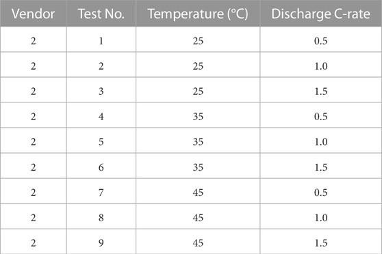
TABLE 1. UMDCALCE dataset test conditions used in this paper.

3.2 Feature extraction and data normalization

All the features explained in Section 2 were extracted for batteries from two datasets. Batteries B0005, B0006, and B0007 were used for training, and battery B0018 was used for testing from the NASA dataset. For the CALCE dataset, as each test condition contained three battery samples, two samples were used for training, and the remaining sample was used for testing. Thus, for nine test conditions shown in Table 1, nine separate models were trained using two samples, with the third sample used for testing. As there are 168 cycles for the batteries B0005, B0006, and B0007, RUL corresponding to i^th cycle is calculated as 169 − i. For battery B0018, i^th cycle RUL was calculated as 133 − i as it contains 132 cycles. The paper used a similar process for the CALCE dataset. The data were normalized using minimum-maximum normalization. As indicated previously, there were separately trained models for two datasets. In fact, for the CALCE dataset, there were nine trained models for the nine test conditions used in the paper. Training so many models may raise the question of why not a universal model is trained for both datasets. However, the two datasets contain batteries of different chemistries. Furthermore, the CALCE dataset comes from six different vendors with 22 different testing conditions. Each test condition triggers different degradation mechanisms. Hence, all these factors make it challenging to make a universal model even for the same dataset with different test conditions, let alone for different datasets. Thus, as will be seen from the results, the optimal value of n is different for different test conditions, indicating difficulty in obtaining a universal model.

3.3 Results and discussion

This subsection shows that without using memory features, an auto-encoder is not required. This section also presents the results of DNNwMF with different values of n and finds the optimal value n_opt. The optimal value of n refers to the number of previous cycles used with the current cycle to predict the RUL. For each value of n, training data is used to train the model. Within the training data, validation data is used to test the model, and the model is selected based on the minimum validation loss. The testing data is then used on the trained model, and RMSE (%) is obtained. This process is repeated for all the values of n. The optimal value of n is chosen for which the change in RMSE (%) starts to diminish (0.01% in this case). In other words, for each n, the optimal model is chosen using validation loss, with the optimal value of n chosen using the testing loss. The proposed DNNwMF is compared with logistic regression and SVM models, and the effect of increasing C rate and temperature on the optimal value n_opt is explored. The SVM benchmark used Gaussian Kernel Radial Basis Function (RBF) and the hyperparameters were optimized within the Regression Learner app in MATLAB to automate the selection of hyperparameter values. Finally, the results with ADNNwMF show that an autoencoder can be used to reduce the number of optimization parameters considerably without compromising accuracy. Stochastic gradient descent with RMSE as a loss function is used for all these cases during the training phase. After optimizing parameters during the training, RUL prediction results are verified using the testing set. The results are presented using RMSE (%), which is calculated as follows.

$\mathrm{R}\mathrm{M}\mathrm{S}\mathrm{E}\left(\%\right)=\sqrt{\left(\frac{1}{N_t}\right)\sum _{i=1}^{N_t}{\left(\frac{{\widehat{y}}_i-y_i}{y_i}\right)}^2}\times 100,(12)$

where N_t is the size of the training set. ${\widehat{y}}_i$ and y_i are the predicted and actual value of sample i, respectively.

3.3.1 Redundancy of auto-encoder without memory features

In the absence of memory features, using autoencoders is not required. Thus, when features of only one cycle are applied, the use of an autoencoder worsens the accuracy compared to a simple DNN, and the number of optimization parameters is also not reduced considerably.

Figure 5 shows the prediction results for battery B0018 using auto-encoder and DNN (ADNN) and DNN without memory (n = 0). These results show the true and predicted RUL on i^th cycle when features of i^th cycle are used. The vertical axis represents the normalized RUL values, and the horizontal axis represents the cycle number at which RUL is predicted. The black line shows the true normalized RUL values, the red line shows the predicted RUL values using ADNN, and the blue line shows the predicted RUL values using DNN only. The RMSE with ADNN is 11.34%, whereas the RMSE with DNN is 9.92%. The number of optimizing parameters is 214 and 254 for ADNN and DNN, respectively. This demonstrates that using an auto-encoder does not provide a significant gain in terms of the number of optimization parameters, and it results in a worse performance than a simple DNN.

FIGURE 5

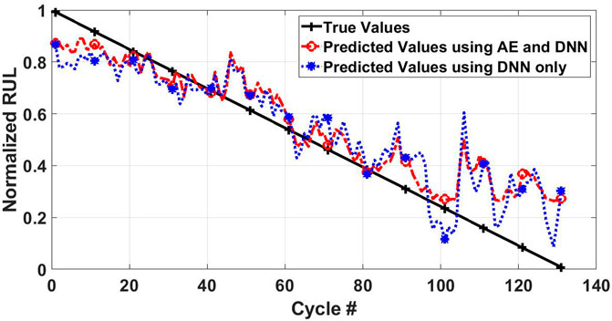
FIGURE 5. Prediction results for autoencoder & DNN without using memory features (n =0) in comparison with prediction results for DNN without using memory features (n =0).

3.3.2 Results with DNNwMF

The proposed framework uses features of the previous n cycles during the prediction process. To reiterate the point made in the last subsection, Table 2 compares the RMSE (%) and the number of parameters to optimize for ADNNwMF with DNNwMF for n ∈ {0, 1, 2}. This means that in order to predict RUL on i^th cycle, features of cycles [i, ⋯i − n] are used. It can be seen from Table 2 that DNNwMF predicts RUL more accurately as compared to ADNNwMF without having an extra processing step in the form of an autoencoder network, but it requires a larger number of parameters to optimize as the input features increase with n. Note that the number of features optimized by auto-encoder is not included as the feature compression with auto-encoder can be performed offline.

TABLE 2

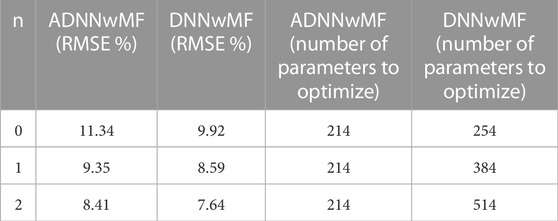
TABLE 2. RMSE(%) for n =0,1,2 for ADNNwMF and DNNwMF and corresponding number of optimization parameters.

As DNNwMF gives better prediction accuracy than ADNNwMF, the optimal n_opt value is found using DNNwMF. n and input features are increased to predict RUL using the DNNwMF framework. Table 3 shows the RMSE (%), change in RMSE, and the number of parameters to optimize for different values of n for the NASA dataset. It can be seen that as n increases, the prediction accuracy increases, and RMSE decreases. However, diminishing returns are obtained as n is increased, and the rate of change of the accuracy improvement slows considerably at higher values of n, as shown in Figure 6. At n = 17, the curve flattens and there is a very small decrease in RMSE, and so n = 17 is taken to be the optimal value n_opt. Figure 7 shows the battery B0018 prediction results using DNNwMF when n_opt(n = 17) is used. Table 4 compares the performance of DNNwMF with logistic regression and SVM, and it can be seen that DNNwMF outperforms both. If n increases, the model may run into an overfitting problem. However, in the cases addressed in this paper, the overfitting problem did not occur. Regardless, if needed, regularization techniques and dropout layers can be used to overcome the overfitting problem.

TABLE 3

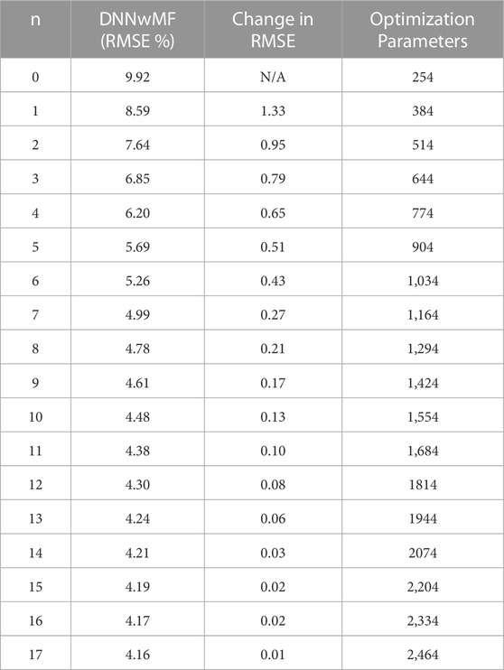
TABLE 3. RMSE% and change in RMSE with increase in value of n for DNNwMF and corresponding number of parameters to optimize.

FIGURE 6

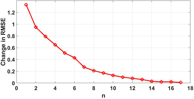
FIGURE 6. Change in RMSE for DNNwMF framework with the increase in n.

FIGURE 7

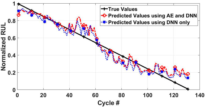
FIGURE 7. Prediction results for DNNwMF when features of n_opt =17 cycles are used in comparison with prediction results for ADNNwMF when features of n_opt =17 cycles are used.

TABLE 4

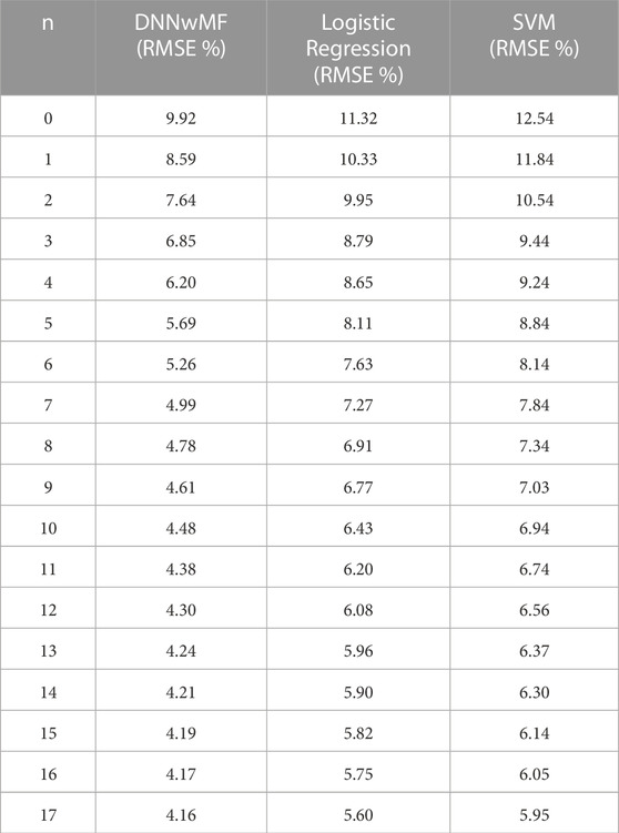
TABLE 4. Comparison of DNNwMF with logistic regression and SVM on NASA dataset.

3.4 Results on CALCE dataset

Table 5 shows the optimal value n_opt for each test condition for the CALCE dataset. It can be seen that increasing discharge C-rate and temperature increases the n_opt. Figure 8 shows the RMSE (%) for each test number of the CALCE dataset at n_opt for DNNwMF, logistic regression and SVM. DNNwMF outperforms both logistic regression and SVM.

TABLE 5

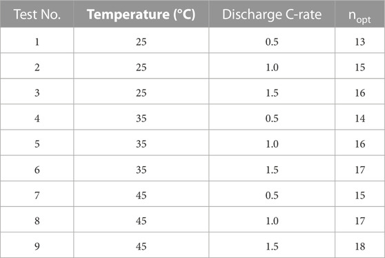
TABLE 5. Optimal n for each test condition for UMD CALCE dataset.

FIGURE 8

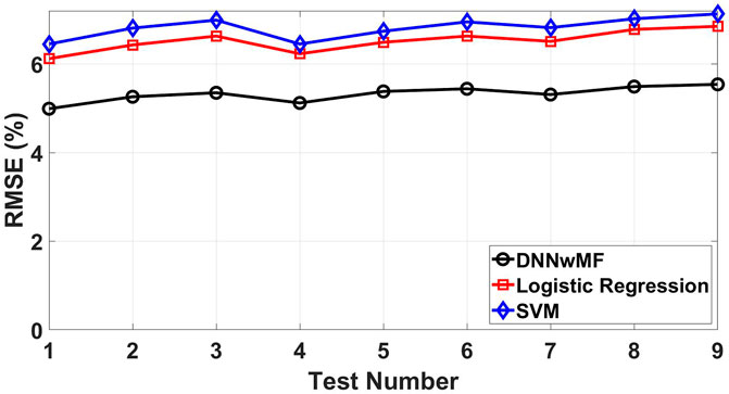
FIGURE 8. RMSE (%) vs. test number of UMD CALCE dataset.

Table 3 also shows that the number of parameters to optimize increases with the increase in n. For instance, for n = 17, the number of optimization parameters is an order of magnitude higher compared to n = 0. Thus, improved accuracy is achieved at the cost of computational complexity.

3.4.1 Results with ADNNwMF

Finally, an autoencoder is employed to reduce the number of parameters to optimize. The auto-encoder is used to compress the features to a much lower dimension. This reduces the number of optimization parameters significantly. For instance, for n = 17, the optimization parameters reduces from 2,464 to 214 when the features (13 × 18 dimensional) are encoded to a 9-dimensional feature set. Figure 7 shows the prediction results when encoding dimension of nine is used for n = n_opt = 17 which achieves an RMSE of 5.11%. Therefore, using an autoencoder reduces the feature dimensions and, consequently, the number of parameters to optimize but at the cost of accuracy. However, the proposed solution allows the flexibility to increase the encoding dimensions and achieves better accuracy. Table 6 compares the performance of ADNNwMF with a different number of encoding dimensions or the compressed features with auto-encoder. It can be seen that autoencoders are more efficient in exploiting the redundancy of features without significant loss in prediction accuracy and, at the same time, significantly reduce the number of optimization parameters (see Table 6). For instance, comparing the performance of DNNwMF with n = 8 with ADNNwMF with n = n_opt = 17 and encoding dimensions of 45, it can be seen that the DNNwMF achieves an RMSE of 4.78% with 2014 parameters whereas ADNNwMF achieves an RMSE of 4.74% with only 574 parameters to be optimized. From Table 6, it can be seen that by increasing the number of neurons in the encoding layer, the RMSE can be reduced. Table 6 also shows the performance in RMSE% of autoencoder with logistic regression (ALogReg) and autoencoder with SVM (ASVM). It can be seen that autoencoder with DNN (ADNN) outperforms both ALogReg and ASVM. Figure 9 shows graphically how increasing the encoding layer or the number of compressed features impacts the RMSE. Please note that this research using machine learning has its limitations. These limitations include dataset size, dataset quality, model complexity, and battery variability. These limitations can affect the generalizability and accuracy of predictions. In order to mitigate the limitations mentioned, the study uses two datasets. Consequently, the research uses data of sufficient size and quality. Also, a neural network of only 3 hidden layers is used, so the model is not very complex. Also, the CALCE dataset consists of six vendors and accounts for battery variability by providing various battery samples.

TABLE 6

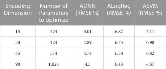
TABLE 6. RMSE(%) and number of optimization parameters for n_opt =17 for different number of encoding dimensions in autoencoder with DNN (ADNN), autoencoder with logistic regression (ALogReg), and autoencoder with SVM (ASVM).

FIGURE 9

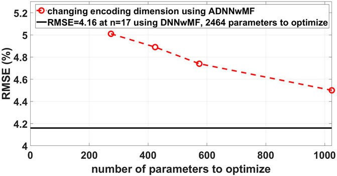
FIGURE 9. RMSE (%) vs. number of optimization parameters.

4 Conclusion

This paper introduces a novel deep learning approach, DNNwMF, to accurately predict the RUL of Li-ion batteries by introducing memory in DNNs. The proposed methodology uses domain knowledge features after capturing the dataset’s trends. The features of current and n previous cycles were used. The paper finds the optimal value of n and shows that introducing memory in this form significantly improves the RUL prediction. Two independent datasets encompassing many testing conditions are used to verify the results. The results are consistent across data sets and test conditions, proving the generalizability of the proposed framework. Furthermore, the results with the proposed framework outperform the classic machine learning approaches like logistic regression and SVM models, establishing the method’s superiority. In addition, ADNNwMF is employed for dimensionality reduction and feature fusion, which considerably reduces the number of optimization parameters. The performance of ADNNwMF improves if the number of encoding dimensions increases. Thus, the proposed methodology is flexible regarding the number of previous cycles and the number of encoding dimensions.

Data availability statement

We used two datasets, one is publicly available at https://data.nasa.gov/dataset/Li-ion-Battery-Aging-Datasets/uj5r-zjdb. Request for availability of CALCE dataset should be emailed to pecht@umd.edu.

Author contributions

MT contributed to the idea, paper drafting, and results generation. The rest of the authors contributed to the concept and review of the paper.

Conflict of interest

The authors declare that the research was conducted in the absence of any commercial or financial relationships that could be construed as a potential conflict of interest.

Publisher’s note

All claims expressed in this article are solely those of the authors and do not necessarily represent those of their affiliated organizations, or those of the publisher, the editors and the reviewers. Any product that may be evaluated in this article, or claim that may be made by its manufacturer, is not guaranteed or endorsed by the publisher.

References

Amir, S., Gulzar, M., Tarar, M. O., Naqvi, I. H., Zaffar, N. A., and Pecht, M. G. (2022). Dynamic equivalent circuit model to estimate state-of-health of lithium-ion batteries. IEEE Access 10, 18279–18288. doi:10.1109/access.2022.3148528

CrossRef Full Text | Google Scholar

An, S. J., Li, J., Daniel, C., Mohanty, D., Nagpure, S., and Wood, D. L. (2016). The state of understanding of the lithium-ion-battery graphite solid electrolyte interphase (sei) and its relationship to formation cycling. Carbon 105, 52–76. doi:10.1016/j.carbon.2016.04.008

CrossRef Full Text | Google Scholar

Deng, Z., Lin, X., Cai, J., and Hu, X. (2022). Battery health estimation with degradation pattern recognition and transfer learning. J. Power Sources 525, 231027. doi:10.1016/j.jpowsour.2022.231027

CrossRef Full Text | Google Scholar

Dong, H., Jin, X., Lou, Y., and Wang, C. (2014). Lithium-ion battery state of health monitoring and remaining useful life prediction based on support vector regression-particle filter. J. Power Sources 271, 114–123. doi:10.1016/j.jpowsour.2014.07.176

CrossRef Full Text | Google Scholar

Gondara, L. (2016). “Medical image denoising using convolutional denoising autoencoders,” in 2016 IEEE 16th International Conference on Data Mining Workshops (ICDMW IEEE), 241–246.

CrossRef Full Text | Google Scholar

Hu, X., Cao, D., and Egardt, B. (2017a). Condition monitoring in advanced battery management systems: Moving horizon estimation using a reduced electrochemical model. IEEE/ASME Trans. Mechatronics 23, 167–178. doi:10.1109/tmech.2017.2675920

CrossRef Full Text | Google Scholar

Hu, X., Xu, L., Lin, X., and Pecht, M. (2020). Battery lifetime prognostics. Joule 4, 310–346. doi:10.1016/j.joule.2019.11.018

CrossRef Full Text | Google Scholar

Hu, X., Zou, C., Zhang, C., and Li, Y. (2017b). Technological developments in batteries: A survey of principal roles, types, and management needs. IEEE Power Energy Mag. 15, 20–31. doi:10.1109/mpe.2017.2708812

CrossRef Full Text | Google Scholar

Jiang, B., Dai, H., Wei, X., and Jiang, Z. (2021). Multi-kernel relevance vector machine with parameter optimization for cycling aging prediction of lithium-ion batteries. IEEE J. Emerg. Sel. Top. Power Electron. 11, 175–186. doi:10.1109/jestpe.2021.3133697

CrossRef Full Text | Google Scholar

Liu, D., Pang, J., Zhou, J., Peng, Y., and Pecht, M. (2013). Prognostics for state of health estimation of lithium-ion batteries based on combination Gaussian process functional regression. Microelectron. Reliab. 53, 832–839. doi:10.1016/j.microrel.2013.03.010

CrossRef Full Text | Google Scholar

Liu, J., Saxena, A., Goebel, K., Saha, B., and Wang, W. (2010). An adaptive recurrent neural network for remaining useful life prediction of lithium-ion batteries. Tech. rep., National Aeronautics and Space Administration Moffett Field Ca Ames Research.

Google Scholar

Meng, J., Stroe, D.-I., Ricco, M., Luo, G., and Teodorescu, R. (2018). A simplified model-based state-of-charge estimation approach for lithium-ion battery with dynamic linear model. IEEE Trans. Industrial Electron. 66, 7717–7727. doi:10.1109/tie.2018.2880668

CrossRef Full Text | Google Scholar

Pinson, M. B., and Bazant, M. Z. (2012). Theory of sei formation in rechargeable batteries: Capacity fade, accelerated aging and lifetime prediction. J. Electrochem. Soc. 160, A243–A250. doi:10.1149/2.044302jes

CrossRef Full Text | Google Scholar

Ren, L., Zhao, L., Hong, S., Zhao, S., Wang, H., and Zhang, L. (2018). Remaining useful life prediction for lithium-ion battery: A deep learning approach. IEEE Access 6, 50587–50598. doi:10.1109/access.2018.2858856

CrossRef Full Text | Google Scholar

Saha, B., and Goebel, K. (2019). Battery data set, nasa ames prognostics data repository; nasa ames. Moffett field, ca, usa.

Google Scholar

Saha, B., Goebel, K., and Christophersen, J. (2009). Comparison of prognostic algorithms for estimating remaining useful life of batteries. Trans. Inst. Meas. Control 31, 293–308. doi:10.1177/0142331208092030

CrossRef Full Text | Google Scholar

Sbarufatti, C., Corbetta, M., Giglio, M., and Cadini, F. (2017). Adaptive prognosis of lithium-ion batteries based on the combination of particle filters and radial basis function neural networks. J. Power Sources 344, 128–140. doi:10.1016/j.jpowsour.2017.01.105

CrossRef Full Text | Google Scholar

Song, Y., Liu, D., Yang, C., and Peng, Y. (2017). Data-driven hybrid remaining useful life estimation approach for spacecraft lithium-ion battery. Microelectron. Reliab. 75, 142–153. doi:10.1016/j.microrel.2017.06.045

CrossRef Full Text | Google Scholar

Stroe, D.-I., Knap, V., Swierczynski, M., Stroe, A.-I., and Teodorescu, R. (2016). Operation of a grid-connected lithium-ion battery energy storage system for primary frequency regulation: A battery lifetime perspective. IEEE Trans. Industry Appl. 53, 430–438. doi:10.1109/tia.2016.2616319

CrossRef Full Text | Google Scholar

Tarar, M. O., Hassan, N. U., and Naqvi, I. H. (2022). “Higher training size, increased model complexity or both: A novel decision framework for cycle life classification of lithium-ion cells,” in 2022 IEEE PES Innovative Smart Grid Technologies-Asia (ISGT Asia) (IEEE), 81–85.

CrossRef Full Text | Google Scholar

Tarar, M. O., Hassan, N. U., and Naqvi, I. H. (2021a). “Modular approach towards battery swapping: Time and technical parameters quality trade-off,” in 2021 IEEE PES Innovative Smart Grid Technologies - Asia (ISGT Asia), 1–5. doi:10.1109/ISGTAsia49270.2021.9715649

CrossRef Full Text | Google Scholar

Tarar, M. O., Hassan, N. U., and Naqvi, I. H. (2021b). “On the economic feasibility of battery swapping model for rapid transport electrification,” in 2021 IEEE PES Innovative Smart Grid Technologies Europe (ISGT Europe), 1–5. doi:10.1109/ISGTEurope52324.2021.9639986

CrossRef Full Text | Google Scholar

Tarar, M. O., Hassan, N. U., Naqvi, I. H., and Pecht, M. (2023). “Techno-economic framework for electric vehicle battery swapping stations,” in IEEE Transactions on Transportation Electrification.

CrossRef Full Text | Google Scholar

Tarar, M. O., and Khalid, Z. (2021). “Reconstruction of finite rate of innovation spherical signals in the presence of noise using deep learning architecture,” in 2020 28th European Signal Processing Conference (EUSIPCO) (IEEE), 1487–1491.

CrossRef Full Text | Google Scholar

Wu, J., Zhang, C., and Chen, Z. (2016). An online method for lithium-ion battery remaining useful life estimation using importance sampling and neural networks. Appl. Energy 173, 134–140. doi:10.1016/j.apenergy.2016.04.057

CrossRef Full Text | Google Scholar

Xing, Y., Ma, E. W., Tsui, K.-L., and Pecht, M. (2013). An ensemble model for predicting the remaining useful performance of lithium-ion batteries. Microelectron. Reliab. 53, 811–820. doi:10.1016/j.microrel.2012.12.003

CrossRef Full Text | Google Scholar

Xiong, R., Tian, J., Mu, H., and Wang, C. (2017). A systematic model-based degradation behavior recognition and health monitoring method for lithium-ion batteries. Appl. Energy 207, 372–383. doi:10.1016/j.apenergy.2017.05.124

CrossRef Full Text | Google Scholar

Xu, L., Deng, Z., Xie, Y., Lin, X., and Hu, X. (2022). A novel hybrid physics-based and data-driven approach for degradation trajectory prediction in li-ion batteries. IEEE Trans. Transp. Electrification, 1. doi:10.1109/tte.2022.3212024

CrossRef Full Text | Google Scholar

Xu, X., and Chen, N. (2017). A state-space-based prognostics model for lithium-ion battery degradation. Reliab. Eng. Syst. Saf. 159, 47–57. doi:10.1016/j.ress.2016.10.026

CrossRef Full Text | Google Scholar

Yuchen, S., Datong, L., Yandong, H., Jinxiang, Y., and Yu, P. (2018). Satellite lithium-ion battery remaining useful life estimation with an iterative updated rvm fused with the kf algorithm. Chin. J. Aeronautics 31, 31–40. doi:10.1016/j.cja.2017.11.010

CrossRef Full Text | Google Scholar

Zhang, Y., Wik, T., Bergström, J., Pecht, M., and Zou, C. (2022). A machine learning-based framework for online prediction of battery ageing trajectory and lifetime using histogram data. J. Power Sources 526, 231110. doi:10.1016/j.jpowsour.2022.231110

CrossRef Full Text | Google Scholar