Optimal storage for solar energy self-sufficiency

1 Introduction

Moving away from fossil fuels to renewable energy is a crucial step to minimize the extent of global warming. Because renewable energy sources, such as wind and solar, are intermittent, achieving a 100% renewable scenario requires either a large excess generation capacity, a substantial amount of storage, or a judicious mixture of the two. Understanding the nature of is tradeoff between excess capacity and storage is crucial for the design and optimization of effective renewable energy systems. Understanding the factors that determine the tradeoff will improve our grasp of the right balance between the uncertain costs of generation and storage in the future.

This tradeoff is characterized by two fundamental parameters: The generation factor g, the ratio of the average annual generation capacity to the annual load, and the storage capacity S, the number of days of electrical load that reside in a storage system. Various simulation studies have given scattered values for the optimal mix of g and S values, with little understanding of how they depend on physical parameters. Shaner et al. (2018) examined combined energy generation and storage systems in the United States and in specific subregions, with both wind and solar generation. For solar-only generation, a system with g ≈ 2.1 and a storage equivalent S of 4 days of load was virtually 100% reliable, defined as the fraction of total energy demand that was met by renewables plus storage. However, equally high reliability was obtained with g ≈ 1.3 and a month of storage. Heide et al. (2010) focused on the case g = 1, with a mix of solar and wind energy and found that a storage S of 1.1–2.5 months was required.

Tong et al. (2020) developed optimized energy systems for the continental United States over a range of storage costs, using the same underlying model as in Shaner et al. (2018). For inexpensive storage, they found g ≃ 2.2, while more expensive storage required an increase in the capacity to g ≃ 2.7. Concomitantly, the amount of storage dropped from about 5 days of load to 1 day. Budischak et al. (2013) determined optimal solutions for a power network in the eastern United States with disparate storage modalities. The requisite g values were in the range of 2.5–2.9 and S between 0.3–3 days, depending on the type of storage. Related studies Heide et al. (2011); Rasmussen et al. (2012); Jacobson et al. (2015); Cebulla et al. (2017) added easily dispatchable renewable sources, such as hydroelectric power, which reduced the required storage.

Given the range of the these predictions about optimal configurations, a need exists for an analytical theory that would: 1) clarify the relation between input physical parameters and the performance of a combined generation/storage system, and 2) help constrain the parameters of this system to guide the realm of feasibility. In this work, we construct such a theory that is based on an idealized, but general model that faithfully incorporates the actual solar irradiation statistics, including seasonality and day-to-day correlations. This theory allows us to specify the nature of an optimal generation/storage system and make explicit predictions about its cost and reliability. Although optimal systems will in general include both wind and solar energy, we treat only solar energy in order to obtain a theoretically tractable model. We believe that the general features of our results will hold for mixed systems as well.

Our model extends previous analytical theories that were based on simplified solar irradiation statistics. Gordon and Zoglin (1986) assumed a deterministic day-night profile, while ignoring daily and seasonal fluctuations. Bucciarelli (1984); Bucciarelli (1986) and Gordon (1987) included daily, but not seasonal weather variations, and day-to-day correlations in some cases. They found that the failure probability decays exponentially with increasing storage capacity, and Gordon (1987) gave explicit formulas for the storage capacity required to achieve a given reliability. Markvart (1996) included the effects of seasonality in generation and/or load but did not treat random weather fluctuations. Egido and Lorenzo (1992) used an empirical fit to reliability simulations based on historical weather data (including seasonality), and found an exponential relationship between generation and storage. However, a principled theory that quantitatively treats the combination of stochastic daily weather fluctuations, day-to-day correlations, and seasonality does not yet seem to exist. Here we develop such a theory.

We begin by first outlining basic features of the solar-flux data for the St. Louis region, which typifies those of the entire United States. We then introduce our data-driven model and use it to develop analytic formulas for the failure rate and storage capacity needed to achieve a given reliability. We use these to calculate the generation and storage capacities of a combined system that minimizes the cost and yet is extremely reliable. We verify our predictions based on simulations of millions of years of synthetic data.

2 Empirical background

2.1 Solar flux data

To illustrate the issues and as a preliminary to develop our model, we first present and analyze data for the solar flux on a 270 km × 270 km region centered on St. Louis over the 40-year period 1980–2019. This region is large enough that its energy needs can be met by covering a small fraction of the total land area with solar panels, but small enough that power transmission across the region is nearly lossless and instantaneous. The solar data, from the MERRA-2 dataset Molod et al. (2015), is in the form of the energy flux for each hour of the day from 1980 to 2019 (see Supplementary Section S2). We determine the daily incident energy per unit area by multiplying each hourly energy flux by the number of seconds in an hour, and then adding these values over a single day. This gives an average daily solar energy per unit area that ranges between roughly 8–25 MJ/m² from the winter minimum to the summer maximum, with daily extrema of 1.53 MJ/m² and 32.1 MJ/m² over the 40 years of data (Figure 1; 2). For simplicity in our analysis, the data for February 29 in leap years are dropped, so that our results are based on the 40-year period 1980–2019 in which all years consist of 365 days.

FIGURE 1

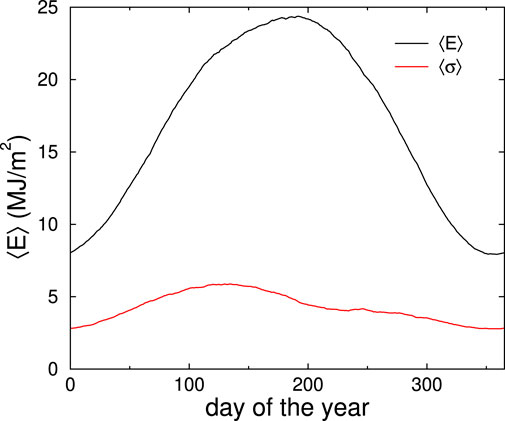
FIGURE 1. Average daily energy ⟨E⟩ per unit area from 1980 to 2019 on the St. Louis region (black), and the daily standard deviation ⟨σ⟩ in this quantity over the same period (red). These data are smoothed by averaging over 45 consecutive days.

FIGURE 2

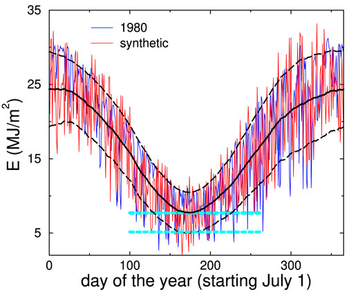
FIGURE 2. Insolation fluctuations. The black curve is smoothed 45-day average daily energy per unit area on the St. Louis region, 1980–2019 and the one standard deviation range is dashed. Also shown is the daily data for 1980 (blue) and a typical realization of our synthetic data (red). The upper dashed blue line corresponds to the load with f = 1 (see text for the definition of f) and the lower corresponds to f = 1.5. The difference between the daily data and the dashed lines gives the daily energy surplus/deficit for these two f values.

The average daily solar energy is roughly sinusoidal, with the maximum at day 189 (July 7, roughly 2 weeks after the summer solstice) and the minimum at day 357 (December 23, a few days after the winter solstice). The standard deviation in the daily solar energy also has a systematic time dependence that ranges between 1.5 and 5.5 MJ/m², with maximal fluctuations occurring in the early spring. Near the winter solstice, the magnitude of the fluctuations is about 35% of the mean value. On the minimum-insolation day, E ≈ 7.95 MJ/m² and σ ≈ 2.79 MJ/m². These numbers, which will play a central role in our ensuing analysis, are based on averaging the daily energy data over a 45-day window.

To illlustrate the influence of fluctuations on the daily insolation data, Figure 2 shows the daily solar flux on the St. Louis region for the single year 1980. For later convenience in our theoretical and numerical modeling, the time origin has been shifted so that the year begins on July 1. The basic feature of these data is that daily solar fluctuations significantly perturb the average annual cycle. Around the winter solstice, which is the most crucial time of the year for the reliability of a combined solar generation and storage system, the minimum solar insolation is roughly a factor 5 less than the average maximum solar insolation. If the storage system is nearly depleted near the winter solstice, multiple overcast days can quickly lead to a system failure. Thus day-to-day fluctuations in solar flux play an important role in determining the optimal tradeoff between generation and storage.

2.2 Generation and storage costs

Our determination of the optimal system configuration is based on two key costs: the cost C_g of the generation capacity to supply the daily electrical energy load L at the winter solstice (based on the average insolation on that day), and the cost C_s of energy storage to cover 1 day of electrical load. This daily load of the St. Louis region is¹ roughly 4 × 10¹⁴  J, or 1.1 KWh × 10⁸ KWh. This corresponds to an average power usage of 4.6  KWh × 10⁶ kW.

It is conventional to express the cost of solar panels in dollar per watt. Using the current solar panel cost of $1.50/W Energysage (2020), the cost of generation is thus C_g ≈ $75 billion. This cost grows roughly linearly with the area of the solar farm². For 20% efficient solar cells (close to the best that are currently available Solar Reviews (2020), the required solar farm area is 4 × 10¹⁴ J/(0.20 J/m² × 7.95 J/m² × 10⁶ J/m²) ≈ 2.5 × 10⁸ m² ≡ A₀. This roughly corresponds to a 16 km × 16 km square. The cost of a solar farm of area fA₀, where f is the normalized generation capacity, will therefore be f C_g. The excess generation capacity, (f − 1)L, is a fundamental metric of the generation system. Using the current price of $1.25/m² AG Web (2019) for rural land in the region, the land cost of the solar farm is approximately $300 million; this is negligible compared to the solar panel costs and will be ignored.

The cost to store 1 day of electrical energy load for the St. Louis region at the current price of $200/KWh is C_s = 1.1 × 10⁸ kWh×$200/kWh ≈ $22 billion Ziegler et al. (2019). It is convenient to measure the capacity S of the storage system in units of the daily electrical energy load in the St. Louis region. We define a storage system of capacity S as one that can supply S days of electrical load to this region. The cost of this storage system therefore is C_sS/L.

Since roughly 60% of a 24-hour period is dark at the winter solstice in the St. Louis region and total electrical energy use is roughly time independent in the winter (US Energy Information Administration (2020a); US Energy Information Administration (2020b)), there is a baseline storage need of 60% of the daily load to cover the energy use when it is dark. If there were no day-to-day fluctuations in the solar flux, this baseline storage, together with the solar energy gathered during the day by a solar farm of area A₀ could fully supply the regional electrical energy needs during a 24-hour period at the solstice, and thus throughout the year.

The existence of insolation fluctuations has several essential consequences. First, the optimal area of the solar farm must be larger than A₀ and the storage capacity must be larger than the 60% of daily energy use that is needed to deal with the regular diurnal fluctuations. Second, we will see that it is impractical to achieve 100% reliability with this combined solar generation and electrical storage system. Thus it is necessary to balance the tradeoff between reliability and cost. Establishing how generation capacity and storage combine to achieve a given reliability, and understanding the tradeoff between reliability and cost, are primary goals of this work. We will find that the optimal cost system configuration is determined by the ratio of storage to generation costs, C_s/C_g. The above numbers give roughly 0.3 for this ratio. Since storage costs are rapidly decreasing Ziegler et al. (2019), we will explore the consequences of potential future storage cost reductions by up to a factor of 7.

3 Synthetic data and simulation methods

Because of the substantial day-to-day fluctuations in the solar flux, the 40 years of available data are too sparse to determine the reliability of a combined solar farm/storage system with statistical significance. To formulate a generally applicable theory, we first construct synthetic daily insolation data that faithfully incorporates the annual trends, the daily fluctuations, and the day-to-day correlations that are present in the solar flux data for the St. Louis region. The simple and direct algorithm that we use to construct these data allows us to readily generate time series for millions of years. From these, we obtain statistically meaningful results about the reliability and cost of a combined solar power generation and storage system.

To construct the synthetic data, we require two additional features beyond the average daily incident energy and its standard deviation: 1) the distribution of energy for each day of the year, and 2) the day-to-day energy correlations. The energy distributions away from the winter solstice are irrelevant when f > 1 because there will be ample solar energy plus stored energy to meet the daily load on any given day that is not near the solstice. It is only near the winter solstice that the daily energy distributions become relevant. However, 40 years of data are too sparse to accurately represent these distributions. To obtain daily energy distribution data of reasonable quality, we aggregate these distributions over symmetric time ranges of 15, 31, and 45 days around the minimum solar-energy day (day 357). These distributions are nearly the same for the three time ranges (Figure 3A); this justifies using a universal shape for the daily energy distribution near the winter solstice. For simplicity, we replace the actual and somewhat triangular-shaped distribution by a uniform distribution whose width is chosen to be the same as that of the data.

FIGURE 3

FIGURE 3. (A) The probability distribution P(E) for the daily energy per unit area over symmetric time intervals around the minimum-energy day (day 357). (B) Probability C(n) that the ratios r_j ≡ E_j/⟨E_j⟩ are all greater than or all less than 1 over n consecutive days. Also shown is the exponential best fit to the data in the range n ≤ 13, C(n) ∝ qⁿ, with q = 0.6157.

There are also day-to-day correlations in the energy flux that reflect the well-known feature that the weather on consecutive days is more likely to be similar than different Bucciarelli (1986). To quantify these correlations, we start with the 40-year sequence of normalized daily energies {r_j ≡ E_j/⟨E_j⟩}, where E_j is the energy per unit area on the jth day of the year and ⟨E_j⟩ is its average, with j ranging³ from 1 to 14,600 (40 × 365). We first determine the length of strings of consecutive days for which the ratios r_j are either all greater than 1 or all less than 1. We then obtain the probability distribution C(n) for the number of consecutive days n where all the r_j are greater than 1 or less than 1.

In the absence of correlations in the daily solar flux, the string length distribution would decay in n as C(n) = (1/2)ⁿ. However, the actual correlations decay as qⁿ, with q ≈ 0.6157 over the range of 1–16 days (Figure 3B). Beyond 16 days, the correlations decay more slowly still. However, the frequency of such long strings of 16 days or longer is roughly once every 6 years. In generating our synthetic data, we ignore these extremely rare events and use the simple exponential decay C(n) ∝ qⁿ for all n.

It is now convenient to shift the time origin so that the year begins on July 1. The solar energy E₁ on July 1 (now day 1) is given by

$E_1=⟨E_1⟩+\sqrt{3}{\sigma }_1\left[\text{rand}\left(-\mathrm{1,1}\right)\right](1)$

where rand(−1, 1) is a uniformly distributed random number between −1 and 1. The factor $\sqrt{3}$ ensures that the standard deviation that arises from the uniform distribution matches that of the actual data, and σ₁ the standard deviation on July 1 (see Figure 1).

To determine the solar energy on successive days j, we define the indicator function I_j for j ≥ 1 as follows: For j = 1 I₁ = 1 − 2Θ[rand(0, 1) − 0.5], where Θ is the Heaviside function. Thus I₁ equals +1 or −1, each with probability 1/2. For j > 1,

$I_j=I_{j-1}\{1-2\mathrm{\Theta }\left[\text{rand}\left(\mathrm{0,1}\right)-q\right]\}.(2)$

Thus I_j, which also takes the values ±1 only, has the same sign as I_j−1 with probability q. For each successive day j > 1, the solar energy E_j is given by

$E_j=⟨E_j⟩+I_j\sqrt{3}{\sigma }_j\left[\text{rand}\left(\mathrm{0,1}\right)\right],(3)$

where σ_j the standard deviation on the jth day of the year. This algorithm results in the deviation of the solar energy from the average on the jth day, E_j − ⟨E_j⟩, having the same sign as E_j−1 − ⟨E_j−1⟩ with probability q.

This persistent random-walk construction Weiss and Rubin (1983); Weiss (1994) ensures that the string length distribution asymptotically decays as qⁿ, as in Figure 3B. The synthetic data accurately mimic both the annual variation, as well as the day-to-day fluctuations of the incident energy, as illustrated by a typical realization of synthetic daily energies in Figure 2.

This approach serves our purposes better than the “Moving-Average” models, “Auto-Regressive” models, or combinations thereof that have often been used to model insolation data Inman et al. (2013). These approaches begin with an uncorrelated random process of a given distribution, and use it a starting point for building correlated sequences of daily insolation values. However, there is no guarantee that the daily insolation values have a physically reasonable distribution. For example, if the input distribution is Gaussian, then the insolation values on some days may be negative because of the tails in the distribution. The present method guarantees a physically reasonable distribution of insolation values. Furthermore, it incorporates the daily variations of the width of the insolation distribution. This is important because it is the width of the distribution around the winter solstice that is crucial for the reliability of the system.

With this computational approach, we generate millions of years of synthetic insolation data over a two-dimensional mesh of thousands of (f, S) values. We start with a full storage system, that is, s = S on July 1. For a given pair (f, S), the stored energy s_j on the jth day of the year is a random variable that changes daily according to

$s_{j+1}=s_j+E_j-L,(4)$

where L is the daily load, subject to the constraint that s_j can never exceed S (Figure 4). Since the model treats only the total energy in a day, it does not include the diurnal variation mentioned in Section 2.2 that will require an additional constant storage requirement of 0.6L.

FIGURE 4

FIGURE 4. Schematic and not to scale dependence of the daily energy minus the load near the winter solstice (blue curve), with three periods of below average insolation (a,c,e) and two above-average periods (b,d). The extent of the energy deficits and surpluses are shown by the blue and red shaded areas. The green curve indicates the instantaneous storage s(t) and the green dotted line indicates full storage.

The time evolution in the model defines a biased random-walk-like process on the interval [0, S], in which the bias corresponds to the difference between the daily insolation and the daily load, and the day-to-day insolation fluctuations correspond to random noise. System failure occurs whenever s_j reaches zero. The failure probability ɛ is defined as the fraction of simulated years for which failure occurs.

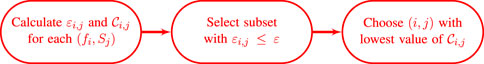
To obtain cost-optimized system configurations within the simulations for a given value of ɛ, we set up a double mesh of the normalized generation capacity values f_i and the storage capacity values S_j. We evaluate the system cost for each mesh point (f_i, S_j) as ${\mathcal{C}}_{i,j}=C_s{S}_i/L+C_g{f}_j$, as well as the failure probability ɛ_i,j. Then we find the pair (i, j) with the lowest ${\mathcal{C}}_{i,j}$ value subject to the constraint that ɛ_i,j ≤ ɛ; f_i and S_j define the optimized system configuration.

4 Generation/storage tradeoff

Due to fluctuations in daily insolation, even a system with f > 1 will be insufficient to supply the electrical load unless storage is included. We will construct a theory to determine the range of possible mixes of generation and storage that achieve a given reliability. We treat only the constraints that arise from storage-capacity limitations and not from power-delivery limitations. We also assume 100% efficient storage, perfect power transmission across the region, and a constant daily load.

The stylized time history of the insolation and stored energy near the winter solstice (Figure 4) also illustrates the tradeoffs involved in optimizing the combined system. In this figure, the energy deficit during period a is larger than the surplus in the following period b. Thus full storage on the jth day is only partially replenished in period b. Conversely, while the storage is fully replenished in period d with a large solar surplus, some of this surplus is wasted because of the limited storage capacity (indicated by the cutoff in the red area). The optimal storage system should maximize the energy returned to storage during surplus days near the winter solstice, while minimizing cost.

4.1 Stored energy distribution

For a solar farm of area A₀, insolation tends to replenish the storage during most of the year; this time range corresponds to what we term the strong-bias regime. Conversely, for an average day near the winter solstice, the insolation roughly matches the load, so that the state of the storage system change only slightly from day to day. We term this time range as the weak-bias regime. In an optimal design, the storage system should be nearly depleted through the winter solstice. Otherwise, excess unused storage capacity exists that increases the system cost without meaningfully increasing its reliability.

For each day of the year, there is a day-specific average distribution of energy in the storage system. We will determine these daily distributions over a period around the winter solstice. From these distributions, we will determine how the annual failure probability ɛ depends on f and S. Section 5 uses these relations to calculate the necessary storage and generation capacity in a cost-optimized system configuration.

To compute the stored energy distribution on a single day, we first treat the idealized situation of a strong and time-independent bias. Based on the biased random-walk picture described above, the distribution of stored energy on the jth day of the year, P_j(s), attains the steady-state form

$P_j\left(s\right)=\mathcal{N}\left(e^{{\lambda }_{j}s}-1\right),(5)$

with normalization constant $\mathcal{N}={\lambda }_j/(e^{{\lambda }_{j}S}-1-{\lambda }_{j}S)\approx {\lambda }_j{e}^{-{\lambda }_{j}S}$ that is determined by requiring that P(s) integrates to 1. A salient feature of Eq. 5 is that the decay constant in the exponential is different for each day of the year. [Related approaches for this distribution were given in Bucciarelli (1984); Bucciarelli (1986); Gordon (1987)].

To begin, we determine the decay constant λ for the case where the bias is fixed. Then we incorporate the effect of a seasonal variation in this bias, as well as the role of day-to-day correlations in the insolation, to find the decay constants in the storage distribution for a range of days about the winter solstice. From these results, we will compute the annual failure probability.

When the bias is constant, the stored energy after each day changes by the average solar energy surplus (or deficit), (f − 1)L, plus or minus a uniform random variable in the range $[-\sqrt{3}f\tilde{\sigma }L,\sqrt{3}f\tilde{\sigma }L]$ to account for day-to-day fluctuations. Here $\tilde{\sigma }=\sigma /E$ is the ratio of the standard deviation in the energy density to the energy density on any given day (see Figure 1). Thus the governing equation for P(s) is

$P\left(s\right)=\frac{1}{2\sqrt{3}f\tilde{\sigma }L}{\int }_{s_{-}}^{s_{+}}P\left(s^{\prime }\right)d{s}^{\prime },(6)$

where $s_{\pm }=s-(f-1)L\pm \sqrt{3}f\tilde{\sigma }L$. This equation is satisfied by the exponential form of Eq. 5, where the decay constant satisfies

$\frac{\sinh \left({\lambda }_{\text{cb}}\sqrt{3}f\tilde{\sigma }L\right)}{{\lambda }_{\text{cb}}\sqrt{3}f\tilde{\sigma }L}=\exp \left[{\lambda }_{\text{cb}}\left(f-1\right)L\right].(7)$

Here we write the decay constant as λ_cb = λ_cb(f), with subscript cb to emphasize that we specialize to the constant-bias case. Eq. 7 gives the dimensionless quantity ${\lambda }_{\text{cb}}L\to 2(f-1)/(f^2{\tilde{\sigma }}^2)$ for f → 1, while λ_cb deviates slightly from linearity for larger f (Supplementary Figure S1 in Supplementary Section S3). Over the practical range of 1 < f < 1.5, this dependence is accurately described by a linear interpolation between λ_cb = 0 at f = 1 and λ_cbL ≈ 5.675 that arises by numerically solving Eq. 7 at f = 1.5. Thus we infer λ_cbL = Γ (f − 1), with Γ ≈ 11.35. As we shall see, this linear interpolation allows us to construct an analytical theory for the failure probability that incorporates both seasonality and fluctuation effects.

Seasonality causes the steady-state distribution of stored energy to be slightly different for each successive day of the year; thus we now write this distribution as P_j(s), with j indexing the individual day. We first determine P_min(s) on the minimum-insolation day, with λ_min the decay rate on this day. This decay rate would equal 0 when f → 1 within the above constant-bias description. However, our simulations show that the storage distribution still has a nearly exponential form even when f = 1 (see Supplementary Section S4). Thus we need to postulate a functional form for the decay constant on the minimum-insolation day that interpolates smoothly between the limiting cases of a value λ₀, which we will determine when f = 1, and Γ(f − 1) when f − 1 is not small. A simple form that satisfies these criteria is

${\lambda }_{\text{min}}\left(f\right)=\frac{1}{2}\left[\mathrm{\Gamma }\left(f-1\right)+\sqrt{(4{\lambda }_0^2+{\mathrm{\Gamma }}^2{\left(f-1\right)}^2}\right].(8)$

We also need the steady-state storage distributions P_j(s) and their associated decay rates λ_j(f) on a range of days around the minimum-insolation day. To obtain these distributions, we use the fact that the average daily generated solar energy E_j on days near the winter solstice is well described by the quadratic $E_j/L=f+f{(j-j_{\text{min}})}^2/{\tau }^2$, where j_min is the day of minimum insolation and τ = 72 (in units of days) is determined by fitting to the 40-year average insolation data. For each day, the effect of the additional bias as one moves away from the minimum-insolation day is equivalent to increasing f by $f(j-j_{\text{min}}^2)/{\tau }^2$. Thus the day-specific decay constant is

${\lambda }_j\left(f\right)={\lambda }_{\text{min}}\left(f\right)+f\mathrm{\Gamma }{\left(j-j_{\text{min}}\right)}^2/{\tau }^2.(9)$

Finally, we need to account for correlations in the daily insolation. To include these effects, we perform stochastic simulations of a system with constant bias f = 1.5 (taken to be typical of the high-f regime) and constant $\tilde{\sigma }=0.351$. Logarithmic plots of P(s) obtained both with and without correlations confirm the exponential behavior of P(s), and show that including correlations reduces the decay parameter by 11%. Thus we take Γ = (0.89) × (11.35/L) = 10.1/L.

4.2 The failure probability

From the distribution of storage for each day of the year, we now determine the annual failure probability ɛ of the storage system. We first estimate the failure probability ɛ_j on each day j, and then add these daily failure probabilities over a time range that includes the winter solstice, to obtain the annual failure probability.

The day-specific failure probability for the jth day of the year in the strong-bias limit is

${\epsilon }_j=\frac{1}{2\sqrt{3}f{\tilde{\sigma }}_{j}L}{\int }_0^{\delta s}{P}_j\left(s\right)\left(\delta s-s\right)ds=A_j{e}^{-{\lambda }_j\left(f\right)S}.(10)$

That is, we integrate the storage distribution P_j(s) over the energy range $\delta s=\sqrt{3}f{\tilde{\sigma }}_{j}L-(f-1)L$, for which for the storage system can be completely depleted within a single low-insolation day, multiplied by the probability $(\delta s-s)/2\sqrt{3}f{\tilde{\sigma }}_{j}L$ that starting with stored energy s, a negative energy step actually depletes the storage system. The expression for A_j is written in the SM and λ_j(f) is the day-specific decay constant in Eq. 9.

To calculate the annual failure probability ɛ, we the sum the daily failure probabilities in Eq. 10 over the range of days where the quadratic dependence of the decay rate in Eq. 9 applies, under the assumption that these daily failure probabilities are all independent. Because of the quadratic time dependence of λ_j(f) in Eq. 9, we convert the sum over a finite range of days j around the insolation minimum to the following Gaussian integral over an infinite time range (see Supplementary Section S5 for details), in which days far from the minimum give negligible contributions:

$\begin{array}{ll}\hfill \epsilon & =\sum _j{\epsilon }_j\simeq {\int }_{-\infty }^{\infty }A\left(t\right)e^{-\lambda \left(t,f\right)S}dt\hfill \\ \hfill & =\frac{B}{\sqrt{{\lambda }_{\text{min}}\left(f\right)S}}{e}^{-{\lambda }_{\text{min}}\left(f\right)S},\hfill \end{array}(11)$

where we replace the index j by the continuous time t, and B is defined in Supplementary Section S5.

We now invert this expression to solve for the required storage as a function of the reliability ɛ. In Supplementary Section S6, we show that the following approximate expression accurately describes the dependence of S on f and ɛ:

$\begin{array}{ll}\hfill S\left(f,\epsilon \right)& =\frac{\ln \left({\epsilon }_0/\epsilon \right)}{{\lambda }_{\text{min}}\left(f\right)}\hfill \\ \hfill & =\frac{2\ln \left({\epsilon }_0/\epsilon \right)}{\left[\mathrm{\Gamma }\left(f-1\right)+\sqrt{(4{\lambda }_0^2+{\mathrm{\Gamma }}^2{\left(f-1\right)}^2}\right]},\hfill \end{array}(12)$

where ɛ₀ is defined in Supplementary Section S6.

Eq. 12 illustrates the two key features of the tradeoff between generation and storage capacities: 1) The storage S depends logarithmically on ɛ; thus a small increase in storage capacity substantially increases the combined system reliability. 2) A small increase in f beyond 1 substantially decreases the required storage capacity (Figure 5).

FIGURE 5

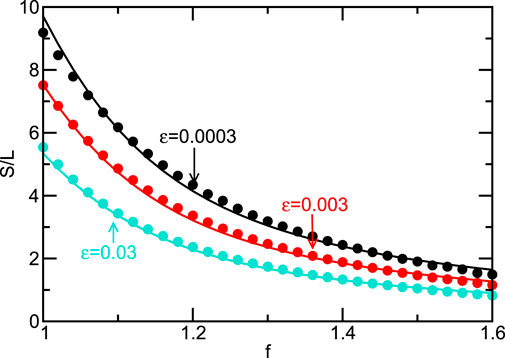
FIGURE 5. Dependence of the storage S needed for a failure probability ɛ, on generation capacity factor f. Circles indicate simulation data and the curves give the theoretical result of Eq. 12. L is the daily load.

5 Cost optimization

We now determine the optimal configuration of the combined system by minimizing the cost function:

$\mathcal{C}=C_s\frac{S\left(f\right)}{L}+C_{g}f.(13)$

Here again C_g = $75 billion is the cost of a solar farm whose area A₀ is just sufficient to supply the daily electrical load L of the St. Louis region during an average insolation day at the winter solstice, while C_s = $22 billion is the cost of a storage system that can supply 1 day of electrical load for the region. As mentioned previously, the cost of the generation system is assumed to be linear in its area, so the cost of a solar farm of area fA₀ will be C_gf. Similarly, a storage system that supplies an energy S will have a cost C_sS/L, under the assumption that the cost of storage is also linear in its capacity.

To find the optimal parameters (f*, S*) in the minimum cost configuration, we set $d\mathcal{C}/df=0$ to give

${\left.\frac{dS\left(f\right)}{df}\right|}_{f^{*},S^{*}}=-L\frac{C_g}{C_s}.(14)$

Thus the optimal system configuration depends only on the ratio of storage to generation cost, C_s/C_g, once ɛ is specified. (The relation between the ratio C_s/C_g and conventional measures of storage and generation costs is given in Supplementary Section S7). The details of this minimization are given in Supplementary Section S8, from which the optimal solar farm size is determined from

$f^{*}=1+\frac{2{\lambda }_0}{\mathrm{\Gamma }}\frac{C_s/\left(C_g{r}_0\right)-1}{\sqrt{2C_s/\left(C_g{r}_0\right)-1}},(15)$

where the dimensionless parameter r₀ is given by

$r_0=\frac{2{\lambda }_0^{2}L}{\mathrm{\Gamma }\ln \left({\epsilon }_0/\epsilon \right)}.(16)$

The optimal storage value S* is then obtained by substituting f* in Eq. 12.

Here, and in what follows, we use ɛ = 0.03 (failure about once every 33 years) because this value roughly corresponds to the accepted standard of a load loss of 1 day per 10 years FERC (2011). For this value of ɛ, r₀ = 0.038. If the cost ratio C_s/C_g, which currently is roughly 0.3, were to become less than 0.038, then Eq. 15 gives f* <1 and indeed f* would not be defined if C_s/C_g became less than 0.019. In this regime, our theory no longer applies, but is also unlikely to be reached by reductions in storage cost in the foreseeable future.

Our theoretical predictions for (f*, S*) agree well with simulation results shown in Figure 6. Over the range of cost ratios shown, S* varies from 1 to 7 days, while f* varies from near 1 to 1.4. To gain insight into the dependences of (f*, S*) on system parameters, it is helpful to focus on the limits of expensive and inexpensive storage.

FIGURE 6

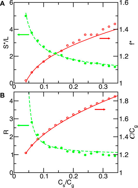
FIGURE 6. (A) Optimal storage value S* and generation capacity f*, as functions of cost ratio C_s/C_g. (B) Ratio R of storage cost to excess generation cost, and the system cost $\mathcal{C}$, as functions of C_s/C_g. In both panels, circles are simulation points, while solid lines are the theoretical predictions of Eqs 12, 15.

5.1 Expensive storage limit

We define this limit as C_s/(C_gr₀) ≫ 1, where (15) reduces to

$f^{*}\simeq 1+\frac{{\lambda }_0}{\mathrm{\Gamma }}\sqrt{\frac{2C_s}{C_g{r}_0}}=1+\sqrt{\frac{\ln \left({\epsilon }_0/\epsilon \right)}{\mathrm{\Gamma }L}\frac{C_s}{C_g}}.(\mathrm{17a})$

When storage is expensive, the combined system favors generation over storage. Consequently, f becomes large, so that we can drop the λ₀ term in Eq. 12 to give

$S^{*}\simeq \frac{\ln \left({\epsilon }_0/\epsilon \right)}{\mathrm{\Gamma }\left(f^{*}-1\right)}=\sqrt{\frac{\ln \left({\epsilon }_0/\epsilon \right)L}{\mathrm{\Gamma }}\frac{C_g}{C_s}}.(\mathrm{17b})$

Thus f* and S* have inverse dependences on the cost ratio C_g/C_s. Combining Eq.17a and Eq. 17b, the ratio R of the total storage cost to the excess generation capacity cost is particularly simple:

$R\equiv \frac{C_s{S}^{*}/L}{C_g\left(f^{*}-1\right)}=1.(18)$

As shown in Figure 6, this ratio is already close to 1 when C_s/C_g exceeds 0.2.

From Eq. 13 to Eq. 18, we may write the total system cost in the equivalent forms

$\begin{array}{ll}\hfill \mathcal{C}& =C_g+2C_s\frac{S^{*}}{L}=C_g+2C_g\left(f^{*}-1\right)\hfill \\ \hfill & =C_g+2\sqrt{\frac{\ln \left({\epsilon }_0/\epsilon \right)C_g{C}_s}{\mathrm{\Gamma }L}}.\hfill \end{array}(19)$

The first term in each of these forms is the “bare” cost of the generation system that would be adequate in the absence of insolation fluctuations. The second term represents the additional system cost that is needed to mitigate the effect of fluctuations. For ɛ = 0.03 and C_s/C_g in the range [0.1,0.3], this additional cost is roughly 50%–80% of C_g or $40–$60 Billion. Eq. 19 also shows that the additional system cost due to fluctuations increases only as $\sqrt{\ln (1/\epsilon )}$. Thus, for example, to reduce ɛ from 0.03 to 0.003, the additional cost needs to be increased by less than 15%.

Eq. 19 also provides an explicit way to decide whether it is more cost effective to invest in reducing the generation cost or the storage cost. The quantity $C_s(\partial \mathcal{C}/\partial C_s)$ gives the sensitivity of the system cost to a given fractional reduction in C_s, while $C_g(\partial \mathcal{C}/\partial C_g)$ plays a similar role for C_g. From Eq. 19, we find

$\frac{C_s\left(\partial \mathcal{C}/\partial C_s\right)}{C_g\left(\partial \mathcal{C}/\partial C_g\right)}=\frac{\sqrt{\ln \left({\epsilon }_0/\epsilon \right)C_s{C}_g/\mathrm{\Gamma }L}}{C_g+\sqrt{\ln \left({\epsilon }_0/\epsilon \right)C_s{C}_g/\mathrm{\Gamma }L}}.(20)$

This cost sensitivity ratio is about 0.3 when C_s/C_g = 0.3. Thus a 30% reduction in storage cost has about the same impact as a 10% reduction in generation cost.

5.2 Inexpensive storage limit

We define this limit by C_s/(C_gr₀) − 1 ≪ 1. Expanding Eq. 15 and the denominator of Eq. 12 to first order in this quantity, we obtain

$f^{*}\simeq 1+\frac{2{\lambda }_0}{\mathrm{\Gamma }}\left(\frac{C_s}{C_g{r}_0}-1\right)=1-\frac{2{\lambda }_0}{\mathrm{\Gamma }}+\frac{\ln \left({\epsilon }_0/\epsilon \right)}{{\lambda }_{0}L}\frac{C_s}{C_g}(\mathrm{21a})$

$S^{*}=\frac{2{\lambda }_{0}L}{\mathrm{\Gamma }}\frac{C_g}{C_s}(\mathrm{21b})$

As C_s/C_g approaches r₀, f* → 1 while S* approaches a constant value, so the excess system cost becomes dominated by the storage cost, as shown in Figure 6.

Combining Eq. 21a and Eq. 21b, the total system cost is now

$\mathcal{C}\simeq C_g+\frac{\ln \left({\epsilon }_0/\epsilon \right)C_s}{{\lambda }_{0}L}.(22)$

For C_s/C_g = 0.04, which is the smallest cost ratio value that we simulated, the additional cost due to weather fluctuations, $(\mathcal{C}-C_g)$, is roughly $\frac{1}{4}{C}_g$. Here, the additional system cost due to fluctuations increases as the logarithm of the inverse failure probability. Thus to reduce ɛ from 0.03 to 0.003 requires a significant increase in the additional cost of about 30%.

The relative influence of cost reductions in storage versus generation is similar to that in the expensive-storage limit. The cost sensitivity ratio now becomes

$\frac{C_s\left(\partial \mathcal{C}/\partial C_s\right)}{C_g\left(\partial \mathcal{C}/\partial C_g\right)}=\frac{\ln \left({\epsilon }_0/\epsilon \right)}{{\lambda }_{0}L}\frac{C_s}{C_g},(23)$

which is about 0.2 at C_s/C_g = 0.04. Thus a 50% reduction in storage cost now has about the same impact as a 10% reduction in generation cost. In both the limits of expensive and inexpensive storage, reducing the generation cost has more impact on the overall cost than reducing storage cost.

6 Discussion

We developed an analytic theory to determine the optimal mix of solar generation and storage that minimizes the overall system cost and achieves a given reliability. This system is specified by f*, the ratio of the solar farm area to the area of a farm that fully supplies the electrical load L for the St. Louis region on the average minimum insolation day, and S* the capacity of the storage system, measured in units of daily load. Our modeling extends the work of Bucciarelli (1984); Bucciarelli (1986) and Gordon (1987) by including seasonal insolation variations, a more realistic distribution of daily energies, and day-to-day correlations in the insolation. Based on a quasi-steady-state approximation for the fill level of the storage system, we obtained the following key results.

• We have shown for the first time that in the presence of seasonal variations, the failure probability decays nearly exponentially with increasing storage and generation capacity (Eq. 11). Previous work that found an exponential decay had ignored seasonal variations Bucciarelli (1984); Bucciarelli (1986); Gordon (1987).

• The storage capacity required to achieve a given reliability (Eq. 12) has a dependence on generation capacity that differs from both the logarithmic dependence found in Gordon (1987) and the exponential one found in Egido and Lorenzo (1992). Without excess generation capacity (f = 1), storage of almost a week of load is required to achieve a failure probability ɛ less than 0.03 (Figure 5). The required storage decreases rapidly when f increases from 1. We also find that the storage need is an increasing function of daily insolation fluctuations, since they reduce Γ in Eq. 12.

• The cost and configuration of the optimal generation/storage system [Eqs. (19), (22), (17a, b), and (21)]. These formulas are the first explicit formulas in the literature for the system cost and configuration in terms of the storage and generation costs.

• A given percent reduction in the generation cost reduces the system cost by three to five times more than the same percent reduction in the storage cost (Eq. 20 and Eq. 23).

A fundamental ingredient in our cost calculations is the ratio of the cost C_g for a solar farm that can supply the daily load of the St. Louis region on an average insolation day at the winter solstice, to the cost C_s of storing 1 day of energy load. With current technology, this cost ratio, C_s/C_g, is roughly 0.3. From Figure 6, the optimal configuration is then given by (f*, S*) ≈ (1.4, 1.3), which implies an overall system cost of 1.4 C_g + 1.3C_s + 0.6C_s ≈ $147 Billion (where the last term incorporates the diurnal storage need), consistent with Tong et al. (2020). As the storage cost decreases, the optimal generation capacity also decreases until the limiting case of (f*, S*) ≈ (1.0, 5), with overall system cost ≈ $91 Billion, is reached after a 7-fold decrease in storage. If storage costs are smaller still, the optimal value f* becomes less than one, a range where our theory is not valid. Below we outline an approach to treat the range f ≲ 1.

A system cost of roughly $100 Billion seems staggering. However, we emphasize that the long-term cost of a solar/storage system is likely cheaper than natural gas power generation. The construction cost for the requisite 5 GW of natural gas generation for the St. Louis region is roughly $4–5 Billion [EIA (2017), Proest (2021)]. Based on prices in the recent past, the fuel cost per year of operation is about $2.5 Billion [Constellation (2020), EIA (2021)]. However, gas prices have increased by a factor of three recently [Trading Economics (2022)]. Thus, assuming a 20-year amortization, the cost of natural gas generation will lie between $55 Billion, based on the average gas price in the previous decade, and $155 Billion, using the current price. The renewable-energy systems modeled here will be cheaper if the gas price is at the upper end of the range. This finding is consistent with that of Tong et al. (2020), while Jacobson et al. (2015) and Jacobson et al. (2022) found renewable systems to be even more cost-effective. Our estimates neglect maintenance costs, but we anticipate that maintenance of solar/storage will be cheaper than that of natural gas because the former has almost no moving parts. The primary impediment to implementing a solar/storage system is its huge upfront capital cost.

Within a 100% renewable system, costs can be reduced by deploying a mix of solar and wind energy Shaner et al. (2018); Heide et al. (2010). Tong et al. (2020) found that such a mix would reduce costs by about 50% relative to solar-only generation. One advantage of solar/wind generation is that the wind is typically stronger when it is overcast, so an energy deficit in one mode of generation would be offset by a surplus in the other.

If one is willing to forgo 100% renewable energy generation, a solar/storage system could be augmented by natural gas “peaker” plants that operate only during solar energy deficit periods near the winter solstice. Because natural gas generation plants are relatively cheap to build (as mentioned above), they are well suited to being run for just a few days of the year. Thus consider a composite system that consists of a solar farm of area fA₀, with f ≲ 1, which is supplemented by a 5 GW natural gas peaker plant.

In the absence of insolation fluctuations, the annual energy deficit for such a solar farm is approximately (see Supplementary Section S9).

$\mathcal{D}=\frac{\sqrt{2}}{\pi }365L{\left(1-f\right)}^{3/2}\approx 164L{\left(1-f\right)}^{3/2}.(24)$

Assuming that the fluctuation contribution to the energy deficit is constant, and using a daily fuel cost of $7 Million (the price over the past decade), the cost of a combined solar/peaker generation plant, amortized over the assumed lifespan of 20 years, is

$\begin{array}{ll}\hfill C& =\frac{1}{20}f{C}_g+\text{\$}7\text{M}\times \left[164L{\left(1-f\right)}^{3/2}+10L\right]\hfill \\ \hfill & \to \text{\$}\left[\alpha f+\beta {\left(1-f\right)}^{3/2}\right]\text{Billion},\hfill \end{array}(25)$

with α = 3.75 and β = 1.15. In the last line, we ignore the contribution that is independent of f. The crucial ingredient is β/α ≈ 0.307, the relative cost of natural gas to solar. With increasing β (increasing gas price), the cost-optimal value of f will increase. However, regardless of how expensive gas becomes, the cost-minimizing system will always have f < 1—in other words, some use of peakers will be cost-effective. The optimal combination of generation, storage, and peakers is a question to be determined by future analyses. Our analytic results for the failure probability and required storage will aid such efforts.

We developed our mathematical methods for the specific case of the climate in the St Louis region. The same approach can be applied to any geographic region. We expect the general aspects of our findings, such as the nearly-exponential dependence of the failure rate on the storage and excess generation capacities Eq. (11), to hold generally. Different geographic regions will then differ primarily via the parameter values, in two ways: 1) Variations in C_s/C_g. Regions at higher latitudes have lower insolation at the winter solstice, which increases C_g since more solar panel area is needed to satisfy the load. The increased generation cost will shift the optimal system toward more storage. 2) Variations in λ₀, Γ, and τ. The variations in Γ are the most straightforward. It will be smaller in regions with large relative insolation fluctuations; since these fluctuations are mainly due to cloud cover, Γ will be smaller in cloudy regions. This will lead to increased storage and excess-generation capacity requirements. Broadly based systematic studies based on the general formalism developed here will further clarify the geographical variation of system configuration and cost.

Data availability statement

Publicly available datasets were analyzed in this study. This data can be found here: https://gmao.gsfc.nasa.gov/reanalysis/MERRA-2/.

Author contributions

This work was performed equally by AEC and SR.

Funding

This work was partly supported by the National Science Foundation, Grants DMR-1910736 and EF-2133863 to SR. We gratefully acknowledge support from Washington University’s International Center for Energy, Environment, and Sustainability (INCEES).

Acknowledgments

SR thanks Dan Shrag for helpful advice and conversations. We gratefully acknowledge support to AEC from Washington University’s International Center for Energy, Environment, and Sustainability.

Conflict of interest

The authors declare that the research was conducted in the absence of any commercial or financial relationships that could be construed as a potential conflict of interest.

Publisher’s note

All claims expressed in this article are solely those of the authors and do not necessarily represent those of their affiliated organizations, or those of the publisher, the editors and the reviewers. Any product that may be evaluated in this article, or claim that may be made by its manufacturer, is not guaranteed or endorsed by the publisher.

Supplementary material

The Supplementary Material for this article can be found online at: https://www.frontiersin.org/articles/10.3389/fenrg.2023.1098418/full#supplementary-material

Footnotes

¹This is obtained from the continental United States yearly electricity consumption of 4 × 10¹² kWh (https://www.statista.com/statistics/201794/us-electricity-consumption-since-1975/), dividing by 365 to get consumption per day and then by 100 (taking the St. Louis region to contain about 1% of the United States population).

²There is little economy of scale for a large solar farm [Renewable Energy World (2015)]. While the cost per solar panel decreases as the number of installed panels increases, there are additional costs associated with transmitting solar power from the farm to end users. These transmission costs largely negate the installation economy of scale; such costs do not exist for rooftop solar panels for household use.

³There is a small error in the correlation function because we drop the data for the 10 leap days.

References

AG Web (2019). Missouri land values up 4%. Available at: https://www.agweb.com/article/missouri-land-values-4.

Google Scholar

Bucciarelli, L. L. (1984). Estimating loss-of-power probabilities of stand-alone photovoltaic solar energy systems. Sol. Energy 32, 205–209. doi:10.1016/s0038-092x(84)80037-7

CrossRef Full Text | Google Scholar

Bucciarelli, L. L. (1986). The effect of day-to-day correlation in solar radiation on the probability of loss-of-power in a stand-alone photovoltaic energy system. Sol. Energy 36, 11–14. doi:10.1016/0038-092x(86)90054-x

CrossRef Full Text | Google Scholar

Budischak, C., Sewell, D., Thomson, H., Mach, L., Veron, D. E., and Kempton, W. (2013). Cost-minimized combinations of wind power, solar power and electrochemical storage, powering the grid up to 99.9% of the time. J. power sources 225, 60–74. doi:10.1016/j.jpowsour.2012.09.054

CrossRef Full Text | Google Scholar

Cebulla, F., Naegler, T., and Pohl, M. (2017). Electrical energy storage in highly renewable European energy systems: Capacity requirements, spatial distribution, and storage dispatch. J. Energy Storage 14, 211–223. doi:10.1016/j.est.2017.10.004

CrossRef Full Text | Google Scholar

Constellation (2020). What is the average cost per therm of natural gas? Available at: https://blog.constellation.com/2020/05/28/natural-gas-cost-per-therm/.

Google Scholar

Egido, M., and Lorenzo, E. (1992). The sizing of stand alone pv-system: A review and a proposed new method. Sol. energy Mater. Sol. cells 26, 51–69. doi:10.1016/0927-0248(92)90125-9

CrossRef Full Text | Google Scholar

EIA (2017). Construction costs for most power plant types have fallen in recent years. Available at: https://www.eia.gov/todayinenergy/detail.php?id=31912.

Google Scholar

EIA (2021). How much coal, natural gas, or petroleum is used to generate a kilowatthour of electricity? Available at: https://www.eia.gov/tools/faqs/faq.php?id=667&t=3.

Google Scholar

Energysage (2020). How much does a solar panel installation cost? Available at: https://news.energysage.com/how-much-does-the-average-solar-panel-installation-cost-in-the-u-s/.

Google Scholar

FERC (2011). United States of America federal energy regulatory commission. Available at: https://www.ferc.gov/sites/default/files/2020-04/E−7.pdf.

Google Scholar

Gordon, J. (1987). Optimal sizing of stand-alone photovoltaic solar power systems. Sol. cells 20, 295–313. doi:10.1016/0379-6787(87)90005-6

CrossRef Full Text | Google Scholar

Gordon, J., and Zoglin, P. (1986). Analytic models for predicting the long-term performance of solar photovoltaic systems. Sol. cells 17, 285–301. doi:10.1016/0379-6787(86)90018-9

CrossRef Full Text | Google Scholar

Heide, D., Greiner, M., Von Bremen, L., and Hoffmann, C. (2011). Reduced storage and balancing needs in a fully renewable European power system with excess wind and solar power generation. Renew. Energy 36, 2515–2523. doi:10.1016/j.renene.2011.02.009

CrossRef Full Text | Google Scholar

Heide, D., Von Bremen, L., Greiner, M., Hoffmann, C., Speckmann, M., and Bofinger, S. (2010). Seasonal optimal mix of wind and solar power in a future, highly renewable Europe. Renew. Energy 35, 2483–2489. doi:10.1016/j.renene.2010.03.012

CrossRef Full Text | Google Scholar

Inman, R. H., Pedro, H. T., and Coimbra, C. F. (2013). Solar forecasting methods for renewable energy integration. Prog. energy Combust. Sci. 39, 535–576. doi:10.1016/j.pecs.2013.06.002

CrossRef Full Text | Google Scholar

Jacobson, M. Z., Delucchi, M. A., Cameron, M. A., and Frew, B. A. (2015). Low-cost solution to the grid reliability problem with 100% penetration of intermittent wind, water, and solar for all purposes. Proc. Natl. Acad. Sci. 112, 15060–15065. doi:10.1073/pnas.1510028112

CrossRef Full Text | Google Scholar

Jacobson, M. Z., von Krauland, A.-K., Coughlin, S. J., Dukas, E., Nelson, A. J., Palmer, F. C., et al. (2022). Low-cost solutions to global warming, air pollution, and energy insecurity for 145 countries. Energy and Environ. Sci. 15, 3343–3359. doi:10.1039/d2ee00722c

CrossRef Full Text | Google Scholar

Markvart, T. (1996). Sizing of hybrid photovoltaic-wind energy systems. Sol. energy 57, 277–281. doi:10.1016/s0038-092x(96)00106-5

CrossRef Full Text | Google Scholar

Molod, A., Takacs, L., Suarez, M., and Bacmeister, J. (2015). Development of the geos-5 atmospheric general circulation model: Evolution from merra to merra2. Geosci. Model. Dev. 8, 1339–1356. doi:10.5194/gmd-8-1339-2015

CrossRef Full Text | Google Scholar

Proest (2021). Power plant construction: How much does it cost? Available at: https://proest.com/construction/cost-estimates/power-plants/.

Google Scholar

Rasmussen, M. G., Andresen, G. B., and Greiner, M. (2012). Storage and balancing synergies in a fully or highly renewable pan-European power system. Energy Policy 51, 642–651. doi:10.1016/j.enpol.2012.09.009

CrossRef Full Text | Google Scholar

Renewable Energy World (2015). Questioning solar energy economies of scale, 2015 edition. Available at: https://www.renewableenergyworld.com/2016/02/22/questioning-solar-energy-economies-of-scale-2015-edition/#gref.

Google Scholar

Shaner, M. R., Davis, S. J., Lewis, N. S., and Caldeira, K. (2018). Geophysical constraints on the reliability of solar and wind power in the United States. Energy and Environ. Sci. 11, 914–925. doi:10.1039/c7ee03029k

CrossRef Full Text | Google Scholar

Solar Reviews (2020). Solar panel efficiency: Most efficient solar panels in 2020. Available at: https://www.solarreviews.com/blog/what-are-the-most-efficient-solar-panels.

Google Scholar

Tong, F., Yuan, M., Lewis, N. S., Davis, S. J., and Caldeira, K. (2020). Effects of deep reductions in energy storage costs on highly reliable wind and solar electricity systems. Iscience 23, 101484. doi:10.1016/j.isci.2020.101484

PubMed Abstract | CrossRef Full Text | Google Scholar

Trading Economics (2022). Trading economics. Available at: https://tradingeconomics.com/commodity/natural-gas.

Google Scholar

US Energy Information Administration (2020a). Today in energy. Available at: https://www.eia.gov/todayinenergy/detail.php?id=42915.

Google Scholar

US Energy Information Administration (2020b). Today in energy. Available at: https://www.eia.gov/todayinenergy/detail.php?id=10211.

Google Scholar

Weiss, G. H. (1994). Aspects and applications of the random walk. Amsterdam, Netherlands: Elsevier Science and Technology.

Google Scholar

Weiss, G. H., and Rubin, R. J. (1983). Random walks: Theory and selected applications. Adv. Chem. Phys. 52, 363–505.

Google Scholar

Ziegler, M. S., Mueller, J. M., Pereira, G. D., Song, J., Ferrara, M., Chiang, Y.-M., et al. (2019). Storage requirements and costs of shaping renewable energy toward grid decarbonization. Joule 3, 2134–2153. doi:10.1016/j.joule.2019.06.012

CrossRef Full Text | Google Scholar