Fuel performance uncertainty quantification and sensitivity analysis in the presence of epistemic and aleatoric sources of uncertainties

1 Introduction

Best Estimate Plus Uncertainty (BEPU) approaches have been a field of ongoing investigation for safety analyses of nuclear reactors (Martin and Petruzzi, 2021). BEPU aims to alleviate the conservatism typically employed by characterizing and consistently propagating input sources of uncertainties to safety outputs of interest in order to provide confidence in the obtained numerical results. Although BEPU approaches have found success in thermal-hydraulic applications, their use in multi-physics calculations is challenging due to the various multi-physics input sources of uncertainties and their interactions (Martin and Petruzzi, 2021). BEPU wider adoption in licensing and safety studies strongly depends on the quality of the characterization of the input sources of uncertainties and on the approaches used to propagate the uncertainties to the outputs of interest (Zhang, 2019). BEPU is thus tightly related to Verification, Validation and Uncertainty Quantification (VVUQ) (Zhang, 2019).

In this context, the Organization for Economic Co-operation and Development/Nuclear Energy Agency (OECD/NEA) Multi-physics Pellet Cladding Mechanical Interaction Validation (MPCMIV) benchmark aims to provide guidance for validation, uncertainty quantification (UQ), and sensitivity analysis (SA) in multi-physics simulations (De Luca et al., 2018). The benchmark consists of modeling two cold ramp tests performed at the Studsvik R2 reactor in 2005. Even though the benchmark focuses on pellet cladding mechanical interaction (PCMI) through the modeling of the cold ramps, the multi-physics aspect arises from the R2 reactor modeling (core and in-pile loop used for the tests) with reactor physics and thermal-hydraulics being involved. The PCMI is considered by Consortium for Advanced Simulation of Light Water Reactors (CASL) as one of the main challenges in nuclear reactor modeling (CASL, 2020) highlighting the need to improve its best estimate prediction and the associated uncertainties. The MPCMIV benchmark includes different modeling and simulation (M&S) tiers from 3D heterogeneous multi-physics models up to single physic fuel performance models of the PCMI during the cold ramps with imposed boundary conditions. Before developing UQ and SA in multi-physics, guidance for single physics fuel performance are needed as there is a lack of consistent treatment of uncertainties in fuel performance.

In the fuel performance UQ and SA literature, various interesting studies have been performed but usually treating either only aleatoric sources of uncertainties or focusing mainly on the sensitivity analysis. In (Bouloré et al., 2012), the METEOR V2 1D fuel performance code is coupled to the URANIE UQ framework for depletion calculations. The uncertainty is propagated to fuel centerline temperature and Sobol indices are computed using artificial neural networks. In (Gamble and Swiler, 2016), a similar depletion study is performed with Bison finite element fuel performance code coupled to the DAKOTA UQ framework. Both correlation-based sensitivity indices (Spearman and Pearson) and Sobol indices using surrogate models are computed. In (Ikonen, 2016) and (Ikonen and Tulkki, 2014) various sensitivity analysis methods are investigated using FRAPCON in depletion calculations. The results indicate that for some quantities such as the fuel centerline temperature, correlation-based methods can be enough. However, for other quantities such as the gap conductance that can exhibit strongly non-linear and discontinuous behaviors more complex methods like Sobol indices or moment-independent approaches are needed. It was also discussed that strong interactions between input uncertainties can arise supporting the need for appropriate sensitivity analysis methods. In (Feria and Herranz, 2019), fuel performance uncertainties are propagated using FRAPCON for two power ramp tests to assess the PCMI predictive capability. The results indicate a strongly conservative prediction of the PCMI at high burnups with the rigid pellet model being the most important input. When the fuel pellet creep is considered, the predictions improved significantly.

From all these studies, it is clear that the input uncertainties characterization and treatment is very important for fuel performance UQ and SA. In (Bouloré, 2019), A. Bouloré explains some of the possible sources of uncertainties in fuel performance as well as the challenge of their consistent characterization and treatment as aleatoric and epistemic in safety analysis studies. Inverse UQ approaches using experimental data and based on surrogate models can be used to better characterize the input uncertainties. Bayesian techniques for inverse UQ were applied for the Bison fission gas release model in (Wu et al., 2018) and for the fuel thermal conductivity and fission gas release models of an idealized fuel performance model in (Robertson et al., 2018). International activities such as the benchmark For Uncertainty Analysis In Modeling For Design, Operation And Safety Analysis Of LWRs (LWR-UAM) (Hou et al., 2019) and the benchmark for Reactivity-Initiated Accident (RIA) (Marchand et al., 2018) highlight the importance of consistent treatment of input uncertainties and provide some guidance for their propagation, to allow a consistent comparison of the results between the participants.

These recent efforts in better characterizing the input sources of uncertainties need to be followed by a consistent treatment of epistemic and aleatoric uncertainties for UQ and SA. This has rarely been addressed in nuclear engineering studies due to the computationally demanding number of calculations. Notable exceptions, where the epistemic and aleatoric uncertainties are separated can be found (Novog et al., 2008; Helton et al., 2011; Pun-Quach et al., 2013). In (Novog et al., 2008), both type of uncertainties were accounted to establish reactor trip setpoints that ensure safety margins. In (Helton et al., 2011), different probability risk assessment and performance assessment studies are discussed. It is emphasized that sensitivity analysis is very important in order to identify the most important epistemic and aleatoric inputs and reduce the computational time necessary for their consistent treatment. In (Pun-Quach et al., 2013), A BEPU approach is proposed and applied to a dryout modeling.

In this work, the MPCMIV single physic fuel performance tier is selected in order to develop an approach for consistent treatment of epistemic and aleatoric uncertainties and investigate their impact on the measured cladding axial elongation and cladding outer diameter during the first cold ramp test. FAST fuel performance code (Geelhood et al., 2021) is used to model the base irradiation of the fuel rodlet, the refabrication and the first cold ramp test. The consistent treatment of both epistemic and aleatoric uncertainties in UQ studies is very important as discussed in (Roy and Oberkampf, 2011) but requires a nested loop approach that can be computationally prohibitive. The efficient computational performance of FAST and the Reactor Dynamics and Fuel Modeling Group (RDFMG) High Performance Computing (HPC) resources are leveraged to develop the methodology for epistemic/aleatoric UQ and SA. In Section 2, the MPCMIV benchmark is presented together with the corresponding FAST fuel performance modeling and the identified uncertain inputs and outputs of interest. In Section 3, the different steps of the UQ and SA methodology are discussed. In Section 4, the methodology is applied to the MPCMIV first cold ramp test and the results are analyzed. Finally, in Section 5, a discussion is carried out based on the outcomes of this work, and in Section 6 a summary and general conclusions are provided.

2 Modeling and simulation

The MPCMIV benchmark and more particularly the first cold ramp test is selected as the example in which the methodology for uncertainty quantification of epistemic and aleatoric sources of uncertainties will be demonstrated.

2.1 MPCMIV benchmark

The MPCMIV benchmark focuses on the modeling two cold ramp tests performed at the Studsvik R2 reactor. Measurements of the cladding axial elongation during the two cold ramp tests and of the cladding outer diameter after the two cold ramp tests are available to be compared with the M&S results. The benchmark is divided into four modeling fidelity tiers.

(1) Novel M&S tools with high fidelity. These tools involve the capability of 3-D heterogeneous modeling of both the reactor and the in-pile loop (e.g., irradiation loop).

(2) Novel M&S tools with simplified boundary conditions. These tools involve the capability of 3-D heterogeneous modeling of the in-pile loop with imposed boundary conditions for the core.

(3) Traditional M&S tools with simplified boundary conditions. These tools involve the capability of a 3D homogenized modeling of the in-pile loop with imposed boundary conditions for the core.

(4) Fuel performance tools only. These tools model use power and thermal-hydraulics boundary conditions to model only the fuel performance phenomena.

Participants are free to choose which tier is more suitable to their computational tools capabilities. In this work, tier four fuel performance model is used. For each tier, the exercises are divided into four computational phases.

(1) Model development phase. The computational domains of single physics are verified and validated for steady state simulations. It aims at selecting the correct codes for each physics area.

(2) Pre-qualification phase. The computational domains for both the pre-irradiation and the first ramp test are evaluated and validated against experimental data. Multi-physics models for steady-state and transient are developed. The accuracy of the M&S predictions are assessed against experimental data.

(3) Blind simulation phase. The second pre-irradiation and cold ramp tests are modelled using the multi-physics modeling. The participants do not have access to the experimental data for comparison. The uncertain inputs are quantified and the predicted best estimate results together with their estimated uncertainties are obtained.

(4) Post-test phase. The same modeling as (3) is asked but the measured quantities are disclosed. Additional sensitivity analyses studies are performed to evaluate and refine the M&S.

This work focuses on the first cold ramp test and thus covers the model development phase and the pre-qualification phase. Uncertainty quantification studies are performed for the first cold ramp instead of the second in order to be able to compare against the experimental data.

The irradiation of a fuel rod is being modeled using FAST (Geelhood et al., 2021). The modeling can be decomposed into three steps: base irradiation and refabrication, pre-ramp test, and the first cold ramp test. The base irradiation consists of an irradiation of three cycles in the Forsmark two reactor (boiling water reactor). Table 1 presents some of the father rod data available in the specifications (De Luca et al., 2018). Figure 1 shows the linear heat rate (LHR) as well as the axial power profile for the three cycles. The numbers on the axis have been removed due to the benchmark being still on-going. The reactor coolant inlet temperature and outlet pressure are 274°C and 70 bars, respectively. Where modeling data were available, they were used and where there were missing data necessary for the fuel performance modeling, the defaults values in FAST were used while some values are obtained from (Geelhood and Luscher, 2015; Hou et al., 2019) such as the re-sintering density which was selected to be 0.9% of the theoretical density. The default value for the power to fast neutron flux conversion factor in FAST was used (0.221x10¹⁷ (n/m²/s)/(W/g of fuel)) and therefore, the fast neutron flux is proportional to the LHR. The plenum length is not known and so was calibrated in order to obtain the total rod free volume and internal pressure after the base irradiation close to the experimental measurements. In FAST, only the fuel rodlet part of the father rod is being modeled for the base irradiation for computational reasons (large number of calculations for the UQ and SA). The plenum length has been scaled down to conserve the fuel to plenum volume ratio. The discrepancies between the father rod at the rodlet location and the fuel rodlet results are minimal (e.g., < 0.5%).

TABLE 1

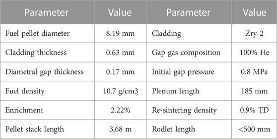
TABLE 1. Father rod and fuel rodlet characteristic.

FIGURE 1

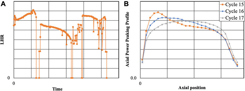
FIGURE 1. (A) Father rod LHR (B) axial relative power for the base irradiation.

After the refabrication, the fuel rodlet has been used to perform a pre-ramp and a cold ramp at the Studsvik R2 reactor. The pre-ramp consists of an irradiation for less than 1 hour at constant power (the fuel rodlet is inserted in the R2 reactor after stabilization at the desired reactor power). Few hours later, the cold ramp was performed. The cold ramp consists of the insertion of the fuel rodlet in the R2 reactor for less than 1 minute with the reactor power being much higher than during the pre-ramp. The reactor is then SCRAM while the rodlet sits in the irradiation facility (in-pile loop 1). The cladding axial elongation was measured during the pre-ramp and the cold ramp test. The cladding outer diameter after the cold ramp was also measured. Therefore, the response of interests selected for the UQ and SA are the maximal cladding axial elongation (elongation obtained right before the SCRAM) and the average cladding outer diameter. Similarly to the base irradiation, the fast neutron flux was determined by FAST using its default power to neutron flux conversation factor value (with the irradiation being very short, it is believed that the fast neutron flux will not have any significant impact during the cold ramp). The axial power distribution was obtained from (Hou et al., 2019). The future neutronic modeling of the Studsvik R2 will help determine the fast neutron flux and the axial power distribution. Figure 2 shows the raw data given in the specification for the LHR and the coolant boundary conditions during the pre-ramp and the cold ramp test. Due to the benchmark being on-going, the data on the axes of Figure 2 have been removed. Figure 2 hence, serves to illustrate the transient conditions qualitatively. The power ramp rate during the cold ramp is between 150 kW/m/min and 180 kW/m/min.

FIGURE 2

FIGURE 2. (A) LHR during the pre-ramp and cold ramp test (B) LHR during the cold ramp only (C) coolant temperature and pressure during the pre-ramp and cold ramp. Due to the benchmark being on-going, the data on the axes have been removed.

2.2 Fuel performance modeling

FAST is the latest U.S. Nuclear Regulatory Commission (NRC) fuel performance code (Geelhood et al., 2021). The version used for this work is FAST-1.0.1 which allows to model steady-state and some transient scenarios for light water reactor mainly. It relies on 1.5D finite difference modeling to solve the heat conduction equation, but also mechanical deformations and fission gas releases. Some other modeling capabilities includes PCMI, cladding creep, ballooning and failure modeling, hydrogen pickup, and oxidation. Some of the limitation of FAST is the implementation of the rigid pellet model: the pellet deformations are due to thermal expansion, swelling, and densification only (fuel creep is not modeled). As many other fuel performance codes, it allows modeling of single fuel rod only.

A fine mesh composed of 90 axial nodes, 30 radial nodes, and 45 radial nodes for the fission gas release was used. The rodlet plenum length is calculated by conservating the fuel length to plenum length ratio of the father rod. The fuel rodlet LHR has been calculated based on the position of the rodlet in the father. The refabrication option was used at half time between the end of the base irradiation and the beginning of the cold ramp test. The fission gas release model used is the Massih model (Geelhood et al., 2021).

2.3 Input uncertainties characterization

As mentioned in the introduction, the characterization and quantification of the input sources of uncertainties is important for any UQ and SA study. The inputs can be classified based on their uncertainty as: aleatoric, epistemic, or a combination of both. Aleatoric uncertainty is an irreducible uncertainty due to inherent stochastic processes that induce variations in the measurement of the quantity. A nuclear engineering example that can be considered as an aleatoric uncertainty is the fabrication process of fuel rod. Epistemic uncertainty is a reducible uncertainty originating from a lack of knowledge. A typical example is the uncertainty of fuel performance models. As highlighted in (Roy and Oberkampf, 2011), due to the difference in their nature epistemic and aleatory uncertainties should not be lumped together in uncertainty propagation studies.

In this work, a total of 30 input uncertainties have been selected. The values for these uncertainties were selected based on the literature (Geelhood et al., 2009; Feria and Herranz, 2019; Hou et al., 2019; Geelhood et al., 2020), while some were based on measurements directly of the R2 reactor. For the aleatoric uncertainties, a normal distribution N(μ, σ) with mean (μ) and standard deviation (σ) was deemed appropriate for this case based on (Geelhood et al., 2009; Feria and Herranz, 2019; Hou et al., 2019; Geelhood et al., 2020). The authors would like to clarify that other distributions can be used if appropriate evidence support them. For the epistemic uncertainties, an interval [a, b] was used following the approach discussed in (Roy and Oberkampf, 2011). The true value of the input/parameter is not known but is believed to be in the interval [a, b], with no value in this interval having a higher likelihood of being the true value (see Discussion section for more details). This lack of knowledge of the true value is mainly due to the impossibility of measuring the input/parameter directly for most cases. Therefore, this treatment of the epistemic uncertainty is addressing the lack of knowledge of the true value rather than considering the input/parameter following an uncertain law. The methodology can be seen as evaluating the effects of the aleatoric uncertainties for multiple plausible values of the epistemic uncertainties. If evidence exists showing a statistical behavior of an epistemic uncertainty, then an associated pdf can be used without changes in the methodology developed. The values for both uncertainty types are shown in Table 2, normalized or centered around 1. The uncertain inputs abbreviation showed in Table 2 will be used throughout the article. FAST allows to directly bias its default material properties and default models parameters for the cladding and the fuel. Therefore, the material properties and/or models parameters depending on some state variable(s) (such as temperature) will retain their dependencies while being biased: a multiplication factor will just be applied to them. The fast neutron flux during both the base irradiation and full ramp test (pre-ramp and cold ramp) was not considered as uncertain due to lack of information. This will be revised once the neutronics results from the benchmark are available. For the characterization of the inputs as epistemic or aleatoric the approach used was to consider as aleatoric the inputs we are more confident about their uncertainty characterization due to the availability of direct measurements while all the others as epistemic. Based on this, boundary conditions, manufacturing parameters and material properties are treated as aleatoric, while model parameters as epistemic.

TABLE 2

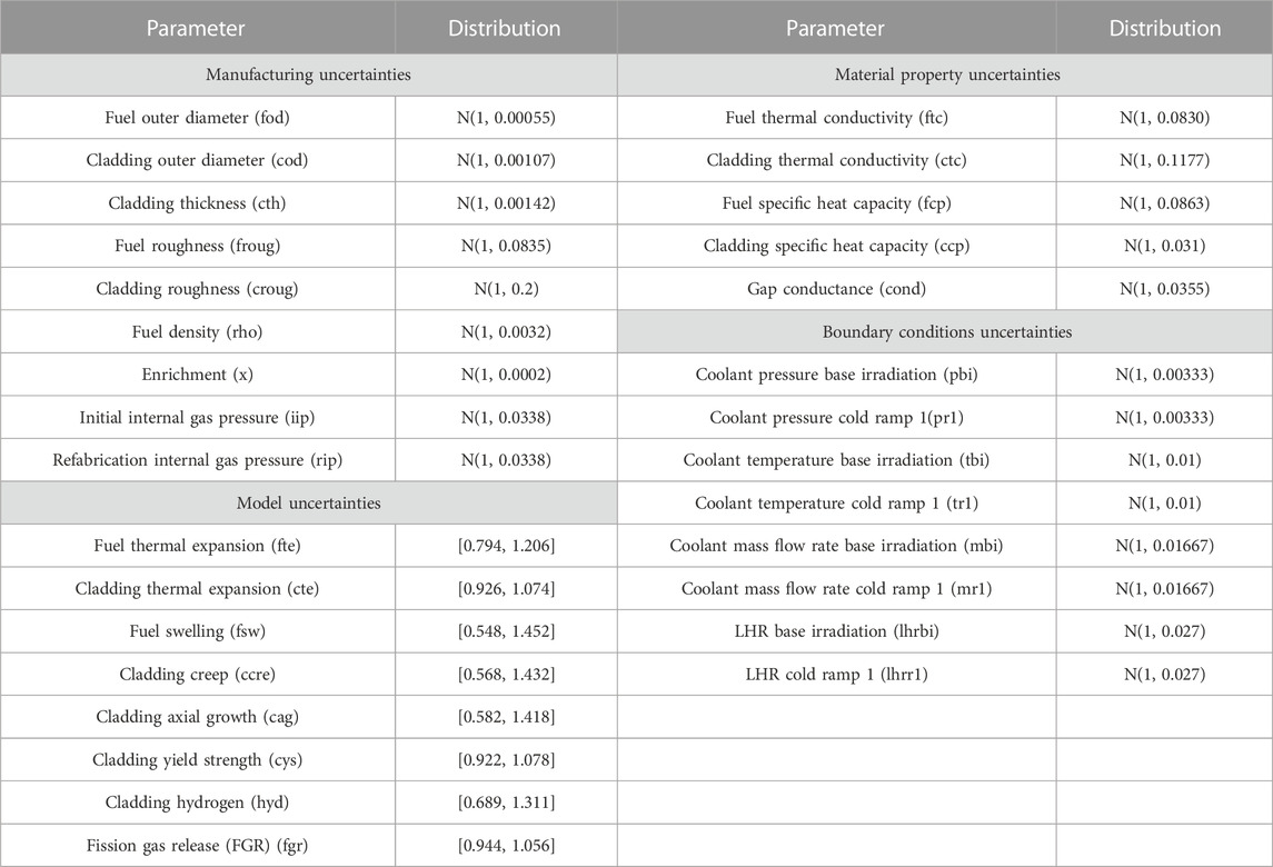
TABLE 2. Uncertain inputs and their respective normalized distributions N(m, s) or [a, b].

3 Uncertainty quantification methodology and theory

3.1 Methodology

The consistent treatment of epistemic and aleatoric uncertainties in fuel performance calculations is very important as discussed in the introduction but can be very computationally demanding. A methodology for fuel performance UQ and SA has been developed and is presented in Figure 3. The methodology leverages the efficient computation capabilities of FAST.

FIGURE 3

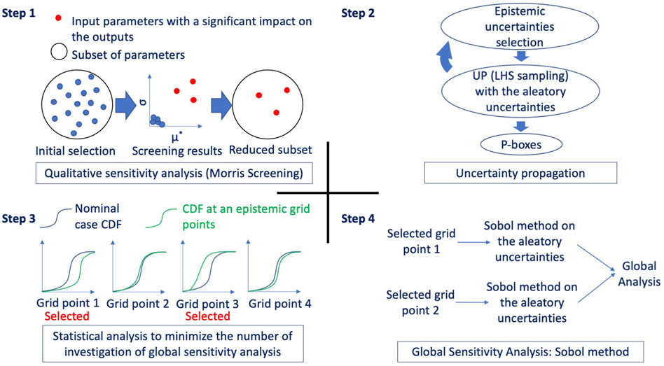
FIGURE 3. UQ and SA methodology.

The first step consists in identifying all possible sources of uncertainties (model, boundary conditions, material properties, manufacturing) and characterizing them based on the available knowledge (experiments, measurements, inverse UQ, indirect evaluations, literature reviews, expert judgment). This was discussed in Section 2.3. Once all the input uncertainties are defined, a qualitative screening analysis is performed using the Morris method to reduce the number of uncertain inputs. This is an important aspect because the nested loop used for the epistemic and aleatoric uncertainty propagation and the sensitivity analysis computational costs depend on the dimension of the effective input space. In this screening, there is no need for separate treatment of epistemic and aleatoric uncertainties. The outcome of this step is a reduced number of inputs that have the largest impact on the output of interest.

The second step of the methodology is the separate propagation of epistemic and aleatoric input uncertainties using a nested loop approach. The epistemic input uncertainties represent a lack of knowledge, something that means that there is a true value for these inputs that lies in the defined interval space, but it is unknown to us. For this reason, in the outer loop, one set of values for the epistemic inputs is selected. In the inner loop, a stochastic sampling is applied to the aleatoric inputs that represents the irreducible uncertainty. The selection of epistemic input values in this work is performed using a full factorial grid of points to ensure that the extremes in this space are covered. If the epistemic input space is high dimensional, sparse grid approaches or stochastic approaches such as Latin Hypercube Sampling (LHS) can be used. The aleatoric uncertainties are sampled using a LHS and the same samples are used for every epistemic grid point. This allows sample to sample comparisons across the various epistemic grid points. Once the nested loop is concluded, the result is a set of aleatoric cumulative density functions (CDF) for every epistemic grid point. The various CDF are combined to construct p-boxes for each output of interest. At this stage some preliminary analysis of the results is carried out by computing correlation-based indices.

The third step involves the selection of critical epistemic grid points where global sensitivity analysis will be performed by computing the Sobol indices. These indices decompose the variance of the output based on the variances of the inputs. Since the epistemic inputs have a true but unknown value, a separate treatment of the epistemic inputs is needed to obtain accurate results, similarly to the UQ (a similar treatment of epistemic and aleatoric uncertainties would potentially leads to epistemic inputs dominating the indices creating misleading results). Therefore, in this methodology we propose to perform Sobol sensitivity analysis only for the aleatoric inputs but for different critical epistemic grid points. This step thus identified these grid points based on a discrepancy metric between the obtained CDFs in the previous step. The metric can be any distance metric between two CDFs and the one used in this work will be detailed in Section 3.3. The critical grid points can then be identified as the epistemic input combinations leading to the highest and/or lowest value of the selected distance metric and thus should reflect the largest variations between the grid points CDFs.

The fourth and last step is the computation of Sobol indices for the selected grid points. As stated above, Ikonen et al. (Ikonen and Tulkki, 2014) showed that interactions between uncertain inputs in fuel performance can be significant and need to be taken into account in sensitivity analysis studies. Sobol indices capture the impact on the output of interest of such interactions, making it therefore a suitable method for fuel performance uncertainty analysis (Sobol’, 1993). However, Sobol indices computations require a large number of calculations. For d uncertain inputs and N samples of at least ${10}^4$, a total of $N\left(d+2\right)\sim {10}^5$ code evaluations are needed (Saltelli, 2002). This can be prohibitive and thus a surrogate model-based approach can be employed to accelerate the calculations. Due to the highly non-linear behavior of PCMI and to the strong interactions between the inputs, surrogate models might not be very accurate for Sobol indices calculations at every grid point. In this work, we perform both direct Sobol indices calculations using FAST and surrogate models. The surrogate models consist of Polynomial Chaos (PC) for every epistemic grid point trained on the samples of the uncertainty propagation step. The accuracy of the PC is assessed on the direct Sobol results.

The surrogate model approach is investigated because in future studies higher fidelity fuel performance codes such as Bison and OFFBEAT could be used that will not afford direct Sobol indices computation (Hales et al., 2016; Scolaro et al., 2020). In this case, a lower fidelity fuel performance code could also be used in the screening step to identify the subset of relevant inputs for the higher fidelity codes.

The following subsections explain the theory behind the different methods employed in the four steps of the methodology.

3.2 Morris screening

Fuel performance has a many uncertain inputs increasing the computational cost of the UQ and SA. To reduce this cost, a screening process, Morris screening method, is performed to reduce the number uncertain inputs. In this method, each uncertain input is discretized over its possible range of value (Morris, 1991). A random combination of all the uncertain inputs is selected and a fixed number of One At a Time (OAT) simulations are performed (OAT: one uncertain parameter is changed at a time while the others are fixed). Then, using another random combination, the same fixed number of OATs are performed. This process is repeated for n(k+1), with n being at least 10 and k being the number of uncertain inputs. At each OAT, the elementary effect of the jth variable (uncertain input) obtained at the ith repetition for a function (here representing the code) $f:X\in {\mathbb{R}}^d\mathbb{⟼}\mathbb{R}$ is:

${E_j}^{\left(i\right)}=\frac{f\left(X^{\left(i\right)}+∆e_j\right)-f\left(X^{\left(i\right)}\right)}{∆}(1)$

With $X^{\left(i\right)}$ the ith combination of input variable $X$, $∆$ being the variation of the jth variable and $e_j$ a vector of the canonical base. Using all the elementary effects, it is possible to determine the mean and standard deviation as seen in Eqs 2, 3, respectively. The mean of the absolute value measures the influence of jth input variable on the output while the standard deviation measures the non-linearity and/or interaction effects of the jth input variable. Therefore, it is possible to distinguish between the uncertain inputs that have neglectable effects on the output, large linear effects without interactions with other uncertain inputs (large ${{\mu }_j}^{*}$), and large non-linear and/or interaction effects (large ${\sigma }_j$). This distinction can be realized visually by plotting the (${{\mu }_j}^{*}$; ${\sigma }_j$) for each uncertain input. The neglectable inputs will be the ones closer to (0, 0). The limit between neglectable and non-neglectable inputs is subjective and is determined by the evaluator.

${{\mu }_j}^{*}=\frac{1}{r}{\displaystyle \sum }_{i=1}^n\left|{E_j}^{\left(i\right)}\right|(2)$

${\sigma }_j=\sqrt{\frac{1}{r}{\displaystyle \sum }_{i=1}^n{\left({E_j}^{\left(i\right)}-\frac{1}{r}{\displaystyle \sum }_{i=1}^n{E_j}^{\left(i\right)}\right)}^2}(3)$

3.3 Uncertainty quantification

Following the Morris screening, a reduced number of uncertain inputs is identified. Each epistemic input is discretized over its possible range of values. Using the discretized space, a full factorial grid of epistemic points is generated. The objective is to perform aleatoric uncertainty propagation (UP) at each grid point. The same aleatoric sampling is used from one grid point to another to allow a higher comparison consistency of the results between each grid point. To perform the UP, many sampling methods exist such as LHS. Using the UP results, the Pearson and Spearman coefficients can be obtained at each epistemic grid point (Hauke and Kossowski, 2011). The Pearson coefficients is a measure of the linear correlation between the input of interest and the output of interest. The possible values range from −1 (fully linear but opposite trends) to 1 (fully linear with the same trend) with a value of 0 meaning no correlation at all. The Spearman coefficients are similar to the Pearson but computed between the ranks of the inputs of interest and outputs of interest. It is a measure of the rank correlation between the input of interest and output of interest, i.e., a value of one means that when the input value increases, the output of interest value increases as well. The Spearman coefficients are therefore between −1 and 1. An analysis of the Pearson and Spearman coefficients at each grid point can provide some information on effects of the aleatoric and epistemic inputs on the output of interests.

At each grid point, a CDF can be constructed for the output of interest. Each CDF depends only on the aleatoric uncertainties, but each CDF is different based on the epistemic combination. Using all the grid point CDFs, it is then possible to build p-boxes (the contour of all the CDFs), see Figure 4. P-boxes represent the minimal and maximal possible distribution for the output of interest. Small p-boxes indicate the low effect of the epistemic uncertainties while large p-boxes show the high impact of the epistemic uncertainties.

FIGURE 4

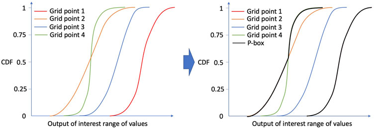
FIGURE 4. UQ results example with p-box.

As mentioned in previous sections, the direct Sobol method requires a high number of computations, making it most of the time not practical to perform on the entire epistemic grid. To alleviate these high computational constraints, an analysis of the CDFs to determine critical grid points is performed. Different metrics can be used to identify critical grid points. In this work, the integral of the surface difference $D_s$ between the CDF obtained for the nominal epistemic grid point (in this paper, it is referred as the reference grid point and reference CDF), denoted by $F_{Nom}:X\in \mathbb{R}\mathbb{⟼}\left[\mathrm{0,1}\right]$, and every other grid point CDF, denoted by $F:X\in \mathbb{R}\mathbb{⟼}\left[\mathrm{0,1}\right]$ is used as defined in Eq. 4.

$D_s=\int \left(F\left(x\right)-F_{Nom}\left(x\right)\right)dx(4)$

The selected grid points are the ones with the highest and lowest $D_s$ values, corresponding thus to the extreme CDFs. These two grid points and the nominal one constitute the three grid points for which Sobol sensitivity analysis is performed. Other distance metrics could be used for specific applications and more grid points could be added if deemed necessary.

3.4 Sobol sensitivity analysis

In fuel performance, the outputs of interest are often functions of non-linearities and interactions between the inputs. Because of that, it is important to use methods that account for these non-linearities and interactions. The Sobol’variance decomposition allows to do so (Sobol’, 1993). Sobol method belongs to the Analysis of Variance (ANOVA) methods that aim to explain the variance of the output based on the variance of the inputs. For a model (here representing the code), noted $f:X\in {\mathbb{R}}^d\mathbb{⟼}\mathbb{R}$, it is possible to decompose it as followed:

$Y=f\left(X\right)=f_0+{\displaystyle \sum }_{i=1}^d{f}_i\left(X_i\right)+{\displaystyle \sum }_{i<j}^d{f}_{ij}\left(X_i,X_j\right)+\dots +f_{12\dots d}\left(X\right)(5)$

With $X$ being the vector of inputs, $Y$ being the output of interest, and $X_i$ being a specific input. For independent inputs, the variance in the output of interest can be expressed as a combination of finite terms, with each term being a function of one or multiple inputs. This decomposition is unique.

$Var\left(Y\right)={\displaystyle \sum }_{i=1}^d{D}_i\left(Y\right)+{\displaystyle \sum }_{i<j}^d{D}_{ij}\left(Y\right)+\dots +D_{12\dots d}\left(Y\right)(6)$

With:

$D_i\left(Y\right)=Var\left(E\left(Y|X_i\right)\right)(7)$

$D_{i,j}\left(Y\right)=Var\left(E\left(Y\left|X_i,X_j\right.\right)\right)-D_i\left(Y\right)-D_j\left(Y\right)(8)$

$D_i\left(Y\right)$ is the variance of $Y$ due to $X_i$ only. In other terms, it is a measure of how much the expected value of Y with only $X_i$ being fixed, varies by changing $X_i$. If the expected value does not change while varying $X_i$, then $D_i\left(Y\right)$ is zero, i.e., the contribution of $X_i$ in the variance of Y is null. Using this definition of the variance, it is possible to define the Solbol’s sensitivity indices which represent the contribution of one input to the total variance of the output of interest, see Eq. 9. For example, for a specific input, the first order sensitivity index, provides how much of the variance of the output of interest can be explained by the contribution of this input only. The second order index is made of the second order interaction of this specific input with another other input (e.g., $X_1{X}_2$_, or $X_1{X}_3$_{,, …)}.

$S_i=\frac{D_i\left(Y\right)}{Var\left(Y\right)},S_{ij}=\frac{D_{ij}\left(Y\right)}{Var\left(Y\right)},\dots (9)$

With:

${\displaystyle \sum }_i{S}_i\le 1(10)$

The first order sensitivity indices require a high number of computations. To obtain higher order indices, even more computations are necessary. Therefore, the total sensitivity indices were introduced to alleviate this burden while obtaining some information on the interaction of the inputs. The total sensitivity index, see Eq. 11, of a specific input is made of the first order sensitivity index plus all its interactions with all the other inputs, i.e., it is a measure of the total effect of the input on the output of interest taking into account all possible interactions with the other inputs. Contrary to the sum of the first order sensitivity indices, the sum of the total sensitivity indices can be above one because the interactions between inputs are counted into multiple total sensitivities indices (e.g., the interaction of $X_1$; $X_2$ is part of $S_{T_1}$; $S_{T_2}$).

$S_{T_i}=\frac{Var\left(Y\right)-Var\left(E\left(Y\left|X_{-i}\right.\right)\right)}{Var\left(Y\right)}=S_i+{\displaystyle \sum }_{j\ne i}{S}_{ij}+{\displaystyle \sum }_{j,k\ne i}{S}_{ijk}+\dots (11)$

With $Var\left(E\left(Y|X_{-i}\right)\right)$ being the total contribution to the variance from non-$X_i$ (defined as fixing all the variables except $X_i$). To obtain the first and total sensitivity indices, Saltelli determined that n(k+2) computation can be used (n being at least 10,000 and k being the number of uncertain inputs) (Saltelli, 2002). n is generally picked to be a power of 2. By obtaining the Sobol sensitivity indices, it is possible to explain quantitatively the behavior of the output of interest based on the input’s uncertainties, allowing a deeper and more detailed understanding of the physics behind the phenomenon modeled.

Although Sobol indices are very informative, they are also very computationally demanding and that is why in most of studies, surrogate models are used for their estimation. Multiple surrogate models exist such as PC and artificial neural networks (Marrel et al., 2008; Cresaux et al., 2009; Bouloré et al., 2012; Gamble and Swiler, 2016). The main advantage of the surrogate model is its low computational time. However, because it is a surrogate model, it models a link between the inputs and the output of interest. Therefore, it is of primary importance to determine the accuracy of the surrogate model. Two processes can be realized to gain confidence in the surrogate model: (1) to compare the results of the code and the surrogate model on a different set of inputs than the ones used to train the surrogate model (Q² value), (2) to compare the sensitivity indices obtained using the Sobol method with direct code evaluations and obtained using the surrogate model. By doing so, one can gain confidence in the surrogate model and use it to estimate all sensitivity indices over the entire epistemic grid. It is however important to remember that the surrogate model can only predict, with some confidence, the sensitivity indices at each point of the epistemic grid and not necessarily on the entire epistemic space at once.

4 Uncertainty quantification results

4.1 Morris screening

The Morris results are presented in Figure 5 for the maximal cladding axial elongation during the first cold ramp test and the average cladding outer diameter after the cold ramp 1. For readability reasons, only the relevant inputs have been identified in Figure 5. The selection of the cut-off limit is generally empirical. Since this paper is focusing on methodology itself, a cut-off limit set at 0.5 of the maxima of the ${{\mu }_j}^{*}$ and ${\sigma }_j$ for each output was selected. The reason for such a high cut-off threshold is to limit the number of uncertain inputs for computational reasons. In our specific case, the addition of the cladding thickness uncertainty would increase the total cost by more than 10% for the Sobol method. Based on these results, in Table 3 the selected inputs that will be used for the UQ and SA are listed.

FIGURE 5

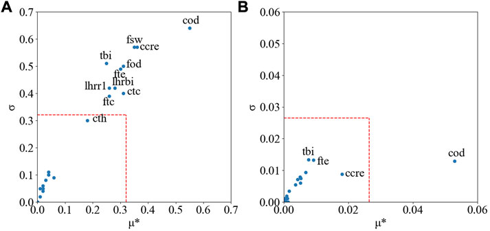
FIGURE 5. (A) Morris results for the maximal cladding axial elongation (B) Morris results for the average cladding outer diameter after the cold ramp. The dash lines represent the cut-off limits.

TABLE 3

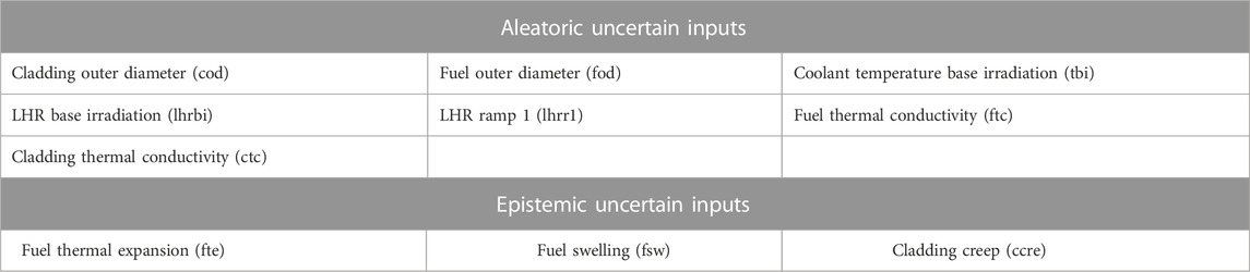
TABLE 3. Reduced uncertain inputs subset.

4.2 Uncertainty propagation and analysis

Each of the three epistemic uncertain inputs were discretized with a total of five values spaced evenly over the entire respective input ranges. We denote $u_i$, the distance between each discrete point for the epistemic input $i$. The inputs ranges being centered on the FAST default value of each model, we have adopted the following notation for describing the discretized values: −2 $u_i$, −1 $u_i$, 0 $u_i$, 1 $u_i$, or 2 $u_i$. Therefore, for an interval [a, b] centered in 1 after normalization, we have a = 1-2 $u_i$ and b = 1 + 2 $u_i$. Hence, the full factorial epistemic grid is composed of 5 × 5×5 (e.g., 125) points. For readiness reasons, the grid points will be denoted only by the coefficient in front of $u_i$: (−2, 1, 0) correspond to (−2 $u_1,1u_2,0u_3)$. Concerning the aleatoric uncertain inputs, the same LHS made of 200 sampling was used at each grid point. The reference grid point and reference CDF are the grid point with no variation of the epistemic uncertain inputs (i.e., the point (0, 0, 0)) and the CDF obtained at this grid point, respectively. Figure 6A shows the reference CDF as well as the p-box for the maximal cladding axial elongation. The values have been normalized using the measurement value (i.e., a value of one means the code predicted the measurement value, the same process was applied for the average cladding outer diameter shown below). From Figure 6 it can be observed that the range of possible values for the axial elongation varies significantly with the epistemic combinations and the aleatoric variations. Only 87% of the grid points results in at least one aleatoric combination leading to a maximal cladding axial elongation of one or above. The difference in shape between the p-box left bound and the right bound, or between the reference CDF below 0.8 and after 0.8, is due to the gap closure happening in the latter case. When gap closure does not happen, the cladding axial elongation is mostly due to the cladding thermal expansion. Meanwhile when gap closure happens, some of the fuel axial elongation is being transmitted to the cladding resulting in a much higher cladding axial elongation.

FIGURE 6

FIGURE 6. Maximal cladding elongation during the cold ramp 1 (A) P-box and reference CDF (B) 5^th, 50^th, and 95^th percentile CDF.

The CDFs for ${\alpha }_{0.05}=0.05$, ${\alpha }_{0.5}=0.5$, and ${\alpha }_{0.95}=0.95$ (i.e., 5^th, 50^th, and 95^th percentile) have been computed and are presented in Figure 6B. A ${\alpha }_y$ cut is obtained by fixing the CDF to a certain value y and looking at the corresponding relative maximal cladding axial elongations for each grid point. ${\alpha }_{0.05}$ covers a very small range while the ${\alpha }_{0.95}$ covers most of the possible values of maximal cladding axial elongation. ${\alpha }_{0.5}$ CDF shows that for many grid points only a few epistemic combinations results in a value of one or above.

Concerning the average cladding outer diameter, Figure 7 shows the reference CDF with the p-box and the $\alpha$ cuts CDFs. The epistemic uncertain inputs seem to shift the CDF more than actually modifying their shape. This is partially due to the lack of plastic deformation on the rodlet. However, when plastic deformation happens, they are very local and so by averaging the diameter over the entire rodlet, their impacts are significantly reduced. Therefore, the impact of the epistemic uncertainties and aleatoric uncertainties are mostly during the base irradiation with a small to none impact on the cladding outer diameter during the cold ramp. Similarly, to the maximal cladding axial elongation, only a few aleatoric combinations for each grid point result in a value equal or above 1. However, in this case, all the grid points have at least one aleatoric combinations resulting in a value equal or above 1. Figures 6, 7 demonstrate the need for a consistent treatment of uncertainty, but also highlight the necessity of more analysis to be able to understand in much deeper details the phenomenon happening.

FIGURE 7

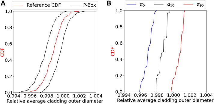
FIGURE 7. Average cladding outer diameter after the cold ramp 1 (A) P-box and reference CDF (B) 5^th, 50^th, and 95^th percentile CDF.

Figures 8, 9 shows the Pearson and Spearman coefficient distributions. The mean corresponds to the average value obtained across the entire full factorial epistemic grid, while the range goes from the minimal to the maximal coefficient values. For the maximal axial cladding elongation, the cladding thermal conductivity seems to have an almost negative linear effect on the maximal axial elongation. A value close to −1 (Pearson and Spearman) is observed for grid points where almost no gap closure is predicted. In this case, the cladding axial elongation is mostly due to the cladding thermal conductivity. As gap closure happens more frequently in the epistemic grid points, the coefficients increase to reach a maximal value of −0.39 indicating that more inputs become influential on the cladding axial elongation. When gap closure happens, the fuel axial elongation is transmitted to the cladding. Gap closure is a complex phenomenon involving possible interaction between uncertain input parameters influencing the fuel temperature (e.g., LHR, fuel conductivity) and/or uncertain input parameters influencing the gap width before the ramp (e.g., fuel and cladding initial diameter). For example, a higher fuel thermal conductivity and lower LHR will have a higher impact on the gap and its closure than the opposite (lower fuel thermal conductivity and higher LHR). Additionally, changing the fuel or cladding outer diameter initial values impacts the gap size initially. This impact is then propagated through the base irradiation. Therefore, if any or both diameters’ uncertainties lead to a smaller gap size, this will be observed as well before the cold ramp. This smaller gap size would then lead to gap closure earlier. Possible interactions with the LHR and the conductivities are therefore possible. The Sobol method will confirm or not the presence of interaction between uncertain inputs. Concerning the average cladding outer diameter, the initial cladding outer diameter has a linear effect on the output as expected. Based on the Pearson and Spearman coefficients for the cladding thermal conductivity, its impact on the average cladding outer diameter seems to be complex (both coefficients can be positive or negative indicating opposing trends). This example shows some of the limitations of the Pearson and Spearman coefficients since the input interactions effects cannot be measured.

FIGURE 8

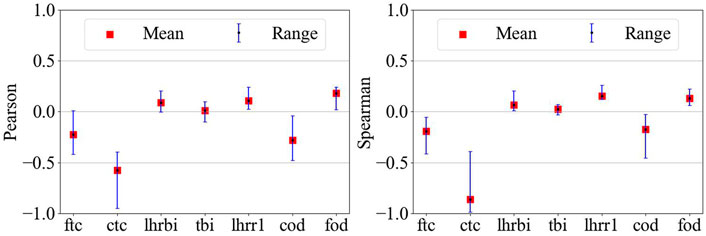
FIGURE 8. Pearson and Spearman coefficient for the maximal cladding axial elongation.

FIGURE 9

FIGURE 9. Pearson and Spearman for the average cladding outer diameter.

The LHR uncertainty during the base irradiation was not considered time dependent and thus did not conserve the burnup for every sample. To determine the impact of this assumption, a time dependent LHR uncertainty was investigated. The base irradiation being divided into three cycles, the first two cycles LHR were applied an independent uncertainty each. Then, using the conservation of the burnup, the LHR of the third cycle was modified accordingly. The UQ results show minimal effects of this new approach.

Using Eq. 4, the following grid points have been selected for the Sobol SA in the next step. The grid points are denoted as the variations of the fuel thermal expansion, fuel swelling, and the cladding creep based on the discretization notation mention above: −2 $u_i$, −1 $u_i$, 0 $u_i$, 1 $u_i$, and 2 $u_i$ with 0 $u_i$ being FAST default value, and ±2 $u_i$ corresponding the interval bounds. For example, the notation (1, 0, 2) would corresponds to one variation of the fuel thermal expansion, 0 variation for the fuel swelling, and two variations of the cladding creep:

- (-2, −2, 0): CDF with the largest area with the reference CDF on its left, i.e., smallest negative metric value, for the maximal cladding axial elongation.

- (2, 2, 2): CDF with the largest area with the reference CDF on its right, i.e., largest positive metric value, for the maximal cladding axial elongation.

- (-2, −2, 2): CDF with the largest area with the reference CDF on its left, i.e., smallest negative metric value, for the average cladding outer diameter.

- (2, 2, −2): CDF with the largest area with the reference CDF on its right, i.e., largest positive metric value, for the maximal outer diameter.

Interestingly, the smallest negative metric value for the maximal cladding axial elongation is not the grid point (−2, −2, −2). The difference in area between the point (−2, −2, 0) and (−2, −2, −2) is only 0.3%. Within that percentage difference lies four other grid points. The reason behind all these results being so close, and therefore showing the relatively small difference between each of these grid point CDFs, is that gap closure almost never happens for most of the aleatoric combinations. Hence, the maximal cladding axial elongation is due only to the cladding thermal expansion and so to the cladding temperature. The reference grid point is added to the list of the selected point for the Sobol SA creating a total of five grid points for the two outputs of interest.

4.3 Sobol sensitivity analysis

The Sobol first order and total indices were computed at each of the selected grid points using FAST. As aforementioned, Saltelli determined that (n(k+2) computation can be used for computing the Sobol indices (n being at least 10,000 and k being the number of uncertain inputs) (Saltelli, 2002). Therefore, a total of 147,456 (=16,384*(7 + 2) = 2¹⁴*(7 + 2)) samples were used. Figures 10, 11 show the results for the maximal cladding axial elongation and the average cladding outer diameter, respectively. S1 is for the first Sobol index while ST is for the total Sobol index. For the maximal cladding axial elongation, it can be observed that for the grid point with low amount of gap closure (i.e., −2,-2,0), the cladding thermal conductivity has a total index of 0.8 and a first index of 0.59. As mentioned above, the cladding axial elongation is mostly due to the thermal expansion of the cladding and therefore, the conductivity of the cladding impacting the temperature has a strong impact. However, as more and more gap closure is observed in the grid points, the contribution of the fuel thermal conductivity and initial cladding outer diameter indices increase as the cladding thermal conductivity decreases. A lot of interaction can be observed especially for the grid point (2,2,2) (grid point with the highest metric for the cladding axial elongation). These three inputs are the ones that influence the most the gap width during the cold ramp. Interaction between them leads to gap closure sooner or later and on a higher proportion of the rodlet. Therefore, they determine how much of the fuel axial elongation is being transmitted to the cladding. Concerning the average cladding outer diameter, it is mostly influenced by the initial cladding outer diameter due to the lower impact of the local plastic deformations with the averaging. The grid point (2,2,2) (not part of the grid points selected in the prior step for the average cladding outer diameter) was added to Figure 11 because of the different trend observed. At the grid point (2,2,2), a lot of plastic deformation appeared, therefore impacting the cladding diameter. This is translated by the lower initial cladding outer diameter indices and the slight increase in the cladding and fuel thermal conductivity which impact the gap closure and also the fuel thermal expansion, therefore the plastic deformation of the cladding.

FIGURE 10

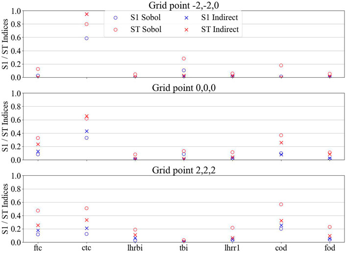
FIGURE 10. First (S1) and total (ST) Sobol indices for the maximal cladding axial elongation. Sobol means indices were calculated from the Sobol method while indirect means from the surrogate model.

FIGURE 11

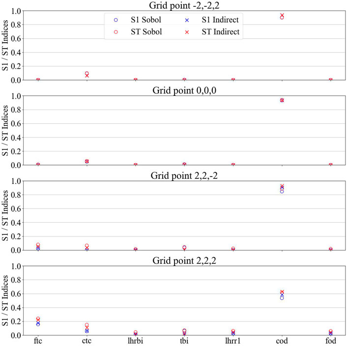
FIGURE 11. First (S1) and total (ST) Sobol indices for the average cladding outer diameter. Sobol means indices were calculated from the Sobol method while indirect means from the surrogate model.

From Figure 10, it can be deduced that the uncertainties on the cladding outer diameter and fuel outer diameter only have significant impact when gap closure happens: both uncertainties impact the gap size before the cold ramp. Based on the Sobol results, it seems the cladding thickness might have some none-negligible impact in some cases since it impacts the gap size as well. However, during the Morris screening results analysis, the cladding thickness was not selected has an important uncertain parameter. The uncertainty on the cladding thickness has a standard deviation 40% larger than the cladding outer diameter (and almost three times larger than the fuel cladding outer diameter), but the cladding thickness is many times smaller than fuel and cladding outer diameters. Therefore, the uncertainty on the cladding thickness has a much smaller impact on the gap size than both uncertainties on the diameters: varying each of these parameters by one of their respective standard deviations, the cladding thickness would lead to a decrease of 1.1% of the gap size, the fuel outer diameter to 2.6%, and the cladding outer diameter to 6.1%. Looking at the Sobol results, it is therefore possible to conclude that the cladding thickness would have a none significant impact on the maximal cladding axial elongation and cladding outer diameter because it impacts on the gap size being much smaller than the diameters uncertainties.

For each grid point where the Sobol indices were computed, the PCs were trained on the same grid point using the results from the UP step. Second order polynomials are used leading to interaction in X_IX_J only. The results obtained are shown in Figures 10, 11 with the notation “Indirect”. It can be observed that the surrogate model accuracy for the average cladding outer diameter is relatively high. The minimal R² value for the five grid points is 0.99. Concerning the maximal cladding axial elongation, accuracy is lower with some grid points being more inaccurate than other (e.g., grid point (0, 0, 0) vs. (−2, −2, 0)). The R²values vary from 0.946 to 0.994. Q² values were computed using the SA sampling and outputs. The values for the maximal cladding axial elongation varies between 0.905 and 0.974, with the lower values being for the grid points with the highest discrepancies in the Sobol indices. For the average cladding outer diameter, the values are above 0.99.

The average cladding outer diameter variance seems to be mostly explained by the initial cladding outer diameter in an almost linear relationship. In this case, almost no input interactions are observed, and the PCs are able to capture that very effectively. This demonstrate the correct implementation of the surrogate model. In a much more complicated case, such as for the maximal cladding axial elongation, interactions between inputs are observed and do not seem to be captured by the PCs in two grid points ((-2,-2,0) and (2,2,2)). The reasons behind these poor performances are being investigated.

5 Discussion

An important part of the methodology relies on the judgment of the evaluator concerning if an uncertainty is epistemic or aleatoric. Some uncertainties are well characterized by experiments directly on the rod being modeled, however in many cases it is not true. Uncertainties obtained from the literature, as it is the case in this paper, are treated as aleatory or epistemic depending on the evaluator estimates that they relate to its case. Therefore, two evaluators would not necessarily have the same epistemic uncertain inputs space for the same modeling. Unfortunately, there is no method to really determine if an uncertain input should be considered epistemic or not. Another problem might arise when too many epistemic uncertainties are present, and the computational cost is too expensive to treat them accordingly. This will need to be addressed in the future especially when multi-physics UQ and SA will be performed.

The treatment of epistemic uncertainties in this paper is realized by using an interval of possible values with no probability attached. Other methods could be used as well, such as Fuzzy theory (Hanss and Turrin, 2010; He et al., 2015). It is also possible to treat the uncertainties as a combination of epistemic and aleatoric. For example, the input can be associated with a normal distribution with an uncertain standard deviation and mean. Such treatment might require more information on the uncertain inputs but would allow a more accurate modeling of the uncertainties. Normal distributions and intervals for both types of uncertainties are used in this paper. However, as aforementioned, other probability treatments can be used. The selection of a probability law should be evidence based, if possible. The methodology proposed here is agnostic to the selected input uncertainty quantification.

The methodology presented in this paper can be used in combination with a low-fidelity code as a screening for a much more computationally expensive high-fidelity code. The conclusions of the low-fidelity code SA are used to determine the uncertain inputs and grid points of importance for the scenario being modeled. More analysis can then be performed with higher fidelity codes.

The objective of the presented methodology is to understand better the physical phenomena involved and to treat uncertainties consistently in terms of their fundamental nature. The separation thus of epistemic and aleatoric uncertainties can be considered as a more accurate approach similar to how using a 3D finite elements code is more consistent in terms of modeling approximation than a 1.5D finite difference code. Considering epistemic uncertainty as interval, as done in this work, can leads to a wide range of values for the any percentile of all CDFs rather than a single value. Figure 12 shows the results of the uncertainty propagation in the case all uncertain inputs are treated as aleatoric. The p-boxes previously obtained are also shown. It can be observed that using only aleatoric uncertainties yields a single curve inside the p-boxes previously obtained. In BEPU, the 95^th percentile value (and/or 5^th percentile value) is generally investigated for safety concern. The authors would like to call this approach the horizontal analysis: a percentile is selected, and a horizontal line can be drawn at this value for analysis (see Figure 12 and the 95^th percentile). To have a more complete analysis regarding safety concerns, the authors thinks that performing a vertical analysis is also necessary. For example, for the relative maximal cladding axial elongation, the 95^th percentile lies within the [0.36, 1.56] interval. Using only aleatoric, the 95^th percentile value is 1.1. A vertical analysis for the relative maximal cladding axial elongation of 1.4 gives that only 15% of the epistemic grid point leads to this value being reached with for a percentile between the 90^th and the 95^th percentiles, and only 7^% with a percentile between the 80^th and the 90^th percentiles. The lowest percentile value being the 80^th percentile. This vertical analysis provides a more complete analysis for safety concerns.

FIGURE 12

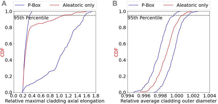
FIGURE 12. UQ results considering all uncertainties as aleatoric for the (A) relative maximal cladding axial elongation and (B) relative average cladding outer diameter. P-boxes obtained previously are also shown for comparison.

In BEPU, the input’s uncertainties are propagated to a safety output of interest and then statistical metrics are computed that could be compared to safety limits. As explained in the above paragraph, the methodology leads to different results compared to traditional methodology, but the results obtained can still be used for safety limit with a different analysis as shown above. Therefore, the authors think the developed methodology can be suited for BEPU, but it increases the computational cost requiring a careful consideration of its usage in a similar way to how 3D finite elements are used. An example commonly used is the estimation of the 95^th percentile with 95% confidence using the Wilk’s formula (Wilks, 1941). Using the Wilk’s formula for the 95^th percentile with 95% confidence and considering all inputs as aleatoric, the upper value found is 1.58 for the relative maximal cladding axial elongation. This value is actually larger, and therefore more conservative, than the upper bound of the 95^th percentile determined using the methodology developed (i.e. 1.56). However, it is not possible make a general conclusion regarding if the developed methodology is more conservative than Wilk’s formula. It is important to note that using the Wilk’s methodology implies that all uncertain inputs are treated the same (no separation of epistemic and aleatoric uncertainties). A more accurate process would be to perform the Wilk’s methodology for the aleatoric uncertainties only but at different epistemic grid point. For the reference grid point, Wilk’s formula would lead to a 95^th percentile with 95% confidence of 1.33. Another analysis of the results obtained and not possible with Wilk’s, for example, would be to estimate the contribution of the aleatoric uncertainties and epistemic uncertainties to the maximal value of 95^th percentile, see Eq. 12. A simple way of doing is to take the average value; ${\mathrm{M}\mathrm{e}\mathrm{a}\mathrm{n}}_{\mathrm{R}\mathrm{e}\mathrm{f}\mathrm{e}\mathrm{r}\mathrm{e}\mathrm{n}\mathrm{c}\mathrm{e}}$, obtained (0.29 for at the reference grid point). Then, the aleatoric uncertainties would lead to the vertical variations up to the 95^th percentile ${∆}_{Aleatoric}$ (+0.49 needs to be added to reach the 95^th percentile from the average value for the reference grid point) while the epistemic uncertainties lead to the horizontal variations of the 95^th percentile value ${∆}_{Epistemic}$ (+0.78 is the contribution of the epistemic uncertainties to the 95^th percentile).

${Value}_{{95}^{th}percentile}={\mathrm{M}\mathrm{e}\mathrm{a}\mathrm{n}}_{\mathrm{R}\mathrm{e}\mathrm{f}\mathrm{e}\mathrm{r}\mathrm{e}\mathrm{n}\mathrm{c}\mathrm{e}}+{∆}_{Aleatoric}+{∆}_{Epistemic}(12)$

6 Conclusion

The treatment of the epistemic uncertainties play an important role in UQ and SA. However, in the literature many studies can be found where all uncertainties are treated as aleatoric. Such methodology hinders the analysis performed and the results obtained. A consistent methodology for uncertainty analysis (UQ + SA) for epistemic and aleatoric uncertainties in fuel performance is developed and presented. After selecting all possible sources of uncertainties and categorizing them as aleatoric or epistemic based on the confidence on the knowledge available, a screening SA is performed using Morris method. This analysis allows to reduce the uncertain input subspace by selecting only the inputs being influential on the output of interest. Then, a grid of epistemic points is developed and a nested approach for the UQ is used. At each epistemic grid point, the same aleatoric uncertainty propagation samples are used. A p-box is then constructed based on the obtained results. The third step is the analysis of the p-box to select the critical grid points for global sensitivity analysis. At these grid points, a Sobol method is used to perform the SA. Two additional steps allowing a more detailed analysis can also be realized. (1) A surrogate model is developed and trained on the UQ sampling at each grid point. By calculating a Q² value on the SA sampling and then comparing the Sobol indices from the Sobol method results, it is possible to gain confidence in the surrogate model. Using it, the SA can be performed on the entire epistemic grid. (2) Using the conclusion of the SA, the aleatoric inputs being influential on the output of interest as well as the epistemic grid point of importance can be selected. Using this selection and a higher fidelity code, more analysis can be performed. The proposed separation of epistemic and aleatoric inputs, is not only more consistent in terms of the uncertainty propagation but also allows a more informative global sensitivity analysis, where the interactions between epistemic and aleatoric inputs can be assessed.

The methodology was applied to the MPCMIV benchmark Tier four cold ramp 1 (De Luca et al., 2018). The benchmark Tier four exercises consist of modeling a base irradiation for 3 years in a BWR, followed by a refabrication into a smaller rodlet. The rodlet is then used for a cold ramp test, less than 1 minute irradiation at high LHR. The methodology was applied to the cold ramp. The modeling was performed with FAST (Geelhood et al., 2021). The maximal cladding axial elongation during the cold ramp can vary over a wide range of values depending on the epistemic uncertainties grid point. Gap closure is not observed for most aleatoric combinations in some epistemic grid points leading to low cladding axial elongation. For some other grid points, gap closure is observed for most aleatoric combinations leading to cladding axial elongation much larger. Interactions between epistemic and aleatoric uncertainties are also observed in the Sobol indices. The fuel and cladding conductivities and the cladding initial outer diameter are the main inputs influencing the cladding axial elongation. Their interactions seem to increase with the quantity of gap closure observed in each grid point. The surrogate model, here PCs, lacks accuracy and can not predict the Sobol indices precisely. Concerning the average cladding outer diameter, the epistemic grid points shift the CDF obtained more than actually changing their shape. Based on the Sobol indices, the initial cladding outer diameter is the mostly the only significant inputs. The surrogate model predicts with high accuracy the Sobol indices.

Future work will include a more detail study of surrogate models for Sobol SA to improve the obtained results. Higher fidelity codes are also being investigated to model the cold ramp. The conclusion presented here will be used to perform some analysis with these codes. Finally, improvements on the proposed methodology will be investigated to decrease the computational cost and thus enlarge its scope.

Data availability statement

The datasets presented in this article are not readily available because the benchmark is still on-going and has blind simulations phases, therefore the datasets for this work can not be made public until the ending of the benchmark activities. Requests to access the datasets should be directed to MA (mnavramo@ncsu.edu).

Author contributions

All authors listed have made a substantial, direct, and intellectual contribution to the work and approved it for publication.

Funding

This research is supported by the U.S. Department of Energy Nuclear Energy University Program (NEUP) Project No. 20-19590: Benchmark Evaluation of Transient Multi-Physics Experimental Data for Pellet Cladding Mechanical Interactions.

Acknowledgments

The authors would like to show their gratitude to Nuclear and INdustrial Engineering (N.IN.E) and the NEA/OECD for providing useful feedback.

Conflict of interest

The authors declare that the research was conducted in the absence of any commercial or financial relationships that could be construed as a potential conflict of interest.

Publisher’s note

All claims expressed in this article are solely those of the authors and do not necessarily represent those of their affiliated organizations, or those of the publisher, the editors and the reviewers. Any product that may be evaluated in this article, or claim that may be made by its manufacturer, is not guaranteed or endorsed by the publisher.

Abbreviations

ANOVA, Analysis of Variance; BEPU, Best Estimate Plus Uncertainty; CASL, Consortium for Advanced Simulation of Light Water Reactors; CDF, Cumulative density functions; HPC, High Performance Computing; LHR, Linear heat rate; LHS, Latin Hypercube Sampling; LWR-UAM, Uncertainty Analysis In Modeling For Design, Operation And Safety Analysis Of LWRs benchmark; M&S, Modeling and simulation; MPCMIV, Multi-physics Pellet Cladding Mechanical Interaction Validation; NRC, Nuclear Regulatory Commission; OAT, One At a Time; OECD/NEA, Organization for Economic Co-operation and Development/Nuclear Energy Agency; PC, Polynomial Chaos; PCMI, pellet cladding mechanical interaction; RDFMG, Reactor Dynamics and Fuel Modeling Group; RIA, Reactivity-Initiated Accident benchmark; SA, Sensitivity analysis; UP, Uncertainty propagation; UQ, Uncertainty quantification.

References

Bouloré, A. (2019). Importance of uncertainty quantification in nuclear fuel behaviour modelling and simulation. Nucl. Eng. Des. 355, 110311. doi:10.1016/j.nucengdes.2019.110311

CrossRef Full Text | Google Scholar

Bouloré, A., Struzik, C., and Gaudier, F. (2012). Uncertainty and sensitivity analysis of the nuclear fuel thermal behavior. Nucl. Eng. Des. 253, 200–210. doi:10.1016/j.nucengdes.2012.08.017

CrossRef Full Text | Google Scholar

CASL (2020). “Consortium for advanced simulation of light water reactors, CASL phase II summary report,”. CASL-U-2020-1974-000.

Google Scholar

Cresaux, T., Le Maitre, O., and Martinez, J. M. (2009). Polynomial Chaos expansion for sensitivity analysis. Reliab. Eng. Syst. Saf. 94, 1161–1172. doi:10.1016/j.ress.2008.10.008

CrossRef Full Text | Google Scholar

De Luca, D., Lampunio, L., Parrinello, V., Petruzzi, A., Cherubini, M., and Karlsson, J. (2018). Multi-physics pellet cladding mechanical interaction validation input and output specifications. Nucl. Industrial Eng. 759. Via della Chiesa XXXII.

Google Scholar

Feria, F., and Herranz, L. E. (2019). Evaluation of FRAPCON-4.0’s uncertainties predicting PCMI during power ramps. Ann. Nucl. Energy 130, 411–417. doi:10.1016/j.anucene.2019.03.015

CrossRef Full Text | Google Scholar

Gamble, K. A., and Swiler, L. P. (2016). “Uncertainty quantification and sensitivity analysis application to fuel performance modeling,”. TopFuel.

Google Scholar

Geelhood, K. J., Colameco, D. V., Luscher, W. G., Kywiazidis, L., Goodson, C. E., and Corson, J. (2021). FAST-1.0.1: A computer code for the calculation of steady-state and transient. Richland, WA: Pacific Northwest National Laboratory. PNNL-31160.

Google Scholar

Geelhood, K. J., Luscher, D. V., Porter, I. E., Kywiazidis, L., Goodson, C. E., and Torres, E. (2020). MatLib-1.0: Nuclear material properties library. PNNL-29728. Richland, WA: Pacific Northwest National Laboratory.

Google Scholar

Geelhood, K. J., Luscher, W. G., Beyer, C. E., Senor, D. J., Cunningham, M. E., Lanning, D. D., et al. (2009). Predictive bias and sensitivity in NRC fuel performance codes. Richland, WA: Pacific Northwest National Laboratory. PNNL-17644.

Google Scholar

Geelhood, K. J., and Luscher, W. G. (2015). FRAPCON-4.0: Integral assessment. PNNL-19418. Richland, WA: Pacific Northwest National Laboratory.

Google Scholar

Hales, J. D., Williamson, R. L., Novascone, S. R., Pastore, G., Spencer, B. W., Stafford, D. S., et al. (2016). BISON theory manual the equations behind nuclear fuel analysis. Idaho: Idaho National Laboratory.

Google Scholar

Hanss, M., and Turrin, S. (2010). A fuzzy-based approach to comprehensive modeling and analysis of systems with epistemic uncertainties. Struct. Saf. 32, 433–441. doi:10.1016/j.strusafe.2010.06.003

CrossRef Full Text | Google Scholar

Hauke, J., and Kossowski, T. (2011). Comparison of values of pearson’s and spearman’s correlation coefficients on the same sets of data. Quaest. Geogr. 30, 87–93. doi:10.2478/v10117-011-0021-1

CrossRef Full Text | Google Scholar

He, Y., Mirzargar, M., and Kirby, R. M. (2015). Mixed aleatory and epistemic uncertainty quantification using Fuzzy set theory. Int. J. Approx. Reason. 66, 1–15. doi:10.1016/j.ijar.2015.07.002

CrossRef Full Text | Google Scholar

Helton, J. C., Johnoson, H. D., and Sallaberry, C. J. (2011). Quantification of margins and uncertainties: Example analyses from reactor safety and radioactive waste disposal involving the separation of aleatory and epistemic uncertainty. Reliab. Eng. Syst. Saf. 96, 1014–1033. doi:10.1016/j.ress.2011.02.012

CrossRef Full Text | Google Scholar

Hou, J., Blyth, T., Porter, N., Avramova, M., Ivanov, K., Royer, E., et al. (2019). Benchmark for uncertainty analysis in modeling (UAM) for Design, operation and safety analysis of LWRs. Nucl. Energy Agency 2, 1–9.

Google Scholar

Ikonen, T. (2016). Comparison of global sensitivity analysis methods – application to fuel behavior modeling. Nucl. Eng. Des. 297, 72–80. doi:10.1016/j.nucengdes.2015.11.025

CrossRef Full Text | Google Scholar

Ikonen, T., and Tulkki, V. (2014). The importance of input interactions in the uncertainty and sensitivity analysis of nuclear fuel behavior. Nucl. Eng. Des. 275, 229–241. doi:10.1016/j.nucengdes.2014.05.015

CrossRef Full Text | Google Scholar

Marchand, O., Zhang, J., and Cherubini, M. (2018). Uncertainty and sensitivity analysis in reactivity-initiated accident fuel modeling: Synthesis of organisation for economic Co-operation and development (OECD)/Nuclear Energy agency (NEA) benchmark on reactivity-initiated accident codes phase-II. Nucl. Eng. Technol. 50, 280–291. doi:10.1016/j.net.2017.12.007

CrossRef Full Text | Google Scholar

Marrel, A., Looss, B., Van Dorpe, F., and Volkova, E. (2008). An efficient methodology for modeling complex computer codes with Gaussian processes. Comput. Statistics Data Analysis 52, 4731–4744. doi:10.1016/j.csda.2008.03.026

CrossRef Full Text | Google Scholar

Martin, R. P., and Petruzzi, A. (2021). Progress in international best estimate plus uncertainty analysis methodologies. Nucl. Eng. Des. 374, 111033. doi:10.1016/j.nucengdes.2020.111033

CrossRef Full Text | Google Scholar

Morris, M. (1991). Factorial sampling plans for preliminary computational experiments. Technometrics 33 (2), 161–174. doi:10.1080/00401706.1991.10484804

CrossRef Full Text | Google Scholar

Novog, D. R., Atkinson, K., Levine, M., Nainer, O., and Phan, B. (2008). “Treatment of epistemic and aleatory uncertainties in the statistical analysis of the neutronic protection system in CANDU reactors,” in Proceedings of the 16th International Conference on Nuclear Engineering ICONE16, Orlando, May 11-15, 2008.

CrossRef Full Text | Google Scholar

Pun-Quach, D., Sermer, P., Hoppe, F. M., Nainer, O., and Phan, B. (2013). A BEPU analysis separating epistemic and aleatory errors to compute accurate dryout power uncertainties. Nucl. Technol. 181, 170–183. doi:10.13182/NT13-A15765

CrossRef Full Text | Google Scholar

Robertson, G., Sidener, S., Blair, P., and Casal, J. (2018). “Bayesian inverse uncertainty quantification for fuel performance modeling,” in ANS International Best Estimate Plus Uncertainty conference 2018, Lucca, Italy, May 13–18, 2018.

Google Scholar

Roy, C. J., and Oberkampf, W. L. (2011). A comprehensive framework for verification, validation, and uncertainty quantification in scientific computing. Comput. Methods Appl. Mech. Engr. 200, 2131–2144. doi:10.1016/j.cma.2011.03.016

CrossRef Full Text | Google Scholar

Saltelli, A. (2002). Making best use of model evaluations to compute sensitivity indices. Comput. Phys. Commun. 145, 280–297. doi:10.1016/S0010-4655(02)00280-1

CrossRef Full Text | Google Scholar

Scolaro, A., Clifford, I., Fiorina, C., and Pautz, A. (2020). The OFFBEAT multi-dimensional fuel behavior solver. Nucl. Eng. Des. 358, 110416. doi:10.1016/j.nucengdes.2019.110416

CrossRef Full Text | Google Scholar

Sobol’, I. (1993). Sensitivity analysis for non-linear mathematical models. Math. Model. Comput. Exp. 1 (4), 407–414.

Google Scholar

Wilks, S. S. (1941). Determination of sample sizes for setting tolerance limits. Ann. Math. Stat. 12, 91–96. doi:10.1214/aoms/1177731788

CrossRef Full Text | Google Scholar

Wu, X., Kozlowski, T., and Meidani, H. (2018). Kriging-based inverse uncertainty quantification of nuclear fuel performance code BISON fission gas release model using time series measurement data. Reliab. Eng. Syst. Saf. 169, 422–436. doi:10.1016/j.ress.2017.09.029

CrossRef Full Text | Google Scholar

Zhang, J. (2019). The role of verification and validation process in best estimate plus uncertainty methodology development. Nucl. Eng. Des. 355, 110312. doi:10.1016/j.nucengdes.2019.110312

CrossRef Full Text | Google Scholar