Analyses of the bias and uncertainty of SNF decay heat calculations using Polaris and ORIGEN

1 Introduction

Spent nuclear fuel (SNF) is one of the most hazardous radioactive wastes generated from the nuclear power industry, containing most of the radiotoxicity and long-lived radioactive nuclides. SNF is a high-level waste generating decay power, or decay heat, impacting the design, operation, and safety of systems and facilities at the backend of the nuclear fuel cycle, such as interim and long-term storage and disposal facilities (Nagra, 2016; Posiva & SKB, 2017). Safety and optimization of both the design and operational aspects of these facilities necessitate an accurate and precise evaluation of the SNF characteristics.

Characteristics of the SNF, such as decay heat, are typically obtained through calculations based on available data (fuel design, irradiation, and nuclear data). The reliance on calculations for the characterization of the SNF is motivated by their significantly large number, leading to the impracticality of individual measurements. Consequently, before using calculated SNF characteristics in subsequent analyses, it is required to establish confidence in such calculations. Validation and uncertainty analyses are performed to assess how far these characteristics are from true values or measurements. The former is a comparison between calculations and measurements of the SNF characteristics, such as the SNF decay heat (Gauld et al., 2010; Ilas et al., 2014). It allows obtaining the bias $\left(B\right)$ between calculations $\left(C\right)$ and measurements $\left(E\right)$, such that $B=C-E$. The latter is an evaluation of uncertainties in both $C$ and $E$, accounting for all possible (recognized) sources.

Both safety and optimization benefit from accurate and precise decay heat calculations. Biases and uncertainties can be used to justify safety margins to be placed upon calculated SNF characteristics essential for the safety of downstream applications. For instance, the bias of calculated concentrations of isotopes from depletion calculations can be used to derive correction factors on the depleted fuel isotopic content used in downstream criticality safety calculations crediting the fuel burnup (Burnup Credit) (Radulescu et al., 2009; Gauld and Mertyurek, 2018). Besides safety and considering decay heat, the optimization of tightly packed SNF disposal canisters shows that differences in decay heats (e.g., from different calculational accuracies) correspond approximately to similar differences in the number of required canisters—a significant cost component in SNF disposal.

The current study aims to analyze the bias and uncertainty in SNF decay heat calculations of commonly used codes, firstly assessing their significance and then their predictability. The first objective is attempted by validating codes and calculating uncertainties. The objective is to demostrate how accurate calcaulations of SNF decay heat correspond to measurements. The second objective is attempted by applying machine learning algorithms on the validation and uncertainty data. The objective is to demonstrate that the bias in these calculations can be predicted in applications from the validation data, potentially allowing deriving safety margins on the calculations.

Recent research activities have motivated the current study, such as Subgroup 12 of the Working Party on Nuclear Criticality Safety (WPNCS), aiming to analyze SNF decay heat and the confidence level in experimental and computational estimations. Also, studies of validation data within the European Horizon 2020 project have resulted in recommendations that code predictions are estimated not to be better than 5% from measurements (Rochman et al., 2023). The former recommendation is in line with the outcomes of the Vattenfall/SKB-organized blind benchmark on decay heat predictions for five PWRs (Jansson et al., 2022). In this benchmark, Several organizations noted significant differences between decay heat calculations and measurements, more prominent than expected from previous studies on SNF decay heat validation.

1.1 Needs for validation

Typically, validation of SNF decay heat calculations relied upon open literature calorimetric measurements at Clab in Sweden (SKB, 2006), GE-Morris (Wiles et al., 1986), and HEDL facilities in the United States (Schmittroth, 1984). Recent measurements at Clab on five fuel assemblies (FA) were released (Jansson et al., 2022), and additional ones are also expected to be released (EPRI, 2020). The measurement campaigns at GE-Morris and HEDL have large experimental uncertainties, limiting their usefulness in supporting validation studies. Currently, the calorimeter at Clab is the only operational SNF integral decay heat measuring device worldwide. In summary, limitations of the available SNF decay heat validation data include the following:

1. The validation data are scarce. Such measurements are expensive, and the publicly available ones (a few hundred) represent a small fraction of the worldwide SNF produced in civil applications (over a million). Knowledge about how accurate and precise the decay heat is characterized in these few measurements is used to provide understanding about how accurate and precise they are on all SNF.

2. The measured SNF, the validation data, cover a limited range of properties, e.g., a range of material compositions, burnup, and other quantities. The relevant characteristics of the benchmarks define what is referred to as the area-of-applicability (AOA). However, the applications’ properties, which are routine calculations that do not have reference measurements, are not necessarily identical to those of the benchmarks used for validation. Additionally, it is not always straightforward to know which particular SNF properties are relevant in defining the AOA and informing about the similarities to available benchmarks.

Predictive modeling of the bias and understanding its potential origin can be employed herein. Predicted biases and uncertainties can be inferred in applications once both the validation and the uncertainty quantification are performed. The first objective is to estimate the bias of the numerous applications from the few validation data (i.e., addressing the first limitation). The second objective is to obtain relevant properties of the validation data in the bias-predictive paradigm and to define how distant the applications exist from the AOA (i.e., addressing the second limitation). The properties of the applications not covered by the AOA of the validation data may then be identified, providing directions for future measurements aiming at closing gaps in the validation data.

Bias prediction methods and definitions of the AOA are at different stages of development in different areas of SNF analyses. In the case of criticality safety analysis (CSA), techniques of predicting the bias in an application from neutronically similar benchmarks are well established (Lichtenwalter et al., 1997). The predicted biases are used to justify the necessary margins of sub-criticality in the intended applications. Standards, such as the ANSI/ANS-8.24 (ANS, 2017), allow bias and bias uncertainty to be predicted from validation benchmarks, e.g., using linear or power models. The models rely on variables such as the hydrogen-to-fissile atom ratio ($H/X$) or similarity index ($c_x$). However, there is no consensus on which variable can be used for the bias prediction. The common approach is to aggregate predictions of different models using different features, preferably those showing trends with the bias (Dean and Tayloe, 2001; Broadhead et al., 2004). Bias prediction methods on other SNF characteristics are not as developed.

The bias is thought to be intrinsically complex such that it is challenging to derive functions mapping variables in the calculations and the measurements into their difference. In such cases, data-driven methods can be employed to approximate the target function and select the informative features. Features are inputs of the bias prediction model, such as the $H/X$ and $c_x$ being used in the validation of CSA. Statistical models were previously used by conducting the validation on a large number of benchmarks and calculating statistics such as averages and standard deviations, applied in previous studies on decay heat, depletion, and criticality calculations (Gauld et al., 2010; Radulescu et al., 2014; Gauld and Mertyurek, 2018). More advanced data-driven methods are also increasingly being used in literature. Machine learning (ML) models were used to infer the bias using validation and uncertainty data of the SNF decay heat and the Pu-239 concentration in post-irradiation-examination samples (PIE) (Shama, 2022). Bayesian models, along with validation and uncertainty data, were used to infer the bias of radionuclide concentrations in PIE samples (Siefman, 2019). Bayesian, statistical, and ML methods are being assessed by the Subgroup 11 of the WPNCS for prediction of the bias and its uncertainty in criticality calculations using simulated correlation data (OCED NEA, 2023). Recently, random forest (RF) was used to predict the bias in the neutron multiplication factor $k_{eff}$ from its sensitivity to nuclide-wise reactions (Grechanuk et al., 2018). Also, RF models were used to understand the contributions of nuclear data to biases of criticality calculations, using also $k_{eff}$ sensitivity to nuclide-wise reactions (Neudecker et al., 2020).

1.2 Bias-uncertainty tradeoff

Reduction of conservatism, reducing errors of random and systematic nature, necessitates concurrent analyses of both the bias and the uncertainty. Uncertainties of systematic or random nature in either the calculations or the measurements could explain significant biases. In other words, biases could be shown to be insignificant, given uncertainties in both calculations and measurements. However, explaining the bias with uncertainty could be beneficial for code validation, demonstrating that calculations reproduce reality, but it does not help with calculating safety margins penalizing calculated quantities. Both the predicted bias and uncertainty shall be accounted for in estimating safety margins, requiring concurrent analysis of both. Small biases and uncertainties mean that less conservative assumptions or safety margins are needed to penalize the calculated characteristics. They can be achieved by using low uncertainty measurements for validation, high-fidelity calculational sequences, detailed modeling, and accurate and precise data (nuclear data, fuel design, operation data, etc.). However, residual biases and uncertainties are expected to persist, and their significance depends on the application.

1.3 Scopes of the present study

For the reasons mentioned in Section 1.2, the current study aims to concurrently analyze both the bias and uncertainty in SNF decay heat calculations. The first scope is to assess the significance of the SNF decay heat validation bias using uncertainties and correlations in the calculations and measurements. Such scope mainly supports code validation, approached by testing the following hypothesis:

$B\sim N\left(0,\sigma \right)(1)$

The null hypothesis is that the bias follows a normal distribution parameterized by the combined uncertainty of the calculations and measurements ($\sigma$). Results of validation, uncertainty analyses, and significance assessment are successively discussed in Sections 5.1–5.4.

The second scope is to assess the bias-predictive performance of ML models using the validation and correlation data. Such scope mainly supports deriving safety margins on calculated SNF decay heats. ML models predicting the bias using similar or correlated benchmarks are analyzed. The bias is modeled using the correlation ($\rho$) such that:

$B=f\left(\rho \right)+ϵ(2)$

Where $\left(ϵ\right)$ is the error term, evaluated in the current study using nested cross-validations, and $\left(f\right)$ is an RF model. The RF model weights the bias predictions from highly correlated benchmarks, i.e., neighboring or highly similar benchmarks are informative in predicting the bias. Results of the bias predictive performance, including detection of outliers, analyses of the models and data, and verification against a Bayesian approach are successively discussed in Sections 5.5–5.9.

The calculations use Polaris and ORIGEN codes of the SCALE code system (Bearden and Jessee, 2018) for concurrent verification. Also, ORIGEN is commonly used for decay heat calculations (Gauld et al., 2010; Ilas et al., 2014; Yamamoto and Iwahashi, 2016). Nevertheless, uncertainties of ORIGEN calculations are rarely available in the literature. The present study also presents uncertainty analyses based on ORIGEN calculations, compared to the more straightforward case of Polaris.

2 Case studies

Decay heat (DH) measurements on SNF were selected from open literature. The benchmarks were selected to have relatively low measurement uncertainties, reducing random effects and their potential impact on the predictive modeling. The benchmarks include measurements conducted by SKB at the Clab facility on PWR and BWR FAs (SKB, 2006) and measurements performed by GE at the GE-Morris facility on PWR FAs (Wiles et al., 1986; Gauld et al., 2010). Namely, spent fuel assemblies (SFA) of the following reactors were analyzed:

1. Barsebäck (Clab)

2. Forsmark (Clab)

3. Oskarshamn (Clab)

4. Ringhals (Clab)

5. Point Beach (GE-Morris)

6. San Onofre (GE-Morris)

The selected SFAs were previously used in a validation study using Polaris, ORIGEN, and CASMO5 codes (Shama et al., 2022). Improvements to the validation results include analyses of an additional FA of the Barsebäck-1 reactor (FA ID 2118), such that the analyses include all FAs measured at Clab (SKB, 2006). Also, more detailed geometry representations of 4 FAs from the Ringhals-1 and Barsebäck-1 and 2 reactors are implemented. For the ORIGEN calculations, models of the FAs of the Ringhals-1, Barsebäck-1, and Oskarshamn-2 reactors are updated. The changes include detailed modeling of the lattice geometry and different treatment for cross-section data processing of the FAs fuel rods at the corners and edges having smaller diameters. The observed differences are insignificant; however, they correspond to models having more detailed representation and usage of all available fuel design data.

The FAs design and irradiation specifications are not necessarily at the same level of resolution in all benchmarks. Few FAs measured in Clab are available with more detailed specifications, e.g., cycle-wise nodal burnup values, compared to the majority having only cycle-wise assembly averages. Such detailed irradiation data would allow more detailed analyses of these FAs, allowing lesser modeling assumptions as well. However, such detailed data were deliberately averaged, e.g., from nodal values into assembly averages. The motivation is that consistent, systematic modeling of the FAs is essential. The validation study was conducted using similar codes, ND, and modeling assumptions (both on the design and irradiation data). The approach allows methodological, data, or calculational-specific systematic differences between calculations and measurements to be identified. Detailed modeling of individual FAs and approximate one for others having reduced resolution of their data could potentially contaminate the validation data with optimistic biases related to higher-resolution modeling.

Selecting benchmarks could proceed by placing criteria on the benchmark specifications, such as the irradiation data or the measurements. It is desired to have many measurements available with detailed specifications and low experimental uncertainties. Typically, a limited number of measurements are available that fulfill these requirements. Also, measurement campaigns have significantly different levels of uncertainty. The selection could be approached as a tradeoff between less strict criteria on the specifications of the benchmarks allowing more data to be collected for the validation process, and more strict criteria associated with fewer validation data. In both cases, missing specifications shall be completed with assumptions such that benchmarks are systematically modeled. Assumed specifications should be accompanied by uncertainties such that missing relevant parameters will introduce significant uncertainties, and irrelevant benchmark specifications will eventually not have an impact. Lenient selection criteria will allow less detailed benchmarks to be included, which will increase the sample size; however, it could also introduce significant uncertainties and result in detrimental predictive performance. Strict selection criteria would allow fewer highly specified benchmarks to be included in the validation process, potentially also having low uncertainties. In this case, the sample size could be the limiting factor, and the predictive performance is not optimal. The optimal selection criteria could be based on whether the uncertainties or the sample sizes are more influential on the predictive performance.

The analyzed benchmarks are selected based on the uncertainty of measurements, estimated by the corresponding laboratory at upper and lower measured values. For the analyzed FAs, uncertainties at intermediate measured decay heats are interpolated linearly, as shown in Figure 1. Selecting a threshold on the benchmarks’ uncertainties will introduce a tradeoff between a larger sample having considerable uncertainty and a smaller sample having low uncertainty. Nevertheless, benchmarks could be selected considering their coverage of an interesting AOA, such as the short cooling times for the analyzed GE-Morris measurements.

FIGURE 1

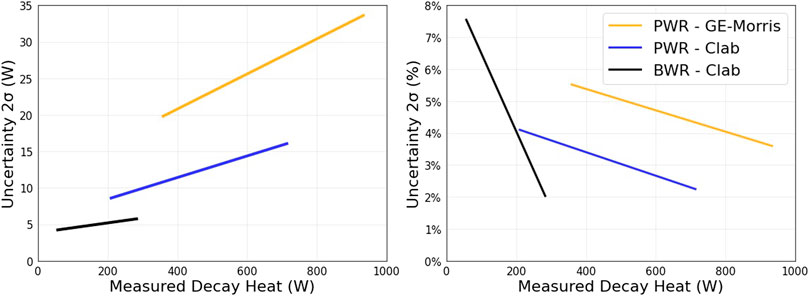
FIGURE 1. Uncertainties in measurements of the analyzed SFAs.

3 Calculational methods

The decay heat calculations are performed using the SCALE nuclear modeling and simulation code system (Bearden and Jessee, 2018) (version 6.2.3). The SCALE package is widely used in nuclear system design, safety analyses, and LWR analyses. The SCALE multi-group library (56-group structure) has reduced computational requirements and is suitable for the current application. The decay and fission yield data are based on the ENDF/B-VII.1 nuclear data library (Chadwick et al., 2011), while the libraries of the multi-group (MG) cross-section data (XS) are based primarily on ENDF/B-VII.1 along with supplementary data from the JEFF-3.0/A nuclear data library.

3.1 Decay heat calculations

The current study calculations relied on the SCALE code system’s Polaris and ORIGEN codes for concurrent verification. Both codes differ in their methods, approximations, and the details of spatial modeling. The validation of Polaris and ORIGEN was conducted previously (Shama et al., 2022) and furtherly analyzed in the current study. Polaris is a lattice physics module commonly used for the analysis of LWR FAs (Jessee et al., 2021; Mertyurek et al., 2021). The module performs lattice calculations coupled with ORIGEN for depletion and decay calculations. Polaris calculates the SFA decay heat, along with the nuclide-wise contributions. The ORIGEN calculations follow the steps: 1) generation of lattice-specific irradiation-dependent XS data using TRITON (DeHart and Bowman, 2011; Bearden and Jessee, 2018), 2) followed by XS interpolations using the ARP utility, 3) followed by depletion and decay calculations using ORIGEN. ORIGEN uses the interpolated XS data, the total material of the FA (both the fuel and the cladding and spacers), along with cycle-wise power densities and lengths. The ORIGEN calculations were added because of the large experience accumulated worldwide, and to be in a condition to verify the results and conclusions based on the Polaris calculations.

The models of both Polaris and TRITON are 2D layouts representing the active section of the FAs. The 2D models are axially symmetric, implementing reflective boundary conditions (radially) and excluding the neighboring assemblies. Also, the irradiation history resolution is at the level of cycle-average values, as provided in the reference (SKB, 2006). Downstream TRITON, ORIGEN is used, which is a zero-dimension code.

3.2 Uncertainty analyses

Stochastic propagation of uncertainties in calculations of SNF characteristics is commonly applied in literature (Leray et al., 2016; Rochman et al., 2016; 2018; Ilas and Liljenfeldt, 2017). In the present study, calculated uncertainties and correlations are obtained through stochastic propagation of uncertainties in the nuclear data (ND) and the SFA design and operational parameters (DO). The Sampler super-sequence of the SCALE package was used along with Polaris and ORIGEN calculational sequences. Sampler performs stochastic uncertainty propagations, generating and running hundreds of input files of subsequences (e.g., Polaris) and analyzing the outputs (Williams et al., 2013). The subsequence iteratively uses ND and DO parameters obtained through random sampling. Nuclear data are sampled from the ND covariances (available in SCALE), and the DO parameters are sampled from their joint probability distributions. The outputs are distributions of the calculated decay heat values, allowing uncertainties and correlations to be calculated.

The considered ND uncertainties are fission yield (FY) and XS uncertainties. These uncertainties are available in the SCALE code system, based primarily on the ENDF/B-VII.1 nuclear data. ENDF/B-VII.1 covariance data and other supplementary data are sources for the XS covariances. Fission yield variances (combining independent and cumulative yields) are sources for the FY covariances.

The DO uncertainties are based on literature values (NEA, 2016). The implemented uncertainties are similar to the ones implemented in a previous study (Shama et al., 2021), which excludes uncertainties in parameters such as the gap between assemblies and the rod-to-rod pitch considering their negligible contribution to the calculated uncertainties. The uncertainties of the DO parameters around their means were assumed to follow normal distributions bounded by ±3 $\sigma$. The form of the distribution, normal vs. uniform, has shown little relevance toward calculated decay heat uncertainties compared to the variance of the distribution (Shama et al., 2021).

The heavy-metal mass of the FA is assumed to be precise, and a negative correlation between the cross-sectional area of all fuel rods and the fuel density is implemented. U-235 enrichments of all rods are assumed to be fully correlated. Fuel temperatures, water densities and temperatures, void fractions, and the boron content in the water are the same throughout the lattice. In different cycles, these parameters are assumed to be fully correlated. The cycle average power densities are assumed to be normally distributed with a standard deviation of 1.67%. They are also assumed to be fully correlated between cycles, resulting in a burnup uncertainty of 1.67%. A full inverse correlation was assumed between the water density and temperature for the PWRs. For the BWRs, the water temperature is constant, and the water density variance originates from the void fraction variance. Also, a full correlation was assumed between the power density and fuel temperature in the PWR and BWR FAs.

The DO parameters can vary significantly along the FAs and during the irradiation cycles. However, the implemented DO values and their uncertainties are assembly-wise and cycle-wise averages rather than local or instantaneous ones. For instance, the void fraction in the BWRs changes axially, and the implemented nominal and uncertainty values are axial averages. Similarly, the boron content is implemented as cycle averages, which change during the irradiation cycles.

The uncertainty calculations using Polaris are straightforward, as shown in Figure 2. Two independent branches of calculations are performed for the ND and the DO parameters. Then, the decay heat covariances obtained from each branch are combined. The counterpart of ORIGEN proceeds in two steps (Figure 2). Firstly, Sampler is used along with TRITON, similar to the Polaris case, perturbing the ND and the DO parameters independently. The output of TRITON is a library of XS data for each distinct FA design. Combined with Sampler, the output is a library of perturbed XS data for each distinct FA design. Then, using Python programming language (Python Software Foundation, 2022), numerous ARP and ORIGEN inputs are generated, incorporating the perturbed XS data and the perturbed DO parameters. The XS libraries are firstly used downstream in ARP interpolating into the FA-specific XS data, then ORIGEN performs the depletion and decay calculations using these interpolated data. In the ND branch, the various runs of TRITON, ARP, and ORIGEN use the nominal DO parameters. The three codes apply consistent perturbation factors for the DO parameters in the DO branch. The perturbations are 625 for the Polaris models and 400 perturbations for the ORIGEN ones—1250 and 800 considering both ND and DO perturbations.

FIGURE 2

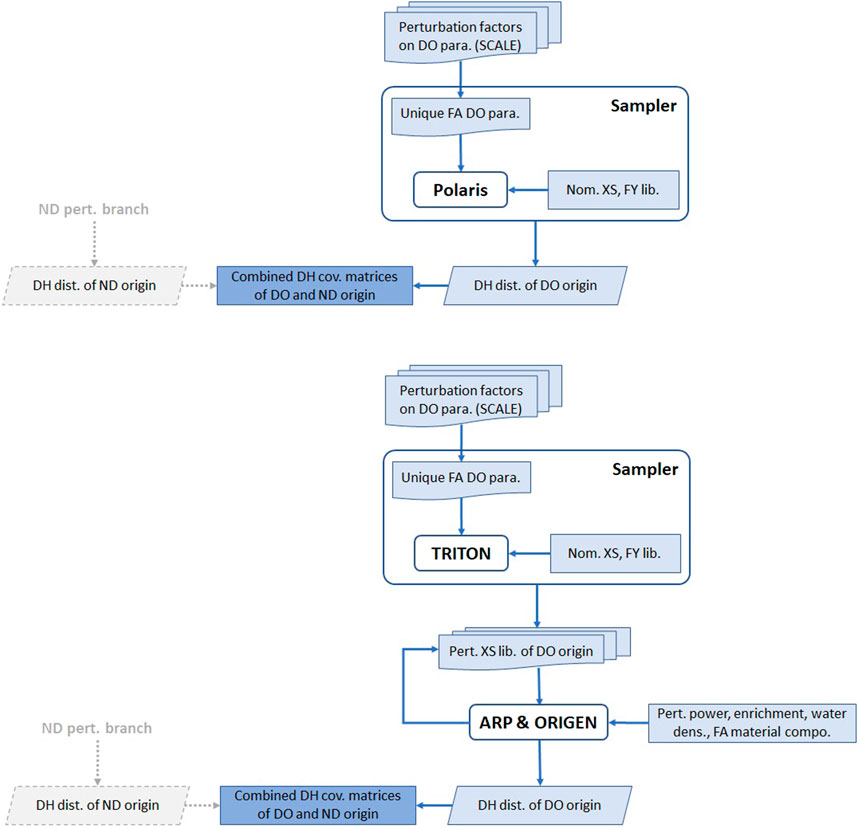
FIGURE 2. Uncertainty calculations using Polaris (top plot) and ORIGEN (bottom plot). The right branch is for the DO parameters, and the left is for the ND.

Not all parameters listed in (Shama et al., 2021) are expressed in the three codes. TRITON implements all these parameters similarly to Polaris. In comparison, ARP and ORIGEN allow only perturbations in a few parameters, such as the power density, enrichment, moderator density, and the balance of the structural materials (in addition to using the TRITON-generated perturbed XS libraries). Similar to the Polaris case, the calculated covariances from the ND and the DO branches are combined.

3.3 Expression of uncertainties

Uncertainties and correlations in both calculations and measurements are considered. Uncertainties in the measurements are shown in Figure 1. The measurements have no reported correlations—an assumed value in the current study. Uncertainties in the calculations are due to independent uncertainties in the ND and the DO parameters, calculated as:

$\sigma =\sqrt{\frac{1}{N-1}{\displaystyle \sum _k^N}{\left({DH}_k-\overline{DH}\right)}^2}(3)$

Where $\overline{DH}$ is the average decay heat and ${DH}_k$ is the decay heat calculated using perturbed ND or DO parameters. Eq. 3 is calculated for both ND and DO parameters. The uncertainties of ND origin are assumed uncorrelated with those of origin from DO parameters. The calculated decay heat uncertainty is obtained as follows:

${\sigma }_C^2\cong {\sigma }_{ND}^2+{\sigma }_{DO}^2(4)$

Also, the errors in the calculations and measurements are assumed uncorrelated. The uncertainty of the bias is calculated as follows:

${\sigma }_B^2\cong {\sigma }_C^2+{\sigma }_E^2(5)$

Correlations of the calculations result from consistently using the same perturbed ND and perturbation factors in all models, calculated as:

$\begin{array}{c}{\rho }_{ij}=\frac{1}{N-1}{\displaystyle \sum _{k=1}^N}\frac{\left({DH}_k^i-{\overline{DH}}_i\right)\left({DH}_k^j-{\overline{DH}}_j\right)}{{\sigma }_i{\sigma }_j}\end{array}(6)$

Where $i$ and $j$ refer to each pair of benchmarks in the validation data.

3.4 Significance of the bias

In the current study, the null hypothesis is that the calculated decay heat and the measured value are equal:

$H_0:C-E=0(7)$

The alternative hypothesis is that they are significantly different: $H_a:C\ne E$. Testing the hypothesis proceeds by calculating a $z$-score (Hayslett and Murphy, 1981; Draper, 2011) for each bias as:

$z_i=\frac{B_i}{{\sigma }_{B,i}}=\frac{C_i-E_i}{{\sigma }_{B,i}}(8)$

The $z$-scores of all the data are weighted and combined using a $z$-transform (Evans, 1996; Stouffer, S. A. et al., 1949):

$\overline{z}=\frac{{\displaystyle {\sum }_{i=1}^N}{w}_i{z}_i}{\sqrt{{\displaystyle \sum _{i=1}^N}{w_i}^2+2{\displaystyle {\sum }_{i<j}^N}{w}_i{w}_j{\rho }_{ij}}}(9)$

Where $w_i$ is the weight for $z_i$, and ${\rho }_{ij}$ is the correlation between $z_i$ and $z_j$. The weights are assumed to be the same in the current study. The correlations were calculated from the covariances as follows:

${\rho }_{ij}=\frac{cov\left(B_i,B_j\right)}{{\sigma }_{B,i}{\sigma }_{B,j}}(10)$

Eq. 10 uses the covariance data of both calculations and measurements. The latter covariances are calculated assuming different levels of correlations between the benchmarks. Low correlations between measurements or calculations in Eq. 10 would result in a higher combined $z$-score, easing the rejection of the null hypothesis, i.e., the test is conservative. The availability of covariance information between measurements could reduce this conservatism.

4 Bias predictions of the random forest

The present study uses ML algorithms based on RF models to predict the bias. The RF models (Breiman, 2001) are built using numerous regression trees obtained by sampling from the data, reducing the variance of the predictions. Within each tree, the target response of an observation is obtained by averaging the response values of the observations in the same terminal node, i.e., RF models are localized regression or weighted neighborhood schemes (Lin and Jeon, 2002). A terminal node is an interval in the predictor space where the target response is approximated to have a constant value. Predicting the response of $x$, located in a terminal node containing $N$ observations, proceeds as following:

$\widehat{y}\left(x\right)=\frac{1}{N}{\displaystyle {\sum }_{n=1}^N}{y}_n.w_{\left(x,\acute{x}\right)}(11)$

Here, the weight $w_{\left(x,\acute{x}\right)}$ is one if the observation is located in the same terminal node as $\acute{x}$, and zero otherwise. The predictions of many trees are combined, e.g., weighted by their out-of-bag estimate.

The design matrix in the current study contains only one variable: the correlation between benchmarks. In this learning setting, the node containing the unit correlation is used for the bias prediction of the target benchmark. The target benchmark and the application case are always located at unit correlation. In applying the RF model, the predicted bias is the average bias of highly similar benchmarks located within a correlation interval from unity $\left[co,1\right]$. Here, $co$ is a cutoff correlation above which benchmarks contribute to the bias prediction of the target benchmark or the application case. The cutoff correlation is also a variable that depends on the data. The predicted bias at the unit correlation $\left(B_{\rho =1}\right)$ using $K$ trees, each having weight $w_k$, is obtained as follows:

$B_{\rho =1}=\frac{1}{N}{\displaystyle {\sum }_{n=1}^N}{w_{k}B}_k.I_{\rho \in \left[co,1\right]}\left(\rho \right)(12)$

Here, the sum of weights is unity.

4.1 ML algorithm

The RF model is applied within the algorithm shown in Figure 3. The data contain 167 measurements conducted on 98 unique SFAs (several SFAs have multiple measurements). The algorithm starts with a random sample of benchmarks, considering only one measurement for each SFA. The algorithm is repeated by considering numerous random samples. Within each iteration, the correlation matrix is divided into 98 correlation vectors. The bias at unit correlation is used as a test sample. An RF model is obtained on the remaining section of the bias and the correlation vector (the design matrix). The RF model is used to predict the bias at unit correlation. The process resembles the leave-one-out cross-validation procedure (LOOCV) (Raschka, 2020), providing an estimate of the test error.

FIGURE 3

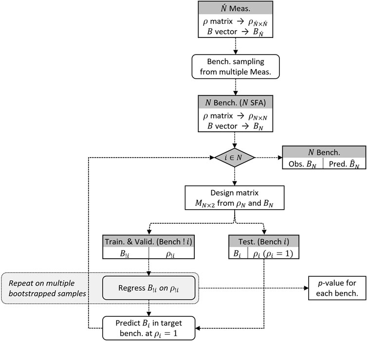
FIGURE 3. The ML algorithm starts with bias and correlation. The algorithm is repeated for random samples of benchmarks, i.e., sampling a single measurement from each SFA.

The main outcome of the algorithm is a vector of bias predictions (corresponding to the original bias of the random sample of benchmarks). Aggregated measures are obtained for assessment of the bias-predictive performance, such as:

1. The coefficient of determination $R^2$ (Wright, 1921).

2. The root-mean-square-error (RMSE) (Willmott, 1981).

3. The p-value of the two-sample Kolmogorov–Smirnov test (KS test) (Daniel, 1990).

A secondary outcome of the algorithm is the p-value of each benchmark obtained from the regressed model on the training and validation data. The aggregated p-values are used in outliers analyses.

5 Results

The bias prediction results are presented in this section. Firstly, the data generated for the ML application are provided. The validation bias, the parameter required to be predicted, is provided in Section 5.1. The correlation matrix, the parameter used to learn the validation bias, is provided in Section 5.3. Sections 5.2, 5.4 were also included to give the uncertainty analyses results used to generate the correlation data and statistical analysis of the significance of the validation bias using the collected uncertainty and correlation data. The last sections address the ML bias-predictive performance, potential outliers, interpretation of the ML models, differentiation between validation data having different uncertainties, and verification of the ML results using the Bayesian approach.

5.1 Validation results

The validation results in this study are updates of the ones provided in (Shama et al., 2022), listed in Table 1. The average Polaris bias of the PWRs is the same as the one in (Shama et al., 2022). For the BWRs, it is 0.1 W less, accounting for the inclusion of FA 2118 to the data (Barsebäck-1 reactor) and more detailed geometry representations of 4 FAs from the Ringhals-1 and Barsebäck-1 and 2 reactors. For ORIGEN, the current results are significantly different from the ones in (Shama et al., 2022) for the FAs of Ringhals-1, Barsebäck-1, Oskarshamn-2, San Onofre-1, and Point Beach-2, considering more accurate irradiation histories and lattice geometry representations in TRITON. The calculations using TRITON are computationally intensive and necessitated simplifications such as excluding corner and edge rods having reduced diameters. In the current study, a more detailed representation of the models is followed in the TRITON calculations.

TABLE 1

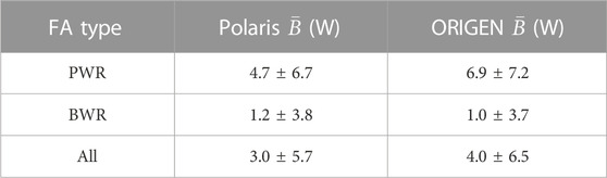
TABLE 1. Average biases of Polaris and ORIGEN, along with one standard deviation (1 $\sigma$) considering the variance of the data.

Polaris and ORIGEN provide calculated decay heat values approximately 5 and 7 W higher than the measurements of the PWRs, respectively. The corresponding bias for both codes is ∼1 W for the BWRs. Such performance could be satisfactory for several applications. However, fluctuations are significantly large, resulting in 1 $\sigma$ of approximately 6 W, evaluated on all the benchmarks for both Polaris and ORIGEN cases. On average, for the whole data, the calculations are within 1.0%–1.2% of the measurements, along with 1 $\sigma$ of 2.2%.

5.2 Uncertainty analyses

Uncertainties of ND and DO origins were separately propagated in the calculational models for all benchmarks. Then, the covariance matrices resulting from the ND and DO uncertainty propagations are summed to obtain a covariance matrix due to the total calculational uncertainties. The uncertainties of ND and DO origins are assumed independent. Differences in the calculated uncertainties and correlations between models perturbing the DO and ND together and the current approach are calculated for the FA F32 of the Ringhals-2 reactor (a PWR FA having 50 GWd/tU burnup) and the FA 1177 of the Ringhals-1 reactor (a BWR FA having 36 GWd/tU burnup). The comparison shows <0.3% and <0.1% differences in the calculated decay heat uncertainties and correlations, respectively, which are considered acceptable approximations in the current study.

The calculated uncertainties are summarized in Table 2, represented as 1 $\sigma$ of the calculated decay heat values. The table lists uncertainties of ND and DO origins along with the total calculated uncertainties. The DO uncertainties result is ∼2% uncertainty in the calculated decay heat for Polaris and ORIGEN, whereas it is <1% due to ND uncertainties. No significant differences are noted between the calculated Polaris and ORIGEN uncertainties and the PWRs and the BWRs. Additionally, both calculated uncertainties show low variances around their averages. These observations indicate that uncertainties of the same origins are propagated in the less-detailed ORIGEN models equivalently to the more-detailed Polaris ones. The TRITON-generated perturbed XS data, and the few model parameters expressed in the ORIGEN model (such as power, burnup, enrichment, and moderator density) are sufficient to express uncertainties equivalently to the more-detailed Polaris models.

TABLE 2

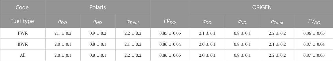
TABLE 2. Averages along with one standard deviation of the calculated uncertainties 1 $\sigma$ (%), both of ND and DO origins, the total calculated uncertainties, and the fractional variances of DO uncertainties.

Uncertainties of different origins could be presented regarding the fractional variance (FV). The contributions of DO uncertainties to the total calculated uncertainties are evaluated as:

$\begin{array}{c}{FV}_{DO}=\frac{{\sigma }_{DO}^2}{{\sigma }_C^2}=\frac{{\sigma }_{DO}^2}{{\sigma }_{ND}^2{+\sigma }_{DO}^2}\end{array}(13)$

The contributions of uncertainties of DO origins to the calculated decay heat uncertainties are listed in Table 3. Similar to the total uncertainties, the differences between the PWRs and the BWRs are insignificant. The uncertainties of DO origins contribute largely to the calculated uncertainties, resulting in ≥85% of the total variance of the calculated decay heat.

TABLE 3

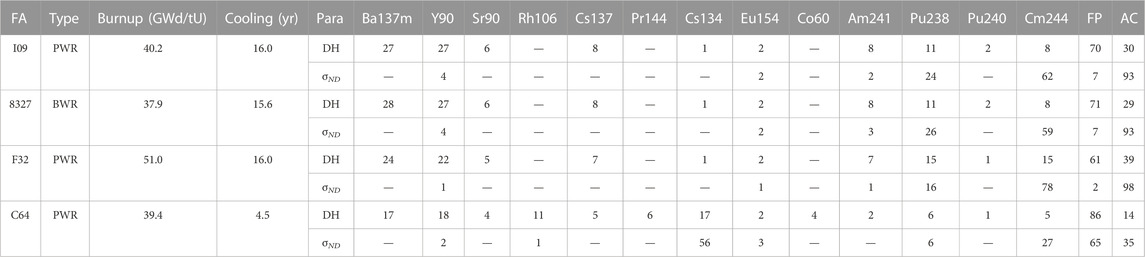
TABLE 3. Selected FAs for analyses of nuclides-wise contributions to the decay heat and the decay heat uncertainty. Contributions from decay heat-relevant nuclides are shown in percentages.

Uncertainties in the FA burnup significantly contribute to the calculated decay heat uncertainties (Shama et al., 2021). The calculated decay heat uncertainties (both of ND and DO origins) and the FVs of DO origins are plotted against the burnup in Figure 4. They both show trends with burnup. On average, the higher the FA burnup, the higher the calculated decay heat uncertainty (for both Polaris and ORIGEN). Also, the FV of DO origins decreases at higher burnups, i.e., uncertainties of ND origin increasingly contribute to decay heat uncertainties at higher burnups.

FIGURE 4

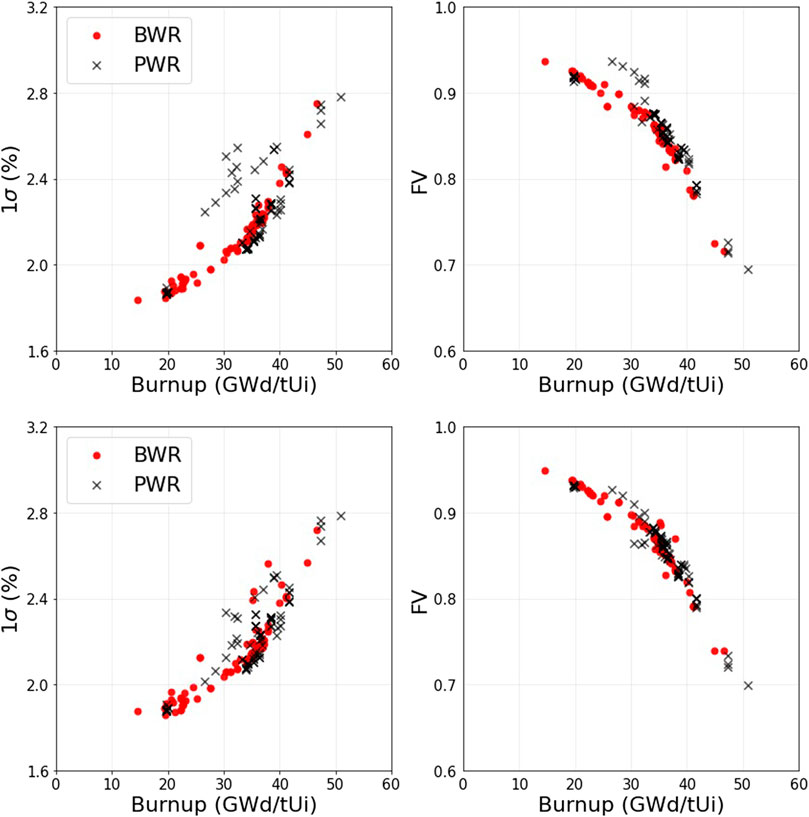
FIGURE 4. Polaris (top) and ORIGEN (bottom) calculated uncertainties of the decay heat (left plots), and the corresponding fractions of variance of DO origins (right plots).

The relevancy of individual uncertainties of the DO parameters toward the calculated decay heat uncertainties is analyzed by examining their correlations. For each benchmark, correlations are calculated between the calculated decay heat (considering both ND and DO uncertainties), and each of the perturbed DO parameters. Figure 5 shows plots of the calculated correlations, indicating that burnup is a highly relevant parameter, significantly and positively correlated with the decay heat for Polaris and ORIGEN. The decay heat tends to show considerably lower correlations with the other DO parameters, except for parameters inducing neutron spectral changes such as the water density and the cladding outer radius. Lower water density or larger cladding outer diameter, lower moderation, and harder spectrum tend to increase the calculated decay heat value in the analyzed benchmarks.

FIGURE 5

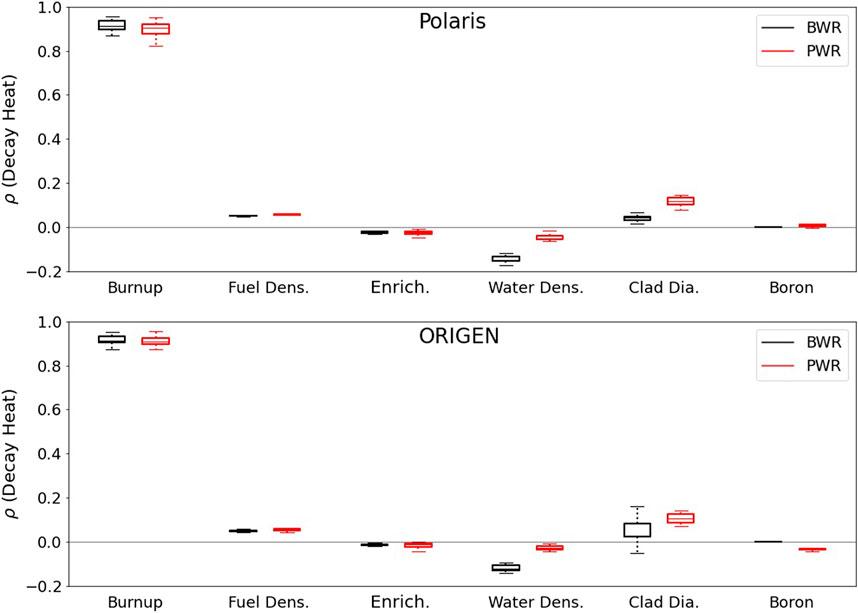
FIGURE 5. Correlations of the calculated decay heat with the perturbed DO parameters. The median, first and third quartiles, and whiskers are shown—whiskers are 1.5 $\times$ interquartile range.

5.3 Correlation matrices

The correlations between the calculated decay heats are obtained for all benchmarks based on perturbations in the ND and the DO parameters. When combined, they form the design matrices used in the ML application. Figure 6 shows the calculated correlations between the decay heats using both Polaris and ORIGEN. The correlation heatmaps are ordered according to the burnup (top to bottom and left to right), e.g., the upper left corners of the maps show the obtained decay heat correlations for assemblies having high burnup values. The lower left corners of the maps show the obtained correlations for assemblies having high burnup values to those having low burnup values. The correlations between the decay heat values are positive and significantly high due to perturbations in both the DO parameters and the combined ND and DO parameters. For Polaris, only 2.5% of the correlations are below 0.51 considering the ND perturbations and 0.87 considering the combined ND and DO perturbations. The corresponding values for ORIGEN are 0.49 and 0.91. Relatively higher correlations are observed between benchmarks having high similarity in their burnup. These high correlations are obtained solely by perturbing the ND, also combined with the DO parameters perturbations. Significant low correlations are observed between several FAs and the rest of the data (low correlation bands across the correlation matrices). Such benchmarks belong to the San Onofre-1 and Point Beach-2 reactors. However, these FAs show notably high correlations among themselves.

FIGURE 6

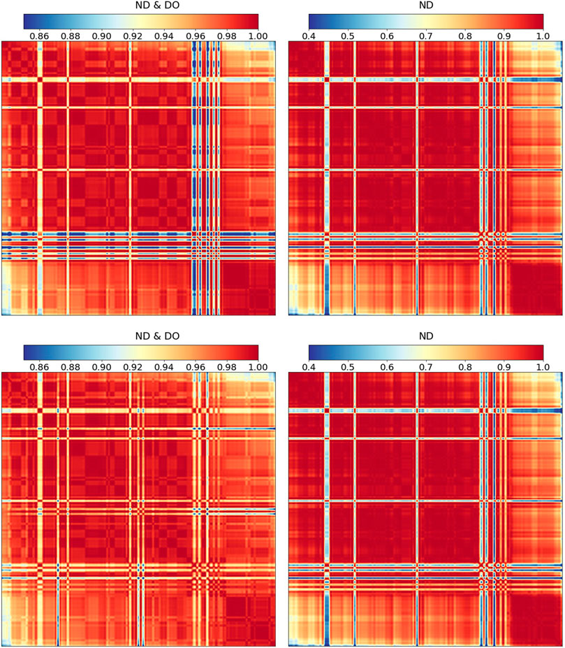
FIGURE 6. Correlations between the calculated decay heats using Polaris (top row), and ORIGEN (bottom row). The left matrices result from perturbing the ND and the DO parameters, whereas the right ones result from perturbing the ND solely. The matrices are ordered according to the burnup (top to bottom and left to right).

The decay heat is an integral value resulting from the nuclear decay of many radionuclides. Differences between the analyzed FAs, such as their burnup and cooling time, change the correlations as they impact nuclide-wise contributions to the decay heat and the decay heat uncertainty differently. Four FAs differing in their characteristics are analyzed (Table 3). The reference FA is I09 (Ringhals-2). The remaining three FAs have the following differences from FA I09:

1. FA 8327 differs in the reactor of origin,

2. FA F32 essentially differs in the burnup,

3. FA C64 essentially differs in the cooling time.

Decay heat-relevant nuclides are analyzed, which produce >99.9% of the decay heat in the analyzed FAs. Table 3 provides their contribution to the decay heat and its uncertainty due to ND perturbations. The contributions from the fission products (FP) and the actinides (AC) are also provided. The FA I09 is the reference case, showing 7% decay heat uncertainty from the FP (mainly Y-90) and 93% from the AC (Pu238, Am241, and Cm244). Relative to FA I09, the remaining three FAs show the following:

1. FA 8327 shows approximately similar contributions from the FP and AC and the nuclide-wise contributions to the decay heat and its uncertainty. Its burnup and cooling time are similar to the reference case.

2. FA F32 shows significantly low contributions from uncertainties in the FP compared to the reference case. Contributions from the Cm-244 nuclide to the decay heat and its uncertainty are considerably higher relative to the reference case. The FA has higher burnup than the reference case, and Cm-244 builds up with burnup in an increasing trend.

3. FA C64 shows significantly high contributions to the decay heat and its uncertainty from the FP. Shorter-lived FP, such as Rh-106 and Cs-134, significantly contribute to the decay heat at short cooling times. Cs-134 alone contributes >50% to the decay heat uncertainty, having a half-life of approximately 2 years. The longer-lived ACs do not contribute as much as the reference case (with respect also to the FP).

5.4 Significance of the validation bias

Comparing the bias to uncertainty allows for testing its significance. Eqs 8, 9 are used to obtain a combined $z$-score for all benchmarks, considering the calculations and measurements’ uncertainties and correlations. Uncertainties and correlations between the calculated decay heat values are presented in Sections 5.2, 5.3. Experimental uncertainties are based on literature (Section 2), whereas the correlations are not available, assumed herein. Independent measurements from two facilities are considered (Clab and GE-Morris); both used the same calorimeter type. The measurements of the Clab facility are assumed to correlate with each other with the same correlation ${\rho }_E$, independent from the measurements at the GE-Morris facility. Similarly, the measurements at the GE-Morris facility are assumed to correlate with each other with the same correlation ${\rho }_E$.

Figure 7 shows the combined $z$-scores of both Polaris and ORIGEN, individually for the PWRs and the BWRs. The plot shows the variation of the combined $z$-scores over the analyzed range of experimental correlations. Higher correlations between the measurements reduce the significance of the calculated combined $z$-scores. Calculating a combined $z$-score using Eq. 9 requires accounting for the correlations between the biases—a summation of the off-diagonal elements of the combined correlation matrix. The summation is positive, considering both the calculated and the measurements’ correlations. This results in a larger denominator in Eq. 9 over the entire range of the measurements’ correlations. The combined $z$-scores could be interpreted to be insignificant over the analyzed measurements’ correlations, considering a two-sided $z$-test with a significance level of 0.05.

FIGURE 7

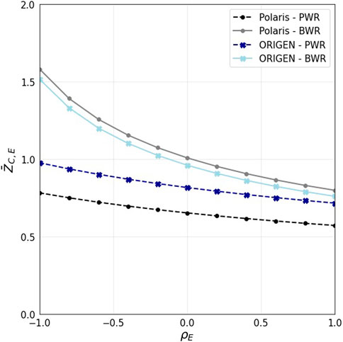
FIGURE 7. Combined z-scores ($\overline{z}$) vs. assumed correlations between the measurements.

5.5 ML predictive performance of the decay heat bias

The decay heat biases are predicted for the Polaris and ORIGEN validation data using the calculated correlations, following the algorithm described in Section 4. The algorithm is implemented using the R programming language (R Core Team, 2022).

For the Clab validation data solely, the predictions show 0.40 and 0.48 reductions of the original variances for Polaris and ORIGEN, respectively. Both reductions in the variances are promising in the current application, and the test errors of both models are 5.0 and 5.9 W, respectively. The test errors are higher for the models using all the data (Clab and GE-Morris benchmarks). Following the algorithm described in Section 4, numerous training and testing iterations are performed, starting each time with a random sample of benchmarks, considering only one measurement for each SFA. Benchmarks highly correlated to multiple calculations on the same SFA show significant variances in their bias predictions. The multiple measurements on the same SFA are typically associated with different biases, sampled iteratively, and contribute to the variance in the predictions of highly correlated benchmarks.

The bias predictions for Polaris and ORIGEN show acceptable KS-test $p$-values. Considering a threshold $p$-value of 0.05, it is failed to reject the null hypothesis that the observed bias and the predicted one have the same distribution. The RF models are promising in their bias predictions, providing biases that bear statistically significant similarity to the observed ones, along with promising reduction of the variance of the validation data.

5.6 Potential outliers

Outliers are referred to as abnormalities or deviants in the data (Aggarwal, 2017), which differ significantly from other observations. They can occur due to systematic or random uncertainties or erroneous data—either erroneous calculations or measurements in the present validation data. Measures of influence (such as Cook’s distance) and hypothesis testing (such as the $z$-test) can detect potential outliers. The $z$-test is used in the current study. The outliers detection in the present study follows the algorithm in Section 4, based on the regressed model onto the training and validation section of the data.

Data points are potential outliers with respect to the data and the model. For such reason, the outliers detection in the current study is selectively conservative, excluding the least number of measurements. Benchmarks are identified as outliers when their aggregate $z$-value is > 3 (corresponding to a threshold significance level of 0.0027). The process is a repeated LOOCV procedure, repeated as a whole and for random benchmark samples. The $p$-values of each benchmark are aggregated, assuming that they are uncorrelated, requiring that the median $p$-value be significant at a threshold significance level of 0.00135. Also, selectively, benchmarks are identified as outliers when detected in both Polaris and ORIGEN validation data.

The outliers analyses are presented in Figure 8. For Polaris, three measurements are detected as outliers, whereas they are four for ORIGEN. Polaris and ORIGEN share two measurements as potential outliers (two measurements on FA 5F2 of Ringhals-3).

FIGURE 8

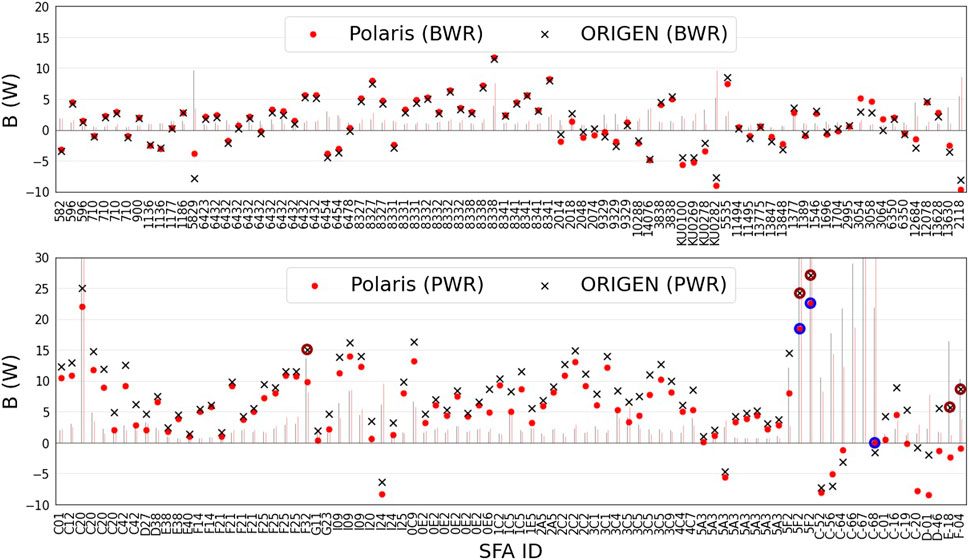
FIGURE 8. The validation biases of Polaris and ORIGEN. The Cook’s distance is shown with bars. The identified outliers are marked with circles (based on their aggregate $z$-score).

The design matrices are reduced, excluding the two detected outliers, and the predictive modeling is redone. The bias prediction results are shown in Figure 9, represented as the predicted bias vs. the observed validation one. The measures in these figures include the reduction, or explanation, of the variances using the RF models applied on the reduced design matrices with respect to the original data without removal of outliers, calculated as:

$R_{final}^2=1-\frac{{\sigma }_{final}^2}{{\sigma }_{initial}^2}(14)$

FIGURE 9

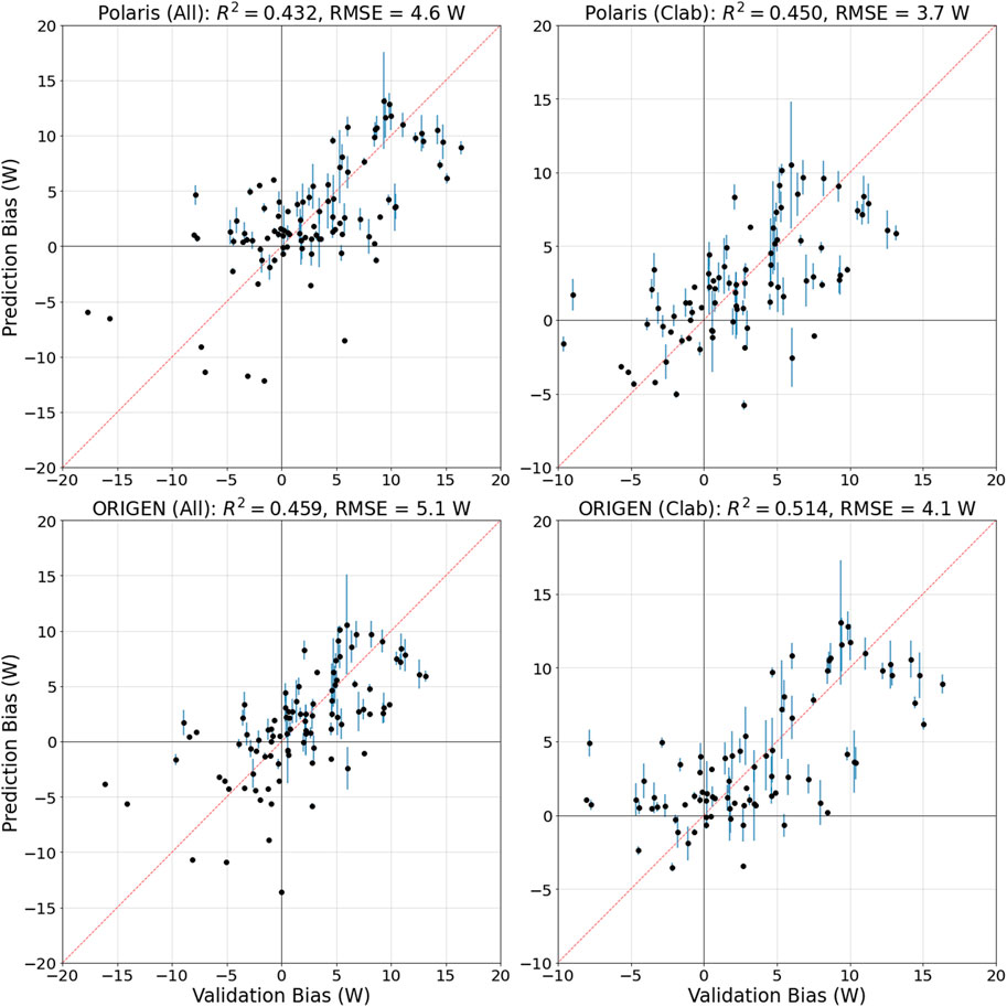
FIGURE 9. The ML predicted bias vs. the observed validation one. The left plots are for the Clab and GE-Morris data, and the right plots are for the Clab data solely. The redline is a 45° line. The validation data exclude two measurements on the 5F2 SFA.

The error bars in Figure 9 are one standard deviation of the predicted biases on the test section of the data. For both Polaris and ORIGEN, excluding the outliers resulted in improvements in the predictive performance of the models. The observation is noted using the Clab data solely, also including the GE-Morris data.

5.7 Interpretation of the models

The validation biases and the predicted ones are shown in Figure 10. The data correspond to the Clab benchmarks solely. Using correlations between benchmarks, the RF model partially explains the observed bias (through the predicted one), reducing the variance. The reductions in the variances are between 0.4 and 0.5, excluding ∼1% of the data as outliers. Initially, Polaris validation shows an overestimation of the measured decay heat by 2.6 ± 4.8 W—considering each FA as an individual benchmark. Then, the RF model results in a bias prediction represented as $f\left(\rho \right)$ ±3.8 W. The followings are concluded:

1. The predicted bias is not necessarily an overestimation. Unlike the validation-based average bias, $f\left(\rho \right)$ is negative for several benchmarks.

2. The fluctuation of the error around the systematic part $f\left(\rho \right)$ is lower than its fluctuation around the average bias for the validation data. The average difference between the validation and the predicted bias is 0.1 W, along with 1 $\sigma$ of 3.8 W.

3. The bias prediction on the target benchmark uses biases of a few highly correlated benchmarks. These informative benchmarks are correlated with the target one above a correlation cutoff. The cutoff itself depends on the data, i.e., it is not constant. The bias is predicted using 2 to 5 benchmarks in 90% and 86% of the Polaris and ORIGEN cases, respectively.

FIGURE 10

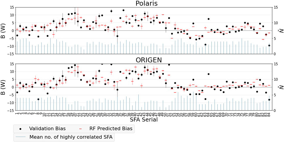
FIGURE 10. Validation and RF predicted biases of Polaris and ORIGEN (only Clab data). The RF predicted bias is based on a few highly correlated benchmarks, denoted by their average number $\overline{N}$.

5.8 Selection of benchmarks for validation

Decay heat-relevant properties differ between the Clab data (lower measurement uncertainties) and GE-Morris data (higher measurement uncertainties). The former data cover burnups between 15 and 51 GWd/tU and cooling times between 11 and 27 years, compared to 27 and 39 GWd/tU and 3 and 8 years for the latter. These differences result in different levels of correlations between the data. Considering the Clab and GE-Morris benchmarks standalone, they correlate significantly within each category, whereas the cross-correlations between the Clab and GE-Morris ones are lower (Figure 11).

FIGURE 11

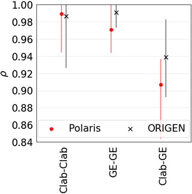
FIGURE 11. Median correlations between the benchmarks of Clab (Clab-Clab), GE-Morris (GE-GE), and between Clab and GE-Morris (Clab-GE). The bars bound 95% of the data.

In the analyzed learning setting, highly correlated benchmarks are used for bias prediction. Including the GE-Morris data would incorporate validation benchmarks having high correlations to discharged FAs with shorter cooling times, i.e., they are closer in the correlation space to applications at shorter cooling times. However, such data are accompanied by higher experimental uncertainties, resulting in higher test errors. Incorporating the GE-Morris data, the RMSE of the predictions increases from 3.7 to 4.6 W. Using neighborhood-based prediction schemes would motivate identifying and addressing sections of the validation data having significant uncertainties.

5.9 Verification against the MOCABA approach

The predictive performance of the ML neighborhood-based scheme is benchmarked against its counterpart of the MOCABA algorithm. MOCABA is a Bayesian update algorithm that utilizes Monte Carlo sampling (Hoefer et al., 2015), which applies to the SNF calculated decay heat as the integral parameter. The prediction of the updated integral parameter using the MOCABA algorithm depends on the similarity between the cases captured using their covariance data. For the application case, the prediction relies more on those cases that share significant covariance with the application. However, in providing predictions, the algorithm is not as localized as the RF model, which implements cutoffs on the correlations between the cases. The algorithm is also applied using the R programming language (R Core Team, 2022).

Figure 12 shows the bias predictions obtained using the MOCABA algorithm, following the overall algorithm described in Section 4. The algorithm is applied, excluding the two outliers identified in Section 5.6. For Polaris and ORIGEN and the two analyzed datasets, the more localized RF model yielded variance reductions in the range of 0.43–0.51, compared to 0.28 to 0.43 for the MOCABA algorithm. The test errors of the RF models (3.7–5.1 W) are also lower than those of the MOCABA algorithm (6.1–9.1 W). Nevertheless, considering the acceptable KS-test $p$-values of both methods, they are both promising bias-predictive methods in the current application. The MOCABA algorithm is more utilized in literature in applications like CSA, and the RF model also weights highly similar cases (even more localized) and shows better predictive performance.

FIGURE 12

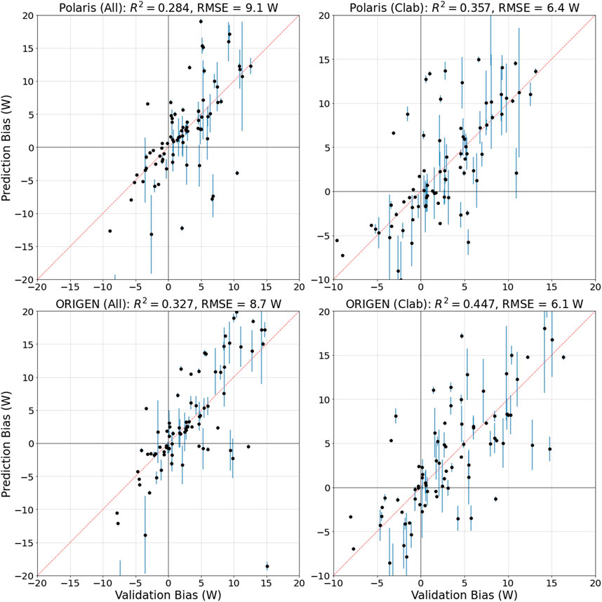
FIGURE 12. Same as Figure 9 using the MOCABA algorithm.

6 Conclusion

The study presents analyses of two hypotheses that the validation bias of SNF decay heat can be shown to be insignificant using uncertainty data and also be predicted using correlation data. The Polaris and ORIGEN codes of the SCALE code system were validated using published measurements performed at the Clab and GE-Morris facilities. Uncertainties and correlations between the decay heats were calculated, perturbing the nuclear data, fuel design, and operational parameters. The validation, uncertainty, correlation, and bias prediction results of both Polaris and ORIGEN show similarities.

The biases have not shown statistical significance, considering uncertainties and correlations. Such a conclusion supports the validation of both codes in SNF decay heat calculations. The study also shows that the considered benchmarks are highly correlated. Fuel assemblies showing similarity in their burnup and cooling time have significantly high correlated decay heats. High correlations resulted in promising bias predictive performance in the application of machine learning algorithms. Such conclusion suggests that the area-of-applicability of the validation data could be constructed using correlations, consequentially burnup and cooling time, which is recommended for future work.

The application of machine learning algorithms, random forest (RF) models weighting highly correlated benchmarks, resulted in bias predictions that show similarities to the validation bias. The variance of the validation bias was reduced by 0.4–0.5, applying the RF model and excluding two measurements. Few benchmarks (2–5) typically contribute to the target benchmark’s bias prediction. Also, the predictive performance was analyzed using data differing in their sample size and measurement uncertainties. It is lower on data having higher measurement uncertainties at the expense of expanding the validation data into shorter cooling times. The performance of the RF model is benchmarked against its counterpart of the MOCABA Bayesian approach, both showing promising bias-predictive performance, particularly for the more localized RF model.

Data availability statement

The raw data supporting the conclusion of this article will be made available by the authors, without undue reservation.

Author contributions

AS collected the data, performed the analyses, and wrote the first draft of the manuscript. All authors contributed to the conception and design of the study, revised the manuscript, read, and approved the submitted version.

Funding

The authors acknowledge the support of KKG, NEA WPNCS subgroup 12, and the European Union’s Horizon 2020 Research and Innovation Programme, grant agreement No 847593 (project EURAD, Work Package 8).

Conflict of interest

The authors declare that the research was conducted in the absence of any commercial or financial relationships that could be construed as a potential conflict of interest.

Publisher’s note

All claims expressed in this article are solely those of the authors and do not necessarily represent those of their affiliated organizations, or those of the publisher, the editors and the reviewers. Any product that may be evaluated in this article, or claim that may be made by its manufacturer, is not guaranteed or endorsed by the publisher.

Supplementary material

The Supplementary Material for this article can be found online at: https://www.frontiersin.org/articles/10.3389/fenrg.2023.1161076/full#supplementary-material

References

Aggarwal, C. C. (2017). Outlier analysis. Manhattan, NY, USA: Springer International Publishing. doi:10.1007/978-3-319-47578-3

CrossRef Full Text | Google Scholar

Ans, (2017). Validation of neutron transport methods for nuclear criticality safety calculations (ANSI/ANS-8.24 No. ANSI/ANS-8.24). La Grange Park, IL, USA: American Nuclear Society. ANSI/ANS-8.24.

Google Scholar

Bearden, B. T., and Jessee, M. A. (2018). SCALE code system (No. ORNL/TM-2005/39, version 6.2.3). Oak Ridge, TN, USA: Oak Ridge National Laboratory. ORNL/TM-2005/39.

Google Scholar

Breiman, L. (2001). Random forest. Mach. Learn. 45, 5–32. doi:10.1023/A:1010933404324

CrossRef Full Text | Google Scholar

Broadhead, B. L., Rearden, B. T., Hopper, C. M., Wagschal, J. J., and Parks, C. V. (2004). Sensitivity- and uncertainty-based criticality safety validation techniques. Nucl. Sci. Eng. Nucl. Sci. Eng. 146, 340–366. doi:10.13182/NSE03-2

CrossRef Full Text | Google Scholar

Chadwick, M. B., Herman, M., Obložinský, P., Dunn, M. E., Danon, Y., Kahler, A. C., et al. (2011). ENDF/B-VII.1 nuclear data for science and Technology: Cross sections, covariances, fission product yields and decay data. Nucl. Data Sheets, Special Issue ENDF/B-VII.1 Libr. 112, 2887–2996. doi:10.1016/j.nds.2011.11.002

CrossRef Full Text | Google Scholar

Daniel, W. W. (1990). Applied nonparametric statistics. Bethersden, UK: PWS-KENT Pub.

Google Scholar

Dean, J. C., and Tayloe, R. W. (2001). ORNL, ORNL-6698, NUREG/CR-6698. Oak Ridge, TN, USA: ORNL Oak Ridge National Laboratory.Guide for validation of nuclear criticality safety calculational methodology (No. NUREG/CR-6698),

Google Scholar

DeHart, M. D., and Bowman, S. M. (2011). Reactor physics methods and analysis capabilities in SCALE. Nucl. Technol. 174, 196–213. doi:10.13182/NT174-196

CrossRef Full Text | Google Scholar

Draper, N. R. (2011). The cambridge dictionary of statistics. Int. Stat. Rev. 79, 273–274. 4 by B. S. Everitt, A. Skrondal. doi:10.1111/j.1751-5823.2011.00149_2.x

CrossRef Full Text | Google Scholar

Epri, (2020). Phenomena identification and ranking table (PIRT) for decay heat - review of current status and recommendations for future needs (No. 3002018440). Washington, DC, USA: EPRI.

Google Scholar

Evans, J. D. (1996). Straightforward statistics for the behavioral sciences. Pacific Grove, CA, USA: Brooks/Cole Pub. Co.

Google Scholar

Gauld, I. C., Illas, G., Murphy, B. D., and Weber, C. F. (2010). Validation of SCALE 5 decay heat predictions for LWR spent nuclear fuel (No. NUREG/CR-6972. Oak Ridge, TN, USA: ORNL Oak Ridge National Laboratory. ORNL/TM-2008/015).

Google Scholar

Gauld, I., and Mertyurek, U. (2018). Margins for uncertainty in the predicted spent fuel isotopic inventories for BWR burnup Credit (No. NUREG/CR-7251). Oak Ridge, TN, USA: U.S. NRC, ORNL Oak Ridge National Laboratory.

Google Scholar

Grechanuk, P., Rising, M. E., and Palmer, T. S. (2018). Using machine learning methods to predict bias in nuclear criticality safety. J. Comput. Theor. Transp. 47, 552–565. doi:10.1080/23324309.2019.1585877

CrossRef Full Text | Google Scholar

Hayslett, H. T., and Murphy, P. (1981). Statistics. Amsterdam, Netherlands: Elsevier. doi:10.1016/C2013-0-01181-4

CrossRef Full Text | Google Scholar

Hoefer, A., Buss, O., Hennebach, M., Schmid, M., and Porsch, D. (2015). Mocaba: A general Monte Carlo–bayes procedure for improved predictions of integral functions of nuclear data. Ann. Nucl. Energy 77, 514–521. doi:10.1016/j.anucene.2014.11.038

CrossRef Full Text | Google Scholar

Ilas, G., and Liljenfeldt, H. (2017). Decay heat uncertainty for BWR used fuel due to modeling and nuclear data uncertainties. Nucl. Eng. Des. 319, 176–184. doi:10.1016/j.nucengdes.2017.05.009

CrossRef Full Text | Google Scholar

Ilas, G., Gauld, I. C., and Liljenfeldt, H. (2014). Validation of ORIGEN for LWR used fuel decay heat analysis with SCALE. Nucl. Eng. Des. 273, 58–67. doi:10.1016/j.nucengdes.2014.02.026

CrossRef Full Text | Google Scholar

Jansson, P., Bengtsson, M., Bäckström, U., Álvarez-Velarde, F., Čalič, D., Caruso, S., et al. (2022). Blind benchmark exercise for spent nuclear fuel decay heat. Nucl. Sci. Eng. 196, 1125–1145. doi:10.1080/00295639.2022.2053489

CrossRef Full Text | Google Scholar

Jessee, M. A., Wieselquist, W. A., Mertyurek, U., Kim, K. S., Evans, T. M., Hamilton, S. P., et al. (2021). Lattice physics calculations using the embedded self-shielding method in Polaris, Part I: Methods and implementation. Ann. Nucl. Energy 150, 107830. doi:10.1016/j.anucene.2020.107830

CrossRef Full Text | Google Scholar

Leray, O., Rochman, D., Grimm, P., Ferroukhi, H., Vasiliev, A., Hursin, M., et al. (2016). Nuclear data uncertainty propagation on spent fuel nuclide compositions. Ann. Nucl. Energy 94, 603–611. doi:10.1016/j.anucene.2016.03.023

CrossRef Full Text | Google Scholar

Lichtenwalter, J. J., Bowman, S. M., DeHart, M. D., and Hopper, C. M. (1997). Criticality benchmark guide for light-water-reactor. Oak Ridge, TN, USA: ORNL Oak Ridge National Laboratory. Fuel in Transportation and Storage Packages (No. NUREG/CR-6361-ORNL/TM-13211). NUREG/CR-6361 - ORNL/TM-13211.

Google Scholar

Lin, Y., and Jeon, Y. (2002). Random forest and adaptive nearest neighbors. J. Am. Stat. Assoc. 101 (474), 578–590. doi:10.1198/016214505000001230

CrossRef Full Text | Google Scholar

Mertyurek, U., Jessee, M. A., and Betzler, B. R. (2021). Lattice physics calculations using the embedded self-shielding method in polaris, Part II: Benchmark assessment. Ann. Nucl. Energy 150, 107829. doi:10.1016/j.anucene.2020.107829

CrossRef Full Text | Google Scholar

Nagra, (2016). The nagra research, development and demonstration (RD&D) plan for the disposal of radioactive waste in Switzerland (No. Technical report 16-02). Switzerland: Nagra. Technical Report 16-02.

Google Scholar

Nea, (2016). Evaluation guide for the evaluated spent nuclear fuel assay database (SFCOMPO). Paris, France: Organisation for Economic Co-Operation and Development.

Google Scholar

Neudecker, D., Grosskopf, M., Herman, M., Haeck, W., Grechanuk, P., Vander Wiel, S., et al. (2020). Enhancing nuclear data validation analysis by using machine learning. Nucl. Data Sheets 167, 36–60. doi:10.1016/j.nds.2020.07.002

CrossRef Full Text | Google Scholar

Oced, N. E. A. (2023). Bias and correlated data, comparison of methods. Paris, France: to be published.

Google Scholar

Posiva, S. K. B. (2017). Safety functions, performance targets and technical design requirements for a KBS-3V repository - conclusions and recommendations from a joint SKB and Posiva working group Posiva, Finland: Posiva SKB Report 01. ISSN 2489-2742.

Google Scholar

Python Software Foundation (2022). Python v3.0.1 documentation. Wilmington, DE, USA: Python Software Foundation. https://docs.python.org/3.0/ (accessed 17 12, 22).

Google Scholar

R Core Team, (2022). R: A language and environment for statistical computing. Vienna, Austria: R Foundation for Statistical Computing.

Google Scholar

Radulescu, G., Gauld, I. C., Ilas, G., and Wagner, J. C. (2014). Approach for validating actinide and fission product compositions for burnup Credit criticality safety analyses. Nucl. Technol. 188, 154–171. doi:10.13182/NT13-154

CrossRef Full Text | Google Scholar

Radulescu, G., Mueller, D. E., and Wagner, J. C. (2009). Sensitivity and uncertainty analysis of commercial reactor criticals for burnup Credit. Nucl. Technol. 167, 268–287. doi:10.13182/NT09-A8963

CrossRef Full Text | Google Scholar

Raschka, S. (2020). Model evaluation, model selection, and algorithm selection in machine learning. arXiv:1811.12808 [cs, stat] https://arxiv.org/abs/1811.12808.

Google Scholar

Rochman, D. A., Vasiliev, A., Dokhane, A., and Ferroukhi, H. (2018). Uncertainties for Swiss LWR spent nuclear fuels due to nuclear data. EPJ Nucl. Sci. Technol. 4, 6. doi:10.1051/epjn/2018005

CrossRef Full Text | Google Scholar

Rochman, D., Kromar, M., Munoz, A., Panizo-Prieto, S., Romojaro, P., Schillebeeckx, P., et al. (2023). On the estimation of nuclide inventory and decay heat: A review from the EURAD European project. Submitt. EPJN - Nucl. Sci. Technol. 9. doi:10.1051/epjn/2022055

CrossRef Full Text | Google Scholar

Rochman, D., Vasiliev, A., Ferroukhi, H., Zhu, T., van der Marck, S. C., and Koning, A. J. (2016). Nuclear data uncertainty for criticality-safety: Monte Carlo vs. linear perturbation. Ann. Nucl. Energy 92, 150–160. doi:10.1016/j.anucene.2016.01.042

CrossRef Full Text | Google Scholar

Schmittroth, F. (1984). ORIGEN2 calculations of PWR spent fuel decay heat compared with calorimeter data (No. HEDL-TME-83-32 (UC-85)). Washington, DC, USA: Hanford Engineering Development Laboratory.

Google Scholar

Shama, A. (2022). Data-driven predictive models: Calculational bias in characterization of spent nuclear fuel. Lausanne, Switzerland: Swiss Federal Institute of Technology Lausanne EPFL. doi:10.5075/epfl-thesis-9309

CrossRef Full Text | Google Scholar

Shama, A., Rochman, D., Caruso, S., and Pautz, A. (2022). Validation of spent nuclear fuel decay heat calculations using Polaris, ORIGEN and CASMO5. Ann. Nucl. Energy 165, 108758. doi:10.1016/j.anucene.2021.108758

CrossRef Full Text | Google Scholar

Shama, A., Rochman, D., Pudollek, S., Caruso, S., and Pautz, A. (2021). Uncertainty analyses of spent nuclear fuel decay heat calculations using SCALE modules. Nucl. Eng. Technol. 53, 2816–2829. doi:10.1016/j.net.2021.03.013

CrossRef Full Text | Google Scholar

Siefman, D. J. (2019). Development and application of data assimilation methods in reactor physics. Lausanne, Switzerland: EPFL. doi:10.5075/epfl-thesis-7525

CrossRef Full Text | Google Scholar

Skb, (2006). Measurements of decay heat in spent nuclear fuel at the Swedish interim storage facility. Coimbatore, Tamil Nadu: SKB. Clab (No. ISSN 1402-3091, SKB Rapport R-05-62).

Google Scholar

Stouffer, S. A., Suchman, E. A., Devinney, L. C., Star, S. A., and Williams, R. M. (1949). “The American soldier: Adjustment during Army life,” in Studies in social psychology in world war II (Princeton, NJ, USA: Princeton University Press).

Google Scholar

Wiles, L. E., Lornbardo, N. J., Heeh, C. M., Jenquin, U. P., MichenerWheeler, C. L., Creer, J. M., et al. (1986). BWR spent fuel storage cask performance. Pre-And post-test decay heat, heat transfer, and shielding analyses (No. PNL-5777 vol. II). Richland, WA, USA: Pacific Northwest National Laboratory.

Google Scholar

Williams, M. L., Ilas, G., Jessee, M. A., Rearden, B. T., Wiarda, D., Zwermann, W., et al. (2013). A statistical sampling method for uncertainty analysis with SCALE and XSUSA. Nucl. Technol. 183, 515–526. doi:10.13182/NT12-112

CrossRef Full Text | Google Scholar

Willmott, C. J. (1981). On the validation of models. Phys. Geogr. 2, 184–194. doi:10.1080/02723646.1981.10642213

CrossRef Full Text | Google Scholar

Wright, S. (1921). Correlation and causation. J. Agric. Res. 20, 557–585.

Google Scholar

Yamamoto, T., and Iwahashi, D. (2016). Validation of decay heat calculation results of ORIGEN2.2 and CASMO5 for light water reactor fuel. J. Nucl. Sci. Technol. 53, 2108–2118. doi:10.1080/00223131.2016.1183528

CrossRef Full Text | Google Scholar