On the role of energy infrastructure in the energy transition. Case study of an energy independent and CO2 neutral energy system for Switzerland

1 Introduction

In order to limit global warming to levels below 1.5 °C, a transition to a fossil-free and renewable-based energy system is mandatory (Pörtner et al., 2022).

Governments have taken up this challenge at different levels by setting targets at the global level. The Paris Agreement signed in 2015 sets specific targets to be reached for countries by the so-called energy transition of the energy system. The definition of transition plans to reach those targets requires decision support tools to identify suitable energy system configurations. Transforming the fossil-based energy system into a new one based on the massive use of renewable energy is challenging, considering the diffuse and intermittent nature of renewable resources. The energy system configuration constitutes interconnected harvesting, conversion, and storage technologies for which installed capacities and strategies of operation need to be defined to satisfy the demands and reach the targets defined as constraints (emission limits) and/or objectives (e.g., economic value). The energy infrastructure is the energy system element that organizes the exchanges (flows) in the system. It is of significant importance as it contributes not only to the energy supply but also to energy management via the interconnection to the storage capacities in the system. The energy infrastructure is also a key element to guarantee the security of supply.

Investments in the energy infrastructure will result in higher energy prices for consumers. In Switzerland, the electrical grid infrastructure accounts for 40% of the electricity price. For other energy services, e.g., mobility in Switzerland, the electrical grid infrastructure accounts for 35% of the final price (Eidgenössische Elektrizitätskommission ElCom, 2021).

With the increase of renewable energy and reduction of fossil imports, the energy infrastructure consisting of grids and storage technologies will be more solicited with the possible need for grid reinforcement. Therefore, it is necessary to model the energy infrastructure as part of the energy systems to represent the infrastructure constraints on the technological choices for energy transition.

For a given system boundary, the energy system model aims to characterize a collection of system states. States are defined by the flows exchanged in the system and the content of different tanks. The collection of states is defined by a list of assumed conditions that will apply to the system and its evolution. Energy system models are mainly mass and energy balance models, where conversion technologies are activated to balance demands with resources. Decisions of the technologies activated in the energy system are either fixed by heuristic rules and experts’ judgment or by using optimization techniques where the experts choose the objective function (e.g., system cost) that drives the energy system evolution. Energy system models are progressively transitioning from simulation (Lapillonne, 1978) to optimization (Fishbone and Abilock, 1981; Schrattenholzer, 1981), a lot of them being open-source. For example, the database of The Open Energy Modelling Initiative (Richstein, 2022) presents a collection of 85 open source models with different times and regional scopes, of which 46 claim to use optimization.

The question of modeling infrastructure and storage was tackled in three principal ways: 1) assessing the role of storage, 2) modeling the grids with losses and regional differences, and 3) comparing multi-energy models.

The transition toward renewable energy-driven energy systems leads to further development to assess surplus energy storage. Antenucci et al. (2019) combined the power system model EMPIRE with the network simulating model NSM to simulate the security of supply challenges in combination with renewable energy storage. Welsch et al. (2015) focused on optimizing intermittent wind energy, combined with the security of supply effect on storage. Another approach combining batteries with PV and the transmission network was achieved by Gupta et al. (2021b). With the emergence of high computing capacities, there is a trend to use such models today to assess uncertainties in optimization strategies; Limpens et al. (2019) modeled the grid as technology-related induced additional cost, Reza Norouzi et al. (2014) elaborated on short-term hydro planning including thermal storage, and Garrison et al. (2018) simulated the security of the supply and dispatch model of renewable electric energy.

While traditional models assume single-point production and consumption, only in recent years have the approaches to quit the copper-plate assumption been made by integrating infrastructure and losses for the power system. Bartlett et al. (2018) focused on the use of hydro power within the electric grid, Abrell et al. (2019) modeled the electric grid for assessing the operation based on the influence of the electric market, Zeljko et al. (2020) estimated the necessary expansion of the electric grid, and Dujardin et al., (2021) estimated the electric grid reinforcement to reach a fully renewable Swiss power system.

Approaches integrating several energy vectors without their infrastructure are either considered singular vectors (Antenucci et al., 2019) or are based on simulation models (Gholizadeh et al., 2019).

Integrating other energy vectors besides electricity was conducted in early modeling years by Fishbone and Abilock (1981) and Manne and Wene (1992) based on the MARKAL model. The application to other energy vectors has been achieved on the fossil fuel infrastructure (Staffell et al., 2019) to determine the role of hydrogen in future energy systems, competing with methane such as Antenucci et al. (2019) linking a mixed-integer linear programming (MILP) power model to the NSM model for assessing the role of security of power supply, or Witek and Uilhoorn (2021) modeling the effect of gas infrastructure failure probability on the risk of supply. Combining different vectors with their corresponding infrastructure has been modeled by Capellán-Pérez et al. (2019), focusing on the post-calculation of the energy return in investment; Li and Zheng (2021) assessed the amplitude of sectors on the security of supply and Capros and E3MLab, ICCS, NTUA. (2013) with the development of the Primes model.

Recent research focuses on securing power infrastructure due to the transition to electrification and intermittency. The target lies in identifying bottlenecks and localizing grid enforcement points to respond to the power production variation of the intermittent resources. The main research focuses on the power system; the identified gap lies in assessing this issue using hydrogen and methane as additional energy vector grids and modeling their distribution and storage infrastructure (Table 1). The most recent example is Hampp et al., (2023, which added different chemical carriers to the existing electric grid model, the PyPSA model (Hörsch et al., 2018).

TABLE 1

TABLE 1. National and international energy system model selection of grid integration overview. Selection based on the number of vectors and grids considered.

energy vector not considered,

energy vector considered, and

energy vector considered and respective grid modeled.

Current research assesses the interplay between individual intermittent resources and their respective storage possibilities, but the global energy system has not been analyzed, where all end uses demands, all energetic resources, and their conversion, storage, and distribution infrastructure have been modeled as constraints at a similar level.

Based on these gaps, the following research questions can be stated:

• How to model different energy grid infrastructures at a common level in global energy systems?

• What is the technical and economic importance of infrastructure reinforcement in energy systems with high shares of renewable energy?

• How does infrastructure reinforcement constrain the deployment of high shares of renewable energy in energy system configurations?

• What is the impact of choices in renewable energy resources and energy conversion and storage (e.g., PV and wind deployment) on the energy infrastructure?

In this study, we complement the EnergyScope models at a monthly basis (Moret et al., 2017; Li et al., 2020; Schnidrig et al., 2021) to represent the infrastructure needed in energy system modeling within the energy transition to show 1) the technical constraints related to the energy system and 2) the necessary investments. This approach will provide answers to the identified gaps by

1. Characterizing and modeling different grid and storage infrastructures in a multi-energy global energy system model and calibrating and validating it using the energy system model of Switzerland in 2020 and its existing grid and storage infrastructure.

2. Investigating the energy infrastructure reinforcement needed from an economic perspective to reach a carbon-neutral and energy-independent Switzerland in 2050.

3. Investigating the grid’s reinforcement constraints and how it influences energy conversion and storage technology choices.

4. Analyzing the interplay between solar photovoltaics/wind and the effect on the grid by parametrizing the deployment of PV.

2 Materials and methods

2.1 Grid separation

Electrical, methane, and hydrogen infrastructures have been modeled, each split into four power levels (e.g., voltage in electric and pressure in gas grids), characterized by the distributed power capacity ${{\mathbf{S}}_{\mathbf{g}}}^{\max }[{\mathrm{G}\mathrm{W}}^{\mathrm{i}\mathrm{n}\mathrm{s}\mathrm{t}}]$, following the discretization of Swissgrid (2020) for the electric and that of Swissgas (2018) for the gas grid.

The conversion technologies connect as producers or consumers to predefined levels in the grid infrastructure. Transformers allow connections between different grids in the same infrastructure. For each grid in the infrastructure, we will calculate the length of the grid and the capacity, defined as the maximum power it can transfer, which will be converted into a diameter of the pipe or cable to be installed. For each grid, a loss model will be used to represent the distribution losses (Figure 1). The infrastructure cost will be calculated as a function of the installed capacity and the length of the distribution grid. In addition, transformation losses and energy recovery will be added for the transformers. Table 2 presents the different grids considered in this study.

FIGURE 1

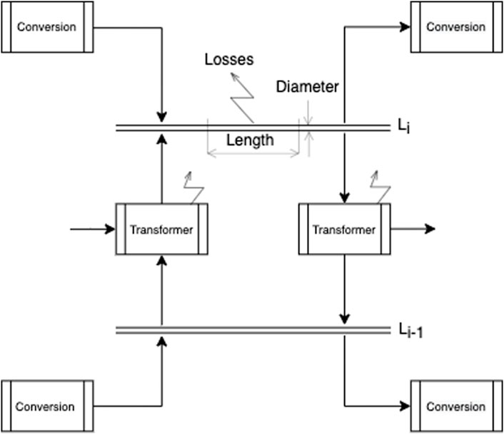
FIGURE 1. Representation of the infrastructure with different levels.

TABLE 2

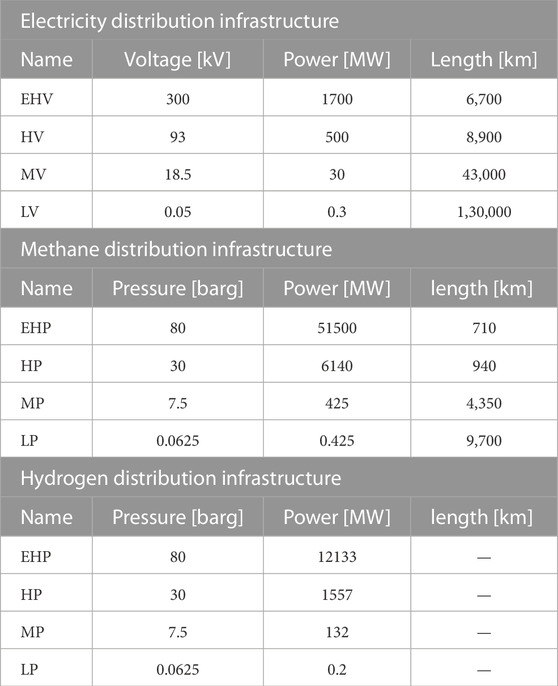
TABLE 2. Grid levels considered for the different infrastructures, power refers to the typical size of the technologies to be connected to the grid level, and length refers to the length considered for the corresponding grid level.

2.2 Grid characterization

2.2.1 Resolution differences

Energy system modeling involves creating digital twins of energy systems to analyze them by integrating various technical and economic assumptions. The link from the real-world dimension to the computer model can be determined by integrating scaling factors ${\mathit{k}}_{\mathit{g}}^{\mathit{i}\leftrightarrow \mathit{j}}$ (Figure 2). The link between the real-world installation and the observed power ${\mathit{k}}_{\mathit{g}}^{\mathit{P}\leftrightarrow \mathit{S}}$ corresponds to the integration of a security coefficient by an engineer, deciding over the transformer size ${\mathbf{S}}_{\mathbf{g}}^{\mathit{inst}}$ by observing the maximum power in the grid $P_g^i$. This power can be modeled in the digital twin of the energy system ${\dot{\mathbf{E}}}_{\mathbf{g}}^{\mathbf{s}}$, which is linked to the maximum power in the grid P_g via the scaling factor ${\mathit{k}}_{\mathit{g}}^{\mathit{P}\leftrightarrow \mathit{S}}$, representing the temporal resolution difference between reality and the model.

${\mathbf{S}}_{\mathbf{g}}^{\mathbf{inst}}={\mathit{k}}_{\mathit{g}}^{\dot{\mathit{E}}\leftrightarrow \mathit{P}}\cdot {\mathit{k}}_{\mathit{g}}^{\mathit{P}\leftrightarrow \mathit{S}}\cdot {\dot{\mathbf{E}}}_{\mathbf{g}}^{\mathbf{s}}.(1)$

FIGURE 2

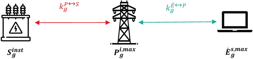
FIGURE 2. Installation size ${\mathbf{S}}_{\mathbf{g}}^{\mathit{inst}}[{\mathrm{G}\mathrm{W}}^{\mathrm{i}\mathrm{n}\mathrm{s}\mathrm{t}}]$, observed power P_g [GW^15min], and modeled power ${\dot{\mathbf{E}}}_{\mathbf{g}}^{\mathbf{s}}[{\mathrm{G}\mathrm{W}}^{\mathrm{T}\mathrm{P}}]$ linking the procedure with scaling factors ${\mathit{k}}_{\mathit{g}}^{\dot{\mathit{E}}\leftrightarrow \mathit{P}}$ and ${\mathit{k}}_{\mathit{g}}^{\mathit{P}\leftrightarrow \mathit{S}}$, represented through electric grid transformer installation.

The scaling factors can be determined using historical data. While the observed power is expressed by a 15 min average power, the temporal resolution ratio between the measured and the modeled power varies for transmission and distribution (Figure 2), which can be summarized to $2_{-0.11}^{+0.76}$ continuous uniform distribution, being considered in the sensitivity analysis.

The security coefficient between observation and installation is estimated by comparing the measured data $P_g^{\mathit{meas}}[{\mathrm{G}\mathrm{W}}^{\mathrm{15}\mathrm{m}\mathrm{i}\mathrm{n}}]$ to the size of the installed transformer. Gupta R. et al., (2021) characterized the Swiss electric grid by discretizing the area of influence of the extra-high-voltage transformers voltage-level-wise to the medium-voltage grid. The identification of the maximum annual power per voltage-level transformer $P_g^{\mathit{meas,max}}$ compared to the transformer installation typical size $S_g^{\mathit{inst}}$ allows estimating the installation security coefficient ${\mathit{k}}_{\mathit{g}}^{\mathit{P}\leftrightarrow \mathit{S}}=3_{-0.40}^{+0.18}$.

2.2.2 Specific length

The specific length corresponds to the average grid length between two conversion stations at the same power level. It depends on the distribution density in a given region and distributed power. For each type of grid, the reference value of distributed power has been considered, and the reference distribution length $({\mathit{l}}_{\mathit{g}}^{\mathit{ref}})$ has been deduced as a function of the consumption density:

${\mathit{l}}_{\mathit{g}}^{\mathit{ref}}=\frac{{\mathit{l}}_{\mathit{g}}^{\mathit{tot}}}{{\mathit{n}}_{\mathit{g}}},\forall g\in \mathcal{G}\mathcal{R}\mathcal{I}\mathcal{D}\mathcal{S},(2)$

where ${\mathit{l}}_{\mathit{g}}^{\mathit{ref}}$ is the mean grid transportation length of grid g [m].${\mathit{l}}_{\mathit{g}}^{\mathit{tot}}$ is the grid length of grid g [m].n_g is the number of consumers in grid g [-].

2.2.2.1 Electric grid

The total length and the number of conversion stations of the grid at the four voltage levels is estimated based on Gupta R. et al. (2021), estimating the electric grid with a top–down approach, down to the MV transformers, allowing calculation of the specific length ${\mathit{l}}_{\mathit{g}}^{\mathit{ref}}$ by adapting Eq. 2

${\mathit{l}}_{\mathit{g}}^{\mathit{ref}}=\frac{{\sum }_i{l}_{g,i}^{\mathit{tot}}}{{\sum }_i{n}_{g,i}},\forall i\in \mathcal{P}\mathcal{O}\mathcal{L}\mathcal{Y}\mathcal{G}\mathcal{O}\mathcal{N}\mathcal{S},g\in \mathcal{G}\mathcal{R}\mathcal{I}\mathcal{D}\mathcal{S},(3)$

where ${\mathit{l}}_{\mathit{g}}^{\mathit{ref}}$ is the mean grid transportation length of grid g [m].$l_{g,i}^{\mathit{tot}}$ is the grid length within a polygon i of grid g [m].n_g,i is the number of consumers in polygon i of grid g [-].

The length and number of consumers of the low-voltage grid are estimated by applying an equidistant distribution of the consumers defined by the national houses and buildings register (Swiss Geoportal, 2019), within the MV Voronoi polygons (Gupta R. et al., 2021). For each MV/LV transformer, the LV grid length can be estimated based on geometric properties, assuming a square area A_i containing grid lines of length l_i connecting the equally distributed points n_i (Eq. 4).

$l_{g,i}^{\mathit{tot}}=\sqrt{A_{g,i}}\cdot \left(\sqrt{n_{g,i}}+1\right),\forall i\in \mathcal{P}\mathcal{O}\mathcal{L}\mathcal{Y}\mathcal{G}\mathcal{O}\mathcal{N}\mathcal{S},(4)$

where $l_{g,i}^{\mathit{tot}}$ is the grid length within a polygon i of grid g [m].A_g,i is the surface of polygon i of grid g [m²].n_g,i is the number of consumers in polygon i of grid g [-].

This approach has been validated by applying the same methodology on HV/MV transformers and estimating the length of the medium-voltage grid for Switzerland’s 1,257 medium-voltage cells (Figure 3). The average error is 2.01%, while the cumulative error is at 23.1%, resulting in R² = 0.913.

FIGURE 3

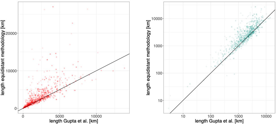
FIGURE 3. Parity plot of the length of the medium-voltage grid, characterized by Gupta R. et al. (2021) and the equidistant method (Eq. 2). Primary errors can be found in polygons of extensive areas compared to the few agglomerations corresponding to alpine and forest environments. The equidistant method distributes the regrouped small agglomerations within the big area, leading to an overestimation of the necessary grid.

2.2.2.2 Gas grids

The calculation of the reference length of the gas grids follows the same procedure as that of the electric grids (Eq. 2). While the number of consumers was known for all electric grid levels and the electric grid length was estimated for three of four levels, the only available information is the extra high pressure (EHP) and high pressure (HP) transmission methane transmission pipeline locations and conversion stations. The distribution network needs to be characterized.

Following the same consumer density approach used for the electric grid, the same splitting of Voronoi polygons has been used. The difference lies in selecting the areas connected to the gas grid. The size of the buffer region around the transmission pipelines was selected as 5 km, such that the number of buildings within the Voronoi polygons adjacent to the buffer region matched the reported 21% of gas grid-connected buildings in Switzerland (Federal Statistical Office, 2017) (Figure 4).

FIGURE 4

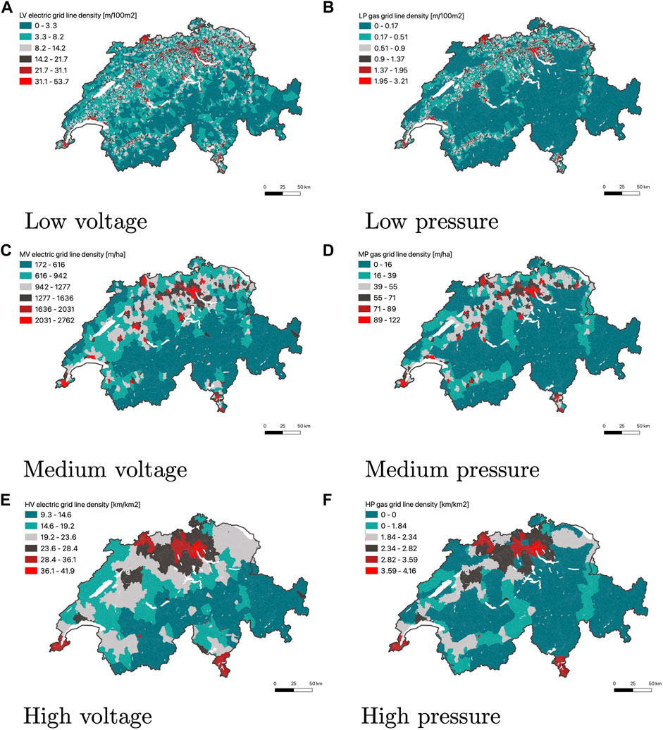
FIGURE 4. Map of Switzerland with the grid line density estimation using the equidistant method (Eqs 2, 4). (A,C,E) show the electric grid polygons. (B,D,F) display the equivalent pressure gas grid Voronoi polygons, within a range of 5 km around the EHP and HP gas grid lines.

This approach is validated by comparing the calculated total lengths to the reported grid lengths, summarized in two levels (Verband der Schweizerischen Gasindustrie VSG, 2020): $>$ 5 bar for transmission (2,243 km) and $<$ 5 bar distribution (17,648 km). Within this case, the transmission pipeline corresponds to the HP and EHP grids, while distribution corresponds to medium pressure (MP) and low pressure (LP) levels. Therefore, summing the equidistant method results leads to a relative error of 26.4% for the transmission grid and 20.3% for the distribution network.

2.2.3 Losses

Each grid g is characterized by the transported distance length ${\mathit{l}}_{\mathit{g}}^{\mathit{ref}}[\mathrm{k}\mathrm{m}]$ and the reference power ${\mathit{S}}_{\mathit{g}}^{\mathit{max}}[{\mathrm{G}\mathrm{W}}^{\mathrm{i}\mathrm{n}\mathrm{s}\mathrm{t}}]$, defining secondary characteristics such as the diameter of the cable or pipe installed and its resistance, defining the linearized specific loss coefficient ${\mathit{\eta }}_{\mathit{g}}^{\mathit{loss}}[\frac{\%}{\mathrm{G}\mathrm{W}\cdot \mathrm{k}\mathrm{m}}]$.

The grid losses depend on the energy flow ${\dot{\mathbf{E}}}_{\mathbf{g}}^{\mathbf{s}}$ within each grid and the respective specific loss coefficient ${\mathit{\eta }}_{\mathit{g}}^{\mathit{loss}}$ (Eq. 5).

The specific loss coefficients in the electric grids $ϵ\in \mathcal{E}\mathcal{L}\mathcal{E}\mathcal{C}-\mathcal{G}\mathcal{R}\mathcal{I}\mathcal{D}\mathcal{S}$ are modeled by the ohmic losses ${\dot{\mathbf{E}}}_{\mathbf{ϵ}}^{\mathbf{loss}}\propto Rϵ\cdot I{ϵ}^2$, with the resistance R being a function of the diameter, length, and specific resistance of the material.

The specific loss coefficients in the gas grid $\pi \in \mathcal{G}\mathcal{A}\mathcal{S}-\mathcal{G}\mathcal{R}\mathcal{I}\mathcal{D}\mathcal{S}$ correspond to a pressure drop within the pipelines. The power loss in gas grids is modeled by the compensation of the pressure drop inside a pipeline, assuming a Poiseuille flow and using the Darcy–Weisbach equation (Howell and Weathers, 1970) ${\dot{\mathbf{E}}}_{\mathbf{\pi }}^{\mathbf{loss}}\propto f_{\pi }^D\cdot {\dot{V}}_{\pi }^2$, where the specific resistance $f_{\pi }^D$ is a function of the pipeline diameter, rugosity, and the density of the transported gas.

${\dot{\mathbf{E}}}_{\mathbf{g}}^{\mathbf{loss}}={\mathit{\eta }}_{\mathit{g}}^{\mathit{loss}}\cdot {\mathit{l}}_{\mathit{g}}^{\mathit{ref}}\cdot {\dot{\mathbf{E}}}_{\mathbf{g}}^{\mathbf{s}},\forall g\in \mathcal{G}\mathcal{R}\mathcal{I}\mathcal{D}\mathcal{S},(5)$

where ${\dot{\mathbf{E}}}_{\mathbf{g}}^{\mathbf{l}\mathbf{o}\mathbf{s}\mathbf{s}}$ is the losses [GW].${\mathit{\eta }}_{\mathit{g}}^{\mathit{loss}}$ is the specific losses $[\frac{\%}{\mathrm{G}\mathrm{W}\cdot \mathrm{k}\mathrm{m}}]$.${\mathit{l}}_{\mathit{g}}^{\mathit{ref}}$ is the grid reference length [m].${\dot{\mathbf{E}}}_{\mathbf{g}}^{\mathbf{s}}$ is the power used [GW].

2.2.4 Costs

Similar to the losses, the investment costs of the grid ${\mathit{c}}_{\mathit{g}}^{\mathit{inv}}[\frac{\mathrm{M}\mathrm{C}\mathrm{H}\mathrm{F}}{\mathrm{k}\mathrm{m}\mathrm{G}\mathrm{W}}]$ mainly depend on the volume to be constructed, and the length is expressed as the installed grid length ${\mathit{l}}_{\mathit{g}}^{\mathit{inst.}}$, while the power capacity S_g [GW] defines the cross-area of the cable (Eq. 6).

${\mathbf{C}}_{\mathbf{g}}^{\mathbf{i}\mathbf{n}\mathbf{v}}={\mathbf{S}}_{\mathbf{g}}^{\mathbf{i}\mathbf{n}\mathbf{s}\mathbf{t}}\cdot {\mathit{c}}_{\mathit{g}}^{\mathit{inv}}\cdot {\mathit{l}}_{\mathit{g}}^{\mathit{inst}}\forall g\in \mathcal{G}\mathcal{R}\mathcal{I}\mathcal{D}\mathcal{S},(6)$

where ${{\mathbf{C}}_{\mathbf{g}}}^{\mathbf{i}\mathbf{n}\mathbf{v}}$ is the investment costs [MCHF].${\mathit{c}}_{\mathit{g}}^{\mathit{inv}}$ is the specific investment costs .$[\frac{\mathrm{M}\mathrm{C}\mathrm{H}\mathrm{F}}{\mathrm{k}\mathrm{m}\mathrm{G}\mathrm{W}}]$${{\mathbf{S}}_{\mathbf{g}}}^{\mathbf{i}\mathbf{n}\mathbf{s}\mathbf{t}}$ is the installation size [GW^inst].${\mathit{l}}_{\mathit{g}}^{\mathit{inst}}$ is the installed grid length [km].

The specific investment cost has been determined using existing projects within Switzerland, validating the assumptions by industrial experts. The detailed calculation can be found in the additional material available in the GitLab repositories.

2.2.5 Grid comparisons

The technology characterization parameters are summarized in Figure 5. The grids are each split into four power levels on a logarithmic scale scatter plot. One can observe that all grids follow the same order of magnitude for power levels and reference lengths and patterns.

FIGURE 5

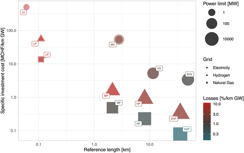
FIGURE 5. Grid infrastructure techno-economic characterization of the electricity (circles), hydrogen (triangles), and methane (squares) grids split into the four power levels: extra high (EH), high (H), medium (M), and low (L) pressure and voltage. Case study for the average Swiss infrastructure. The inner radius corresponds to the minimum power limit, and the outer radius corresponds to the maximum power limit. The specific losses $[\frac{\text{‰}}{\mathrm{G}\mathrm{W}\mathrm{k}\mathrm{m}}]$ are displayed on the logarithmic color scale. The detailed calculation and origin of values can be found on https://gitlab.com/ipese/on-the-role-of-energy-infrastructure-in-the-energy-transition.

The major distinction is visible in the installed power limit S^inst. Gas grids have a higher energy transportation capacity, defined as energy density per grid-length unit, than electric grids. While an EHV grid can transport up to 1.7 GW, EHP hydrogen gas grids can transport 7.1 times more and methane grids 30 times more.

The power limit directly affects the specific cost. While electric grids are more expensive than gas grids, gas grids distinguish due to the respective volumetric energy density, leading to a higher energy density per grid unit length in the methane grid than in the hydrogen grid. The lower energy density leads to higher energy-specific investment costs for the hydrogen grid.

The reference length is in the same order of magnitude for all grids at the same power level. The gas grid’s reference length is constant at each power level as the hydrogen grid is estimated based on the existing methane grid. Despite applying the same methodology to estimate the reference length for the electric and gas grid, the difference as different polygons is considered. While all buildings and polygons were considered connected for the electric grids (Figures 4A, C, E), only the polygons close to the gas transmission pipelines were considered (Figures 4B, D, F). The gas transmission pipelines connect only more densely populated areas, neglecting more rural areas, which leads to lower reference lengths in the gas distribution network.

Regarding operation, the methane grid is also less expensive due to lower losses compensated for by higher compression demands compared to the hydrogen grid. The electric grid losses lie between the two gas distribution grids.

2.3 Linear programming model formulation

The previously described methodology is integrated into EnergyScope (Moret et al., 2017; Li et al., 2020; Schnidrig et al., 2021), a fast-solving energy system model expressed as a mixed-integer linear problem based on energy and mass balance. The decision variables of technology installation size F [GW] and use ${\mathbf{F}}_{\mathbf{t}}[\frac{\mathrm{G}\mathrm{W}{\mathrm{t}}_{\mathrm{T}\mathrm{P}}}{{\mathrm{t}}_{\mathrm{T}\mathrm{P}}}]$ ¹ of each typical period are optimized under different objective functions, subject to environmental, economic, and technical constraints.

2.3.1 Infrastructure design and operation

The necessary infrastructure type $(g\in \mathcal{G}\mathcal{R}\mathcal{I}\mathcal{D}\mathcal{S})$, size F, and operation F_t are defined by the production of the grid-corresponding energy layers $(l(g)\in \mathcal{E}-\mathcal{L}\mathcal{A}\mathcal{Y}\mathcal{E}\mathcal{R}\mathcal{S})$ by the technologies $(tec\in \mathcal{TECHNOLOGIES})$. The operation of the grid during the period t is determined by the sum of the grid-layer-specific outputs of all technologies, which is calculated by multiplying the use of the technology with the corresponding output factor η_out of the desired energy vector layer for each period t (Eq. 7).

$\begin{array}{ll}\hfill {\mathbf{F}}_{\mathbf{t}}\left(g,t\right)\ge & \sum _{\mathit{tec}}{\mathbf{F}}_{\mathbf{t}}\left(tec,t\right)\cdot {\mathit{\eta }}_{\mathit{out}}\left(tec,l\left(g\right)\right)\cdot \frac{1}{\mathit{n}\left(g\right)}\hfill \\ \hfill & \forall g\in \mathcal{G}\mathcal{R}\mathcal{I}\mathcal{D}\mathcal{S}\left(l\right),t\in \mathcal{P}\mathcal{E}\mathcal{R}\mathcal{I}\mathcal{O}\mathcal{D}\mathcal{S},tec\in \mathcal{T}\mathcal{E}\mathcal{C},\hfill \\ \hfill & l\in \mathcal{E}-\mathcal{L}\mathcal{A}\mathcal{Y}\mathcal{E}\mathcal{R}\mathcal{S}.\hfill \end{array}(7)$

The grid installation size is determined by the maximum of the grid operation size over all periods t (Eq. 8).

$\begin{array}{ll}\hfill \mathbf{F}\left(g\right)\ge & {\mathbf{F}}_{\mathbf{t}}\left(g,t\right)\hfill \\ \hfill & \forall g\in \mathcal{G}\mathcal{R}\mathcal{I}\mathcal{D}\mathcal{S},t\in \mathcal{P}\mathcal{E}\mathcal{R}\mathcal{I}\mathcal{O}\mathcal{D}\mathcal{S}.\hfill \end{array}(8)$

The power loss of the grid can be modeled by the multiplication of the operation of the grid, the reference length l_ref(g), and the specific loss coefficient η_Loss(g) (Eq. 9).

$\begin{array}{ll}\hfill {\mathbf{F}}_{\mathbf{t}}^{\mathbf{Loss}}\left(g,t\right)=& {\mathbf{F}}_{\mathbf{t}}\left(g,t\right)\cdot {\mathit{\eta }}_{\mathit{Loss}}\left(g\right)\cdot {\mathit{l}}_{\mathit{ref}}\left(g\right)\hfill \\ \hfill & \forall g\in \mathcal{G}\mathcal{R}\mathcal{I}\mathcal{D}\mathcal{S},t\in \mathcal{P}\mathcal{E}\mathcal{R}\mathcal{I}\mathcal{O}\mathcal{D}\mathcal{S}.\hfill \end{array}(9)$

2.3.2 Energy balance and demand satisfaction

The global annual energy system demands are split into four sectors: households, services, industry, and mobility. Each sector’s energy demand is categorized into electricity (split into four voltage levels): space heating, hot water, process heat, person transport, and freight transport. The transformation of the annual demand in the END USES is summarized in Figure 6. The satisfaction of these demands is achieved through energy conversion technologies, transforming energy and mass layers into other layers with a specific efficiency. The categorization of the technologies is summarized in Figure 7.

FIGURE 6

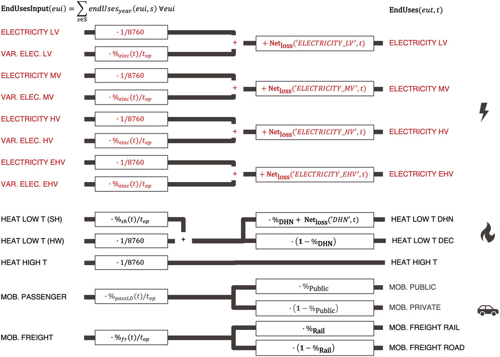
FIGURE 6. Separation and allocation of annual demand into sectoral demands (electricity, heat, and mobility) over time. The red areas represent the changes in the model compared to the original EnergyScope model Moret et al. (2017).

FIGURE 7

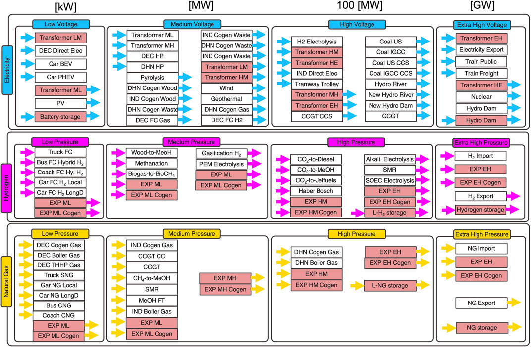
FIGURE 7. Categorization of energy conversion technologies for electricity, methane, and hydrogen networks. The technologies in the red boxes represent the additional infrastructure in the model compared to the original EnergyScope model Moret et al. (2017).

The layer generation balances the end uses by the utilization of technologies and resources F_t, the storage contribution Sto_out − Sto_in, and the compensation of the losses in the grids ${\mathbf{F}}_{\mathbf{t}}^{\mathit{Loss}}$ (Eq. 10). It should be noted that no end uses are defined for the gas layers, leading to a balance between generation, transformation, losses, and storage.

$\begin{array}{ll}\hfill \mathbf{E}\mathbf{N}\mathbf{D}\mathbf{U}\mathbf{S}\mathbf{E}\mathbf{S}\left(l,t\right)=& \sum _{i\in \mathcal{RES}\cup \mathcal{TEC}}{\mathbf{F}}_{\mathbf{t}}\left(i,t\right)\cdot \mathit{\eta }\left(i,l\right)-{\mathbf{F}}_{\mathbf{t}}^{\mathbf{L}\mathbf{o}\mathbf{s}\mathbf{s}}\left(l,t\right)\hfill \\ \hfill & +\sum _{j\in \mathcal{STO}\mathcal{TEC}}{\mathbf{S}\mathbf{t}\mathbf{o}}_{\mathbf{o}\mathbf{u}\mathbf{t}}\left(j,l,t\right)-{\mathbf{S}\mathbf{t}\mathbf{o}}_{\mathbf{i}\mathbf{n}}\left(j,l,t\right).\hfill \end{array}(10)$

2.3.3 Cost and objective function

Following the total cost function C_tot, comprising investment, maintenance, and operating cost, the grid-specific costs comprise maintenance and investment costs (Eq. 11).

Within the investment cost, only the installation of additional technologies is considered. The specific investment cost is multiplied by the difference between the technology installation size F and the existing technology size f_ext. The possibility of the latter difference is smaller than 0, which leads to the necessity to add a slag variable Γ_inv, ensuring the positivity of C_inv for each technology (Eq. 12). Maintenance cost is applied to the total technology size, as defined by Moret et al. (2017) (Eq. 13).

$\begin{array}{ll}\hfill {\mathbf{C}}_{\mathbf{tot}}=& \sum _{\mathit{tec}}\left({\mathbf{C}}_{\mathbf{inv}}\left(tec\right)\cdot \mathit{\tau }\left(tec\right)+{\mathbf{C}}_{\mathbf{maint}}\left(tec\right)\right)+\sum _{\mathit{res}}{\mathbf{C}}_{\mathbf{o}\mathbf{p}}\left(res\right)\hfill \\ \hfill & +\sum _g\left({\mathbf{C}}_{\mathbf{inv}}\left(g\right)\cdot \mathit{\tau }\left(g\right)\right),\hfill \end{array}(11)$

${\mathbf{C}}_{\mathbf{inv}}\left(tec\right)={\mathit{c}}_{\mathit{inv}}\left(tec\right)\cdot \left(\mathbf{F}\left(tec\right)-{\mathit{f}}_{\mathit{ext}}\left(tec\right)\right)+{\mathbf{\Gamma }}_{\mathbf{inv}}\left(tec\right),(12)$

${\mathbf{C}}_{\mathbf{maint}}\left(tec\right)={\mathit{c}}_{\mathit{maint}}\left(tec\right)\cdot \mathbf{F}\left(tec\right),(13)$

${\mathbf{C}}_{\mathbf{o}\mathbf{p}}\left(res\right)=\sum _t{\mathit{c}}_{\mathit{o}\mathit{p}}\left(res\right)\cdot {\mathbf{F}}_{\mathbf{t}}\left(res,t\right)\cdot {\mathit{t}}_{\mathit{o}\mathit{p}}\left(t\right),(14)$

$\forall res\in \mathcal{R}\mathcal{E}\mathcal{S},tec\in \mathcal{T}\mathcal{E}\mathcal{C},t\in \mathcal{P}\mathcal{E}\mathcal{R}\mathcal{I}\mathcal{O}\mathcal{D}\mathcal{S},$

The investment cost of the grid is calculated by multiplying the specific investment cost (Eq. 6) by the necessary grid reinforcement F(g) − fext(g), multiplied by the reference length and brought back to the real scale through the scaling factors ki↔j(g) (Eq. 15).

$\begin{array}{ll}\hfill {\mathbf{C}}_{\mathbf{inv}}\left(g\right)& ={\mathit{c}}_{\mathit{inv}}\left(g\right)\cdot \left(\mathbf{F}\left(g\right)-{\mathit{f}}_{\mathit{ext}}\left(g\right)\right)\cdot {\mathit{l}}^{\mathit{ref}}\left(g\right)\cdot {\mathit{k}}^{\dot{\mathit{E}}\leftrightarrow \mathit{P}}\left(g\right)\hfill \\ \hfill & \cdot {\mathit{k}}^{\mathit{P}\leftrightarrow \mathit{S}}\left(g\right)+{\mathbf{\Gamma }}_{\mathbf{inv}}\left(g\right)\hfill \\ \hfill & \forall g\in \mathcal{G}\mathcal{R}\mathcal{I}\mathcal{D}\mathcal{S},t\in \mathcal{P}\mathcal{E}\mathcal{R}\mathcal{I}\mathcal{O}\mathcal{D}\mathcal{S},\hfill \end{array}(15)$

2.4 Validation

Characterizing the infrastructure with the losses and the costs allows validating with the latter parameters based on the historical data of energy system configuration. Therefore, the Swiss energy system of 2020 has been constrained in EnergyScope, while the resulting annual investment costs as the annual losses were compared to the values in the reported literature (Supplementary Table in additional material).

The payback of the electric infrastructure is included in the current electricity price (Eidgenössische Elektrizitätskommission ElCom, 2021), summing up to 33%. By recreating the 2020 energy system configuration through constraining the primary energy consumption and conversion technology installations, the economic optimization allows identifying the annualized investment costs of the different technologies. Electric infrastructure sums up to a share of 37% of the total investment costs, a relative difference of 11.7% with respect to the observed value. The losses of the electric grid and self-consumption due to the compression of the methane grid are reported in the energy statistics of Switzerland (Kost, 2021). Summing up the monthly losses through operation simulated by EnergyScope on the 2020 system results in an annual loss of electricity of 7878 GWh, −6.63% compared to the reported loss of 8438 GWh. The methane grid self-consumption is simulated to 118 GWh, overestimating the reported compression consumption of 105 GWh by 12.38%.

2.5 Uncertainty

To account for the uncertainty associated with the modeling and the characterization of the grid infrastructures, a quasi Monte-Carlo simulation is applied to the model (Morokoff and Caflisch, 1995) to assess the configuration space $\mathcal{F}$ (Eq. 16).

$⟨\mathcal{F}⟩\approx \frac{1}{N}\sum _{i=1}^N\mathcal{F}\left(x_i\right).(16)$

Each configuration f^s (x_i) is calculated according to the economic optimization problem (Eq. 17), where x_i is chosen using a Sobol sequence $\mathcal{P}(x_i)$ (Sobol’, 1969).

${\mathbf{f}}^{\mathbf{s}}({\mathbf{x}}_{\mathbf{i}}):\underset{{\mathbf{f}}^{\mathbf{s}}({\mathbf{x}}_{\mathbf{i}})}{\min }{f}_{\mathit{obj}}\left({\mathbf{f}}^{\mathbf{s}}({\mathbf{x}}_{\mathbf{i}}),{\mathit{\pi }}_{\mathit{c}}\left(\mathit{i}\right)\right),(17)$

$\mathrm{s}.\mathrm{t}.{\mathit{A}}_{{\mathit{\pi }}_{\mathit{u}}\left(\mathit{i}\right)}\cdot {\mathbf{f}}^{\mathbf{s}}({\mathbf{x}}_{\mathbf{i}})\ge {\mathit{b}}_{{\mathit{\pi }}_{\mathit{u}}\left(\mathit{i}\right)},(18)$

${\mathit{\pi }}_{\mathit{c}}\left(\mathit{i}\right)=P\left({\tilde{\mathit{\pi }}}_{\mathit{c}},d_c\right),(19)$

${\mathit{\pi }}_{\mathit{u}}\left(\mathit{i}\right)=P\left({\tilde{\mathit{\pi }}}_{\mathit{u}},d_u\right),(20)$

$s\in \mathcal{P}\left(x_i\right),u\in \mathcal{U}\mathcal{N}\mathcal{I}\mathcal{T}\mathcal{S},c\in \mathcal{C}\mathcal{O}\mathcal{S}\mathcal{T}\mathcal{S}$

The MILP problem is expressed as the minimization of the objective function f_obj, depending on the decision variables f^s(x_i) and the cost parameters π_c(i). The model is subject to mass and energy balance constraints (Eq. 18), related to the characterization of the units π_u(i). The parameters each follow a distribution d_u,c around their median value ${\tilde{\mathit{\pi }}}_{\mathit{u},\mathit{c}}$ (Eqs 19, 20).

3 Results

This developed methodology is applied to the case study of Switzerland, a country with ambitions to integrate high shares of renewable energy, following the estimated potential of different renewable energies and a highly developed energy infrastructure in transport and storage.

3.1 Grid reinforcement in economic optimization

3.1.1 Case study

The model is applied to a case study of the economic optimization of a neutral (no net emission) and independent (no imports) 2050 Swiss energy system without nuclear power plants. It is based on a monthly resolution with a point-average approach, modeling an average Swiss case where no geographic differences, such as potentials, demands, and technology installation, are considered. The neutrality is achieved by adding a constraint of no net CO₂ emission, while independence is guaranteed, setting resource imports to 0.

3.1.2 Energy system characterization

The result of the case study can be represented in a specific cost and energy diagram (Figure 8). On the ordinate, the annualized investment cost of the technology divided by the annually converted energy is depicted. The abscissa determines the annual average energy conversion per capita. The specific energy is calculated according to the annual converted energy averaged over the year, brought back to the population by dividing by the Swiss population 10 M Capita. The external bullet points around the centroids are proportional to the total installed power. In contrast, the inner bullet point represents the average annual power, whereas the inner and outer radius ratio represents the annual capacity factor.

FIGURE 8

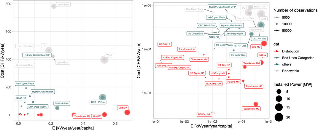
FIGURE 8. Energy system configuration of a neutral and independent Switzerland in 2050 under uncertainty. The x-axis displays the annual average power output by technology per capita $E[\frac{\mathrm{k}\mathrm{W}\mathrm{y}\mathrm{e}\mathrm{a}\mathrm{r}}{\mathrm{y}\mathrm{e}\mathrm{a}\mathrm{r}\mathrm{c}\mathrm{a}\mathrm{p}\mathrm{i}\mathrm{t}\mathrm{a}}]$, while the y-axis represents the cost per annual output $[\frac{\mathrm{C}\mathrm{H}\mathrm{F}}{\mathrm{k}\mathrm{W}\mathrm{y}\mathrm{e}\mathrm{a}\mathrm{r}}]$. (A) with a logarithmic scale, (B) corresponds to allowing us to distinguish the small size and cost technologies. The size of the outer bullet is proportional to the technology installed power, while the size of the inner bullet represents the capacity factor by plotting the average power output. The color scale categorizes the technologies in distribution, end-use categories, distribution, and renewables. The transparency scale corresponds to the logarithmic number of observations of the technology. Each centroid is displayed with horizontal and vertical error bars, displaying 95% quantiles of the centroid location.

The area of the generated rectangle between the origin and technology measures the annual investment per capita. The shape of the rectangles classifies technologies in base-load technologies for horizontal rectangles and backup technologies with vertical rectangles. Base-load technologies correspond to technologies with a high-capacity factor use.

The technologies have been categorized according to their use between renewable (harvesting), distribution, end-use, and other technologies. The categories are regrouped within Figure 8. Renewable energies are located in the high cost and energy area, necessary for harvesting the energy by converting primary energy potential into useful energy vectors. The sum of annually averaged renewable technologies converted specific energy per capita corresponds to 1.01 kW in comparison to the deployed averaged power of 4.73 kW, corresponding to an average capacity factor of 21.29%. This low-capacity factor is intrinsically due to the seasonal intermittence of the availability of resources². On the other side of the plot, energy infrastructure technologies create the baseline at a relatively low cost due to the existing infrastructure. Infrastructure technologies frame the bandwidth of all remaining technologies necessary to transport the harvested energy toward the end use and storage technologies at decentralized and centralized levels.

3.1.3 Uncertainty

The method has been adapted in order to observe the variation of the energy system configurations under the uncertainty, relying on the characterization and modeling of the grid infrastructure. The parameters characterizing the grid with their values and uniform distribution around their default value, with lower and upper bounds determined during their modeling, have been taken as input to the Sobol sequence³, generating a Monte-Carlo space and running the 50,000 iterations in the distribution of appearance of the energy system, represented through the error bars in Figure 8 and the grid reinforcement given in Table 3.

TABLE 3

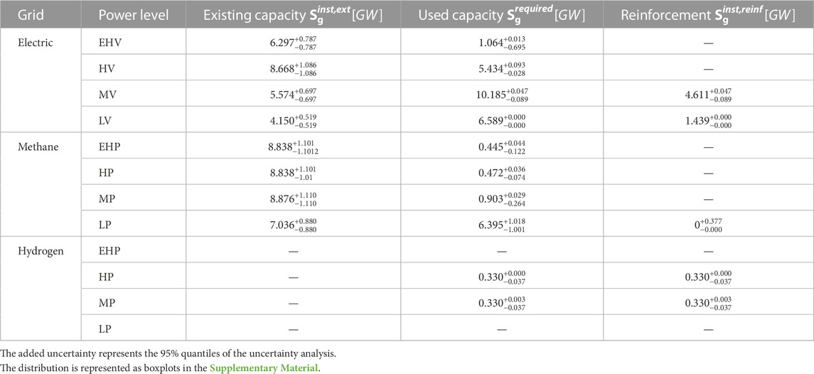
TABLE 3. Grid reinforcement based on existing capacities for the Swiss 2050 neutral and independent energy system configuration economic optimization under 50,000 Monte Carlo iterations.

Despite integrating the error bars, quasi non-existent variations within the main technologies can be observed. While the vertical axis depicts the cost of the technology per energy delivered, the error bar intrinsically shows only differences in the use of the technology, as their cost varies with the power installed, and therefore the ratio remains constant, unless the technology is used at a different amplitude throughout the year. Horizontal variations can be observed when a technology is installed at different capacities throughout the sensitivity analysis. The respective confidence intervals of the grid infrastructure can be observed in Table 2 and are depicted in Supplementary Figure S2. We can distinguish between three types of grid reinforcements: 1) the grids which, independently of the uncertainty analysis, are used at lower capacities at a unique peak, such as electric transmission grids (EHV and HV): 2) the grids which, independently of the uncertainty, will need the reinforcement of the grid (MV and LV electric grids); and 3) the grids which present two peaks, where the main peak is not reinforcing the grid capacity (95%), with the second peak being more spread out, following the uniform uncertainty of the existing grid. The last case does not induce additional investment and demonstrates the use of existing methane infrastructure under specific conditions (5%).

3.1.4 Grid reinforcement and use

In order to meet the demands at minimum cost, the model installs more efficient technologies in all sectors, which are powered by intermittent renewable technologies, mainly PV and wind. Due to the consumption phase shift, the converted primary energy has to be transported by networks, either directly to the consumer or in stocks. The energy carrier transport is constrained by the capacity of existing networks, which needs to be reinforced when the capacity is exceeded. This network reinforcement leads to increased costs. This sequence of relationships between demand fulfillment, primary energy conversion, transmission, storage, and network reinforcement is conducted simultaneously in optimization, minimizing the total costs. Table 3 lists the current capacity level based on the historical data of the 2020 system and the used grid power for the Swiss 2050 neutral and independent energy system configuration study. From this, it is possible to determine the grid reinforcement.

The existing capacity is based on the 2020 energy system configuration, a highly import-dependent energy system importing methane and electricity at extra high pressure and voltage.

The energy system 2050 is constrained to be energetically independent and CO₂-neutral, and a high share of renewable energy technologies are installed, corresponding to 15.4 GW PV and 20.0 GW wind deployment. The corresponding distribution grids were designed to satisfy the power load demand and decentralized production, which are not deployed in the current energy system. This additional production leads to reinforcement: the low-voltage grid needs to be able to absorb maximum solar energy during the summer months, while the medium-voltage grid is reinforced for maximum wind power production during winter.

While the methane grid is designed to meet the requirements of the 2020 gas-only import at EHP, the local biogas and synthetic methane production at lower levels needs to fulfill the existing capacity. Therefore, no reinforcement is needed in contrast to the hydrogen network. Furthermore, while no existing infrastructure could be identified in 2020, wood gasification generates 2.73 GWh of hydrogen, which is needed at a constant rate for fueling of coaches and trucks.

3.2 The role of grid reinforcement

After the definition of the economically optimal energy system and the respective grid reinforcement, it is possible to identify the role of reinforcement directly. Then, to measure its effects, the model is run for the identified electric grid level reinforcements (Table 3), varying from no reinforcement to the grid-specific optimal reinforcement.

Figure 9 represents the evolution of the energy system cost composition as a function of electricity LV (Figure 9A) and MV (Figure 9B) voltage reinforcement. On the secondary axis, the necessary storage capacity evolution is displayed. While the total cost decreases from 1220 CHF for no LV reinforcement and 1240 CHF for no MV reinforcement toward the optimum point of 1123 CHF with increasing reinforcement, the energy system composition adapts as a function of the available infrastructure.

FIGURE 9

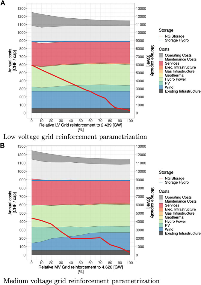
FIGURE 9. Evolution of energy system cost composition and storage capacities of the Swiss energy system according to grid reinforcement. Case study of the economic optimization of a neutral (no net emission) and independent (no imports) Swiss energy system in 2050 for a population of 10 million people. (A) represents the effect under the low voltage grid reinforcement parametrization. (B) represents the effect under the low voltage grid reinforcement parametrization.

The main investments are similar to those given in Figure 8; the energy harvesting technologies only use renewable energy. Wind, photovoltaics, and hydropower take a share between 48% and 51% of the total investment costs. Hydropower is installed at an almost constant rate, while wind and photovoltaics complement each other to reach approximately 300 CHF/cap, depending on the constrained grid reinforcement level. The existing LV infrastructure allows a deployment of 11.3 GW which is kept constant until a grid reinforcement of 10%, before linearly increasing to the economic optimum of 15.4 GW at an LV grid reinforcement of 2.439 GW (Figure 9A). Similar to the PV in LV reinforcement parametrization, the wind behaves similarly to the MV reinforcement. The MV grid reinforcement constrains wind power deployment. While with the existing infrastructure, 8.4 GW of wind can be installed, the MV grid reinforcement of 4.626 GW allows installing up to 20 GW of wind power, corresponding to the technical potential of Switzerland (Figure 9B).

The secondary axis of Figure 9 depicts the storage technology installed capacities. While hydro storage is used at the maximum possible capacity of 8.9 TWh independent of the grid reinforcements, methane storage eases the de-phasing of intermittency of renewable harvesting and consumption of final energies. Furthermore, methane storage is needed to store the output of wood gasification technologies. While the economic optimum is converting 5.2 TWh of wood, lower grid reinforcement leads to higher consumption of latter biomass, increasing to 9.7 TWh for no MV reinforcement and 15.3 TWh for no LV reinforcement. Later biomass consumption is visible in the operating costs in the same figures in the primal x-axis.

In addition to harvesting technologies, the distribution infrastructure takes minor shares in the cost composition. Due to the maximization of the use of the existing infrastructure (56 CHF/cap), the reinforcement of the electric networks dominates the grid costs compared to other infrastructure costs. While methane storage is the principal investment in the gas infrastructure with low-voltage grid reinforcement restraint (Figure 10A ), hydrogen infrastructure construction dominates the gas infrastructure reinforcement at low MV grid reinforcement $\le 20\%$ (Figure 10B). The gas infrastructure construction follows biomass conversion technologies. While wood is converted into methane through SNG gasification at low shares of grid reinforcements ($\le 50\%$ LV and $\le 40\%$ MV reinforcement), it is replaced by hydrogen production through hydrogen gasification at higher shares (Figures 10C, D).

FIGURE 10

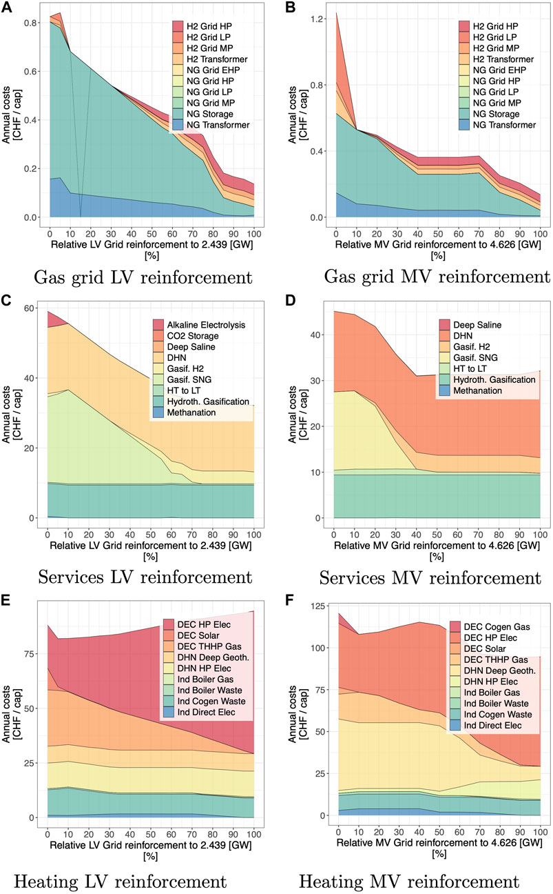
FIGURE 10. Evolution of energy system category cost composition of the 2050 Swiss energy system case study according to grid reinforcement. (A,C,E) LV reinforcement and (B,D,F) MV reinforcement.

Heating technologies follow the electrification of the energy system, dictated by the reinforcement (Figures 10E, F). While biomass gasification at low reinforcement levels compensates for the lack of electricity, the generated methane is used to power decentralized thermal gas heat pumps, decreasing linearly with the LV grid reinforcement. This decrease is compensated for by installing decentralized electric heat pumps powered by an increased share of photovoltaic panels. At low MV grid reinforcement, hydrogen production is used to power decentralized cogeneration technologies in fuel cells, heating, and powering the electricity demand of services and households. With increasing deployment of wind, the share of district heating is decreased, switching from DHN deep geothermal to DHN and decentralized electric heat pumps. Comparing (Figures 10E, F) shows the direct correlation between PV and decentralized electric heat pumps. With an increasing share of LV grid reinforcement, PV is installed, powering the decentralized heat pumps. In contrast, in the left figure (Figures 10E), the decentralized heat pump share is almost constant, similar to the amount of PV deployed. This behavior leads to a decrease of the heating costs by 23.7% with the reinforcement of MV but an increase by 15.1% for the LV reinforcement.

3.3 The interplay of wind and photovoltaics

In the grid reinforcement results, we showed how the modeling constraint reaches the ideal PV–wind ratio for this case study. The effect of the interplay between the deployment of PV and wind is questioned. In order to answer this question, the deployment of PV is modeled from 0 to its maximum potential of 50 GW and applied to the previously described use case.

Figure 11 represents the cost composition and storage capacities under the parameterized deployment of photovoltaic panels from 0 to 50 GW. The economic optimum is visible at 30.8% installed capacity, corresponding to the previously identified amount of 15.4 GW of PV panels. Reducing this amount leads to an increase in the operating costs due to a higher share of consumed wood (10.0 TWh compared to 5.2 TWh at the optimum and 3.4 TWh at full PV deployment).

FIGURE 11

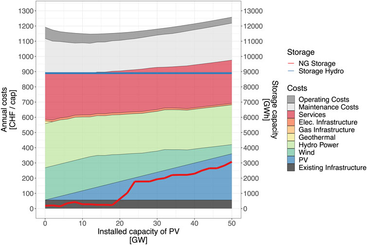
FIGURE 11. Evolution of investments and storage capacity of the Swiss energy system according to PV penetration in 2050. Case study of the economic optimization of a neutral (no net emission) and independent (no imports) Swiss energy system in 2050.

The wind is deployed at maximum capacity until PV reaches 16 GW. After this inflection point, the wind is reduced and compensates for the increased share of PV in the energy mix, ending at 5.6 GW of wind at the PV maximum potential.

Similar to the previously discussed grid reinforcement, hydro storage is used at its maximum capacity of 8.90 TWh, independent of PV deployment. Methane storage fluctuates according to the PV parametrization, where 0.85 TWh is installed at no PV before decreasing to 0.34 TWh between 2 and 18 GW, corresponding to the inflection point of wind. With decreasing wind share, the methane storage capacity is increased to 3.13 TWh, as observed previously with the MV grid reinforcement.

Increasing the PV share in the energy system leads to LV infrastructure reinforcement (Figure 12A). While the need for transformers increases with the electrification of the energy system, MV reinforcement decreases with the decreasing quantity of wind installed. The minimum grid reinforcement locates at no installed photovoltaics, where the system switches toward compensation by biomass. The electric infrastructure drop is compensated for by installing gas infrastructure (Figure 12B). In addition to the hydrogen infrastructure construction, methane storage takes the highest share of the gas infrastructure costs. Methane storage behaves inversely to the hydrogen infrastructure construction, as the highest shares of hydrogen are observed at the lowest methane storage investments.

FIGURE 12

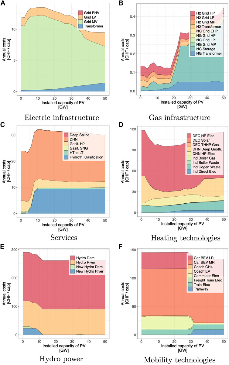
FIGURE 12. Evolution of investments according to PV penetration of the 2050 independent and neutral Swiss energy system case study. Each subfigure represents the investments in a specific sector.

The energy system configuration between 0 and 2.5 GW PV is characterized by lower electrification of the energy system compared to the optimum (−15.8 TWh). The compensation is achieved through three energy resources: 1) different use of the biomass resource, 2) deep geothermal district heating and electricity generation, and 3) installation of new hydropower plants.

Additional biomass is used to compensate for the lack of electricity. While wet biomass and waste are converted in the same way as at the optimum, wood consumption is increased (+5.1 TWh) in order to generate hydrogen (+0.5 TWh) and methane (+3.3 TWh) through gasification (Figure 12C).

The lack of electricity leads to installing alternative heating technologies (Figure 12D). While industrial process heat is generated with biomass (waste and synthetic methane) rather than direct electric heat, district heating is achieved by deep geothermal heating (+15.1 TWh). At the decentralized level, the leading heating technology remains at electric heat pumps (13.8 GW), which are complemented by 2.3 GW of thermal gas heat pumps.

Hydro dams are reinforced by 0.44 GW in addition to 0.85 GW of new hydro river plants, generating 4.5 TWh of additional electricity (Figure 12E). While EHV electricity generated by the hydro dams is converted to satisfy heating and direct electricity demands, new HV hydro river electricity is directly correlated to public rail mobility technologies, installing commuters rather than tramway trolleys (Figure 12F).

Between 2.5 GW and the optimum point of 15.7 GW of PV deployment, the wind is still used at the maximum potential of 20 GW. Within this area, biomass consumption is kept at a constant rate. At the same time, the biomass conversion switches from SNG gasification to hydrothermal gasification, combining heat and power. This direct gas usage leads to lower gas transportation and methane storage necessities.

While continuously increasing the share of PV, electrification of the low-temperature heating technologies increases too $(+34.6\frac{\%}{{\mathrm{G}\mathrm{W}}^{{\mathrm{P}\mathrm{V}}^{+}}})$. Decentralized and district-heating electric heat pumps are deployed, replacing deep geothermal and gas-powered heating technologies. The energy system’s electrification allows for reducing the amount of hydropower to 0.

Once the optimum PV deployment point is passed, increasing PV leads to a decrease in wind capacity installation $(-0.235\frac{{\mathrm{G}\mathrm{W}}^{\mathrm{W}\mathrm{i}\mathrm{n}\mathrm{d}}}{{\mathrm{G}\mathrm{W}}^{{\mathrm{P}\mathrm{V}}^{+}}})$. Increasing PV production leads to increasing LV grid costs, while reducing wind decreases the MV grid reinforcement. While at the optimum point the ratio of wind and PV allowed to power the respective technologies at the most efficient levels, moving away from this optimal ratio leads to additional conversion in voltage levels, leading to increasing transformer costs.

Another effect of increasing the share of PV to the detriment of wind leads to the de-phasing of seasonal production maximum in summer and consumption with the highest demands in winter. The increased primary energy demand $(+0.155\frac{\mathrm{T}\mathrm{W}\mathrm{h}}{{\mathrm{G}\mathrm{W}}^{{\mathrm{P}\mathrm{V}}^{+}}})$ therefore requires methane storage $(+82\frac{\mathrm{G}\mathrm{W}\mathrm{h}}{{\mathrm{G}\mathrm{W}}^{{\mathrm{P}\mathrm{V}}^{+}}})$ to overcome the seasonal mismatch in heating. While the gas resource is used for cogeneration, reducing the heating efficiency, additional district heating deep geothermal plants compensate for the lack of heating.

With increasing electrifying of the energy system, sectors are independent of the seasonal shift for electric technologies, such as industrial process heat generation or electric trains.

4 Discussion

In this study, the presented modeling framework allows the comparison and characterization of different infrastructure technologies on the same level of detail, enabling the integration of different constraining parameters regarding time and geographic resolution differences in linear modeling frameworks. Furthermore, the linear modeling approach has been validated through historical data of the Switzerland 2020 energy system before being applied to the 2050 Swiss neutral and independent energy system.

Proceeding to economic optimization on the latter case study shows the maximization of usage of existing infrastructure, while the electrification of the energy system with the deployment of high shares of PV and wind leads to the necessity of electric grid reinforcement.

The optimal mix sees methane as a heating vector for industrial purposes and hydrogen as a long-distance public road transport fuel. Limiting the reinforcement of electric grids leads to lower electrification in harvesting technologies, which is compensated for by biomass conversion, using existing gas infrastructure and up to 6 TWh of methane storage.

Seasonal storage is achieved at the highest possible density at a centralized level. While electric storage is achieved by using the maximum existing infrastructure at the EHV level with hydro dams at 8.9 TWh, the gas storage is installed at the EHP grid using methane storage in the range between 0.6 and 6 TWh.

Limiting grid reinforcement leads to constraints on the electrification of the system, limiting the deployment of wind and PV. The energy system turns toward other energy resources, such as electric resources at the transmission level (geothermal and new hydro installations) and higher consumption of biomass, using the existing methane infrastructure, increasing the total system cost by up to 16%.

The selection of less efficient, more cost-intensive technologies and the use of biomass further dephase energy resource conversion and consumption. The seasonal shift is compensated for by installing up to 5.8 TWh seasonal methane storage. Primary energy conversion directly affects the deployment of end-use technologies. Lower electrification leads to alternative heating and mobility technologies, switching to gas-powered technologies.

PV and wind complement each other ideally in order to smooth seasonal differences at a power ratio of 4:5.

Decreasing this ratio necessitates complementing the lack of primary energy in summer with biomass gasification, hydropower reinforcement, and geothermal power. Methane storage becomes necessary as soon as other electric resources and the transition of low-temperature heating to gas technologies cannot compensate for the missing share of deployed PV.

Like the renewable electric resources, biomass use is limited within the model (Li et al., 2020), where the potential for energetic use has been estimated by Oliver Thees (2017). Therefore, the existing biomass potential is sufficient to cover the extrinsic variation of renewable electricity sources.

Increasing the ratio leads to the deployment of higher shares of PV and less wind. Therefore, low wind electricity production in winter needs to be compensated for by deploying more PV, increasing the annual primary energy conversion of PV and wind compared to the optimum point.

The high share of PV (LV) and wind (MV) deployment leads to investments in reinforcing the electric distribution grid. However, the transmission grid capacity is not reached and therefore does not need additional reinforcement. The existing methane grid is used as a back-up for transporting the gas necessary in seasonal storage from perturbations, using up to the existing grid capacity limits. Hydrogen is used as a freight mobility vector only at minor shares.

This study considers a geographically and temporally averaged model. The effect of the temporal resolutions on energy system modeling has been assessed (Limpens et al., 2019) by adapting the monthly EnergyScope model to an hourly resolution and by (Schnidrig et al., 2020) assessing the impact of mobility technologies on the energy system at monthly and hourly aggregation. No significant differences in the installation of seasonal technologies have been observed in both studies. The limitations have been identified by observing the installation of inter- and intra-daily storage technologies within the hourly model, which affects the total cost composition with additional investments and also the seasonal technologies in a negligible manner. The monthly aggregated model, therefore, is not depicting the installation of daily technologies such as batteries, water tanks, and vehicle-to-grid.

Spatial aggregation leads to the assumption that all production and consumption are made in one spot, while the electrons and gas molecules are traveling on an averaged grid according to the respective production or consumption power level, which was based on a mainly centralized production case study.

This assumption does not consider the role of future decentralization of the energy system, where harvesting, conversion, storage, and consumption are made remotely, not connected to the grid, such as in smart districts or buildings. This limitation leads to a possible overestimation of distribution networks.

Another limitation of this assumption is not considering further centralization of production and the necessity of energy transmission through bottlenecks. Seasonal storage has been identified as having high-density levels, existing at centralized locations currently. The transition from consumer to prosumer leads to new operation strategies of the grid, differing from the existing transmission network operation, leading to possible bottlenecks. This limitation can be weakened due to the characteristics of the case study, where Switzerland’s infrastructure was operated and designed to allow the transition of electricity and methane within the European energy grid. Therefore, existing infrastructure provides centralized production at differing geographic levels of the consumption nodes.

The application of geographic aggregation leads to uncertainty in the distribution network. While assessing this uncertainty within the Monte-Carlo sensitivity analysis, we conclude that the uncertainty related to the values does not significantly influence the decisions taken by the global system. The role of decentralization and the effect of geographic distribution are subject to a future publication in redaction.

5 Conclusion

For the first time, we compared different energy vector transportation grids at a common level and integrated them into a global energy system model. The capacity and length of the distribution networks characterize the infrastructure. This approach allows scientists in future studies to compare different energy transportation infrastructures, despite their seemingly different nature.

The model shows that it is possible to reach CO₂-neutral and energy-independent energy system in 2050 by installing efficient technologies in all sectors powered by intermittent renewable technologies, mainly wind and PV. However, the transportation of those energy carriers is limited by the capacity of the existing grids, which needs to be reinforced when capacity is exceeded, which is observed in the MV and LV grids due to the heavy deployment of wind and PV. The modeling condition achieves the ideal PV-to-wind ratio for this case study. The economic optimum is seen at 30.8% installed capacity, corresponding to the 15.4 GW of PV panels identified earlier. A reduction in this amount results in higher operating costs due to a higher proportion of wood consumed. Wind is used at its maximum capacity until PV reaches 16 GW.

The role of grid reinforcements and their influence on the energy system composition is assessed in this study. Limiting the electric grid reinforcement on one level leads to the lower deployment of either PV (LV) or wind (MV). It, therefore, leads to higher de-phasing between production and consumption, thus increasing the need for seasonal storage, which is achieved using existing gas transmission infrastructure and methane storage (up to 6 TWh).

We, therefore, demonstrate the necessity to account for existing infrastructure energy systems optimization, as all simulations run to maximize the utilization of existing infrastructure. The choices in deploying and developing new infrastructure for today's energy systems must be made carefully with a long-term perspective, as the next generations will pay for rash decisions.

Data availability statement

The original contributions presented in the study are publicly available. This data can be found here: https://gitlab.com/ipese/on-the-role-of-energy-infrastructure-in-the-energy-transition.

Author contributions

JS contributed to the conception and design of the study, modeling, result analysis, and redaction. FM and MM contributed to study conceptualization. YC and RC contributed to validation and review. All authors contributed to manuscript revision, read, and approved the submitted version.

Funding

The authors acknowledge the financial support from the Energy Center EPFL (CEN) Lausanne, Switzerland, within the EnergyScope 2.0 project (GDB 19349) of the Swiss Federal Office of Energy funding. Open access funding by École Polytechnique Fédérale de Lausanne. The authors acknowledge the financial support from the Swiss Federal Office of Energy under grant Sl/502039-01 and from the Association of the Swiss Gas Industry VSG under grant FOGA-0305.

Conflict of interest

The authors declare that the research was conducted in the absence of any commercial or financial relationships that could be construed as a potential conflict of interest.

Publisher’s note

All claims expressed in this article are solely those of the authors and do not necessarily represent those of their affiliated organizations, or those of the publisher, the editors, and the reviewers. Any product that may be evaluated in this article, or claim that may be made by its manufacturer, is not guaranteed or endorsed by the publisher.

Supplementary material

The Supplementary Material for this article can be found online at: https://www.frontiersin.org/articles/10.3389/fenrg.2023.1164813/full#supplementary-material

Abbreviations

EHP, extra high pressure; EPFL, École Polytechnique Fédérale de Lausanne; EHV, extra high voltage; HP, high pressure; HV, high voltage; IPCC, International Panel on Climate Change; LP, low pressure; LV, low voltage; MP, medium pressure; MV, medium voltage; NG, methane (equivalent to methane); PV, photovoltaic panels; RPE, renewable primary energy; SFOE, Swiss Federal Office of Energy; SOEC, solid oxide electrolyzer cell; SoS, security of supply.

Footnotes

¹For mass-based technologies, the sizing equivalent is [kt], person mobility [Mpkm], and freight mobility [Mtkm].

²The energy systems centroid seasonal variation is depicted in Supplementary Material.

³The uncertainty distribution of the parameters considered is visible in Supplementary Material in the respective section.

References

Abrell, J., Eser, P., Garrison, J. B., Savelsberg, J., and Weigt, H. (2019). Integrating economic and engineering models for future electricity market evaluation: A Swiss case study. Energy Strategy Rev. 25, 86–106. doi:10.1016/j.esr.2019.04.003

CrossRef Full Text | Google Scholar

Antenucci, A., Crespo del Granado, P., Gjorgiev, B., and Sansavini, G. (2019). Can models for long-term decarbonization policies guarantee security of power supply? A perspective from gas and power sector coupling. Energy Strategy Rev. 26, 100410. doi:10.1016/j.esr.2019.100410

CrossRef Full Text | Google Scholar

Bartlett, S., Dujardin, J., Kahl, A., Kruyt, B., Manso, P., and Lehning, M. (2018). Charting the course: A possible route to a fully renewable Swiss power system. Energy 163, 942–955. doi:10.1016/j.energy.2018.08.018

CrossRef Full Text | Google Scholar

Becker, S., Frew, B. A., Andresen, G. B., Zeyer, T., Schramm, S., Greiner, M., et al. (2014). Features of a fully renewable US electricity system: Optimized mixes of wind and solar PV and transmission grid extensions. Energy 72, 443–458. doi:10.1016/j.energy.2014.05.067

CrossRef Full Text | Google Scholar

Capellán-Pérez, I., de Castro, C., and Miguel González, L. J. (2019). Dynamic Energy Return on Energy Investment (EROI) and material requirements in scenarios of global transition to renewable energies. Energy Strategy Rev. 26, 100399. doi:10.1016/j.esr.2019.100399

CrossRef Full Text | Google Scholar

Capros, P.E3MLab, ICCS, NTUA (2013). Primes model. Model description. Athens: National Technical University of Athens.

Google Scholar

Capros, P.E3MLab, ICCS, NTUA (2010). Prometheus model documentation. Model description, 1. Athens: National Technical University of Athens.

Google Scholar

Capros, P., and Siskos, P.E3MLab, ICCS, NTUA (2011). PRIMES-TREMOVE transport model. Model description, 3. Athens: National Technical University of Athens.

Google Scholar

Day, C., Hobbs, B., and Pang, J.-S. (2002). Oligopolistic competition in power networks: A conjectured supply function approach. IEEE Trans. Power Syst. 17, 597–607. doi:10.1109/tpwrs.2002.800900

CrossRef Full Text | Google Scholar

de Nooij, M., Koopmans, C., and Bijvoet, C. (2007). The value of supply security: The costs of power interruptions: Economic input for damage reduction and investment in networks. Energy Econ. 29, 277–295. doi:10.1016/j.eneco.2006.05.022

CrossRef Full Text | Google Scholar

Dias, L. P., Simões, S., Gouveia, J. P., and Seixas, J. (2019). City energy modelling - optimising local low carbon transitions with household budget constraints. Energy Strategy Rev. 26, 100387. doi:10.1016/j.esr.2019.100387

CrossRef Full Text | Google Scholar

Dujardin, J., Kahl, A., and Lehning, M. (2021). Synergistic optimization of renewable energy installations through evolution strategy. Environ. Res. Lett. 16, 064016. doi:10.1088/1748-9326/abfc75

CrossRef Full Text | Google Scholar

Eidgenössische Elektrizitätskommission ElCom (2021). Tätigkeitsbericht der Elcom 2020. Tech. Rep., eidgenössische elektrizitätskommission ElCom. Bern.

Google Scholar

Federal Statistical Office (2017). Gebäude nach Heizsystem und Energieträger.

Google Scholar

Fishbone, L. G., and Abilock, H. (1981). Markal, a linear-programming model for energy systems analysis: Technical description of the bnl version. Int. J. Energy Res. 5, 353–375. doi:10.1002/er.4440050406

CrossRef Full Text | Google Scholar

Gabriel, S. A., Kydes, A. S., and Whitman, P. (2001). The national energy modeling system: A large-scale energy-economic equilibrium model. Operations Res. 49, 14–25. doi:10.1287/opre.49.1.14.11195

CrossRef Full Text | Google Scholar

Garrison, J. B., Demiray, T., Abrell, J., Savelsberg, J., Weigt, H., and Schaffner, C. (2018). “Combining investment, dispatch, and security models - an assessment of future electricity market options for Switzerland,” in 2018 15th International Conference on the European Energy Market ( Lodz, Poland: EEM), 1–6. doi:10.1109/EEM.2018.8469895

CrossRef Full Text | Google Scholar

Gholizadeh, N., Vahid-Pakdel, M. J., and Mohammadi-ivatloo, B. (2019). Enhancement of demand supply’s security using power to gas technology in networked energy hubs. Int. J. Electr. Power & Energy Syst. 109, 83–94. doi:10.1016/j.ijepes.2019.01.047

CrossRef Full Text | Google Scholar

Gupta, R. K., Sossan, F., Le Boudec, J.-Y., and Paolone, M. (2021b). Compound admittance matrix estimation of three-phase untransposed power distribution grids using synchrophasor measurements. IEEE Trans. Instrum. Meas. 70, 1–13. doi:10.1109/tim.2021.3092063

PubMed Abstract | CrossRef Full Text | Google Scholar

Gupta, R., Sossan, F., and Paolone, M. (2021a). Countrywide PV hosting capacity and energy storage requirements for distribution networks: The case of Switzerland. Appl. Energy 281, 116010. doi:10.1016/j.apenergy.2020.116010

CrossRef Full Text | Google Scholar

Hampp, J., Düren, M., and Brown, T. (2023). Import options for chemical energy carriers from renewable sources to Germany. PLOS ONE 18, e0262340. doi:10.1371/journal.pone.0281380

PubMed Abstract | CrossRef Full Text | Google Scholar

Hörsch, J., Hofmann, F., Schlachtberger, D., and Brown, T. (2018). PyPSA-Eur: An open optimisation model of the European transmission system. Energy Strategy Rev. 22, 207–215. doi:10.1016/j.esr.2018.08.012

CrossRef Full Text | Google Scholar

Howell, G. W., and Weathers, T. M. (1970). Aerospace fluid component designers’ handbook. Volume I, revision D. Tech. rep. Redondo Beach, CA: TRW SYSTEMS GROUP REDONDO BEACH CA.

Google Scholar

Howells, M., Rogner, H., Strachan, N., Heaps, C., Huntington, H., Kypreos, S., et al. (2011). OSeMOSYS: The open source energy modeling system. Energy Policy 39, 5850–5870. doi:10.1016/j.enpol.2011.06.033

CrossRef Full Text | Google Scholar

Jacobson, M. Z., Delucchi, M. A., Cameron, M. A., and Frew, B. A. (2015). Low-cost solution to the grid reliability problem with 100% penetration of intermittent wind, water, and solar for all purposes. Proc. Natl. Acad. Sci. 112, 15060–15065. doi:10.1073/pnas.1510028112

PubMed Abstract | CrossRef Full Text | Google Scholar

Jensen, I. G., Wiese, F., Bramstoft, R., and Münster, M. (2020). Potential role of renewable gas in the transition of electricity and district heating systems. Energy Strategy Rev. 27, 100446. doi:10.1016/j.esr.2019.100446

CrossRef Full Text | Google Scholar

Kayal, P., and Chanda, C. K. (2015). Optimal mix of solar and wind distributed generations considering performance improvement of electrical distribution network. Renew. Energy 75, 173–186. doi:10.1016/j.renene.2014.10.003

CrossRef Full Text | Google Scholar

Kost, M. (2021). Gesamtenergiestatistik 2020. Tech. Rep. Bern: BFE, 10537.

Google Scholar

Lapillonne, B. (1978). Medee 2: A model for long-term energy demand evaluation. Tech. rep. Laxenburg, Austria: International Institue for Applied Systems Analysis.

Google Scholar

Leuthold, F. U., Weigt, H., and von Hirschhausen, C. (2012). A large-scale spatial optimization model of the European electricity market. Netw. Spatial Econ. 12, 75–107. doi:10.1007/s11067-010-9148-1

CrossRef Full Text | Google Scholar

Li, A., and Zheng, H. (2021). Energy security and sustainable design of urban systems based on ecological network analysis. Ecol. Indic. 129, 107903. doi:10.1016/j.ecolind.2021.107903

CrossRef Full Text | Google Scholar

Li, X., Damartzis, T., Stadler, Z., Moret, S., Meier, B., Friedl, M., et al. (2020). Decarbonization in complex energy systems: A study on the feasibility of carbon neutrality for Switzerland in 2050. Front. Energy Res. 8, 549615. doi:10.3389/fenrg.2020.549615

CrossRef Full Text | Google Scholar

Limpens, G., Moret, S., Jeanmart, H., and Maréchal, F. (2019). EnergyScope td: A novel open-source model for regional energy systems. Appl. Energy 255, 113729. doi:10.1016/j.apenergy.2019.113729

CrossRef Full Text | Google Scholar

Manne, A. S., and Wene, C. O. (1992). MARKAL-MACRO: A linked model for energy-economy analysis. Goeteborg: Chalmers Univ. of Tech. doi:10.2172/10131857

CrossRef Full Text | Google Scholar

Moret, S., Codina Gironès, V., Bierlaire, M., and Maréchal, F. (2017). Characterization of input uncertainties in strategic energy planning models. Appl. Energy 202, 597–617. doi:10.1016/j.apenergy.2017.05.106

CrossRef Full Text | Google Scholar

Morokoff, W. J., and Caflisch, R. E. (1995). Quasi-Monte Carlo integration. J. Comput. Phys. 122, 218–230. doi:10.1006/jcph.1995.1209

CrossRef Full Text | Google Scholar

Neelakanta, P., and Arsali, M. (1999). Integrated resource planning using segmentation method based dynamic programming. IEEE Trans. Power Syst. 14, 375–385. doi:10.1109/59.744558

CrossRef Full Text | Google Scholar

Thees, O., Burg, V., Erni, M., Bowman, G., and Lemm, R. (2017). Biomassepotenziale der Schweiz für die energetische Nutzung. Ergebnisse des Schweizerischen Energiekompetenzzentrums SCCER BIOSWEET. WSL Berichte. Birmensdorf: Eidg. Forschungsanstalt fr Wald, Schnee und Landschaft WSL, 299

Google Scholar

Papadopoulos, C., Johnson, R., and Valdebenito, F. (2000). PLEXOS® integrated energy modelling around the globe. Tech. rep. Australie: Energy Exemplar Pty Ltd, Prospect.

Google Scholar

Pörtner, H.-O., Roberts, D. C., Tignor, M. M. B., Poloczanska, E., Mintenbeck, K., Alegría, A., et al. (2022). Climate change 2022: Impacts, adaptation, and vulnerability. Tech. Rep. Switzerland: IPCC, 6.

Google Scholar

Reza Norouzi, M., Ahmadi, A., Esmaeel Nezhad, A., and Ghaedi, A. (2014). Mixed integer programming of multi-objective security-constrained hydro/thermal unit commitment. Renew. Sustain. Energy Rev. 29, 911–923. doi:10.1016/j.rser.2013.09.020

CrossRef Full Text | Google Scholar

Richstein, J. (2022). Openmod - open energy modelling initiative.

Google Scholar

Schlecht, I., and Weigt, H. (2014). Swissmod - a model of the Swiss electricity market. SSRN Electron. J. 2014. doi:10.2139/ssrn.2446807

CrossRef Full Text | Google Scholar

Schmid, D., Korkmaz, P., Blesl, M., Fahl, U., and Friedrich, R. (2019). Analyzing transformation pathways to a sustainable European energy system—internalization of health damage costs caused by air pollution. Energy Strategy Rev. 26, 100417. doi:10.1016/j.esr.2019.100417

CrossRef Full Text | Google Scholar

Schnidrig, J., Nguyen, T.-V., Li, X., and Marechal, F. (2021). “A modelling framework for assessing the impact of green mobility technologies on energy systems,” in Proceedings of ECOS 2021. Editor F. Marechal (Taormina, ITALY: ECOS 2021 Local Organizing Committee), 13.

Google Scholar

Schnidrig, J., Nguyen, T.-V., and Marechal, F. (2020). Assessment of green mobility scenarios on European energy systems.

Google Scholar

Schrattenholzer, L. (1981). The energy supply model MESSAGE. Tech. rep. Laxenburg, Austria: IIASA.

Google Scholar

Shobole, A. A., and Wadi, M. (2021). Multiagent systems application for the smart grid protection. Renew. Sustain. Energy Rev. 149, 111352. doi:10.1016/j.rser.2021.111352

CrossRef Full Text | Google Scholar

Siala, K., and Mahfouz, M. Y. (2019). Impact of the choice of regions on energy system models. Energy Strategy Rev. 25, 75–85. doi:10.1016/j.esr.2019.100362

CrossRef Full Text | Google Scholar

Sobol’, I. M. (1969). On the distribution of points in a cube and the approximate evaluation of integrals. U.S.S.R. Comput. Math. Math. Phys. 7, 86–112. doi:10.1016/0041-5553(67)90144-9

CrossRef Full Text | Google Scholar

Stadler, D. P., and Maréchal, F. (2020). The integrative role of natural gas in the energy transition of Switzerland. Tech. rep. Gaznat, Lausanne, Switzerland.

Google Scholar

Staffell, I., Scamman, D., Abad, A. V., Balcombe, P., Dodds, P. E., Ekins, P., et al. (2019). The role of hydrogen and fuel cells in the global energy system. Energy & Environ. Sci. 12, 463–491. doi:10.1039/c8ee01157e

CrossRef Full Text | Google Scholar

Swiss Geoportal (2019). Registre des bâtiments et des logements. Wabern: Office fédéral de la statistique.

Google Scholar

Swissgas (2018). Schweizerisches erdgastransportnetz 2018.

Google Scholar

Swissgrid (2020). Grid levels. Available at: https://www.swissgrid.ch/en/home/operation/power-grid/grid-levels.html.

Google Scholar

Verband der Schweizerischen Gasindustrie VSG (2020). Das Jahr in zahlen. tech. Rep., gazenergie, Zürich, Switzerland.

Google Scholar

Welsch, M., Howells, M., Hesamzadeh, M. R., Gallachóir, B. Ó., Deane, P., Strachan, N., et al. (2015). Supporting security and adequacy in future energy systems: The need to enhance long-term energy system models to better treat issues related to variability. Int. J. Energy Res. 39, 377–396. doi:10.1002/er.3250

CrossRef Full Text | Google Scholar

Witek, M., and Uilhoorn, F. E. (2021). Influence of gas transmission network failure on security of supply. J. Nat. Gas Sci. Eng. 90, 103877. doi:10.1016/j.jngse.2021.103877

CrossRef Full Text | Google Scholar

Zeljko, M., Aunedi, M., Slipac, G., and Jakšić, D. (2020). Applications of wien automatic system planning (WASP) model to non-standard power system expansion problems. Energies 13, 1392. doi:10.3390/en13061392

CrossRef Full Text | Google Scholar

Zhou, Y., Wu, J., and Long, C. (2018). Evaluation of peer-to-peer energy sharing mechanisms based on a multiagent simulation framework. Appl. Energy 222, 993–1022. doi:10.1016/j.apenergy.2018.02.089

CrossRef Full Text | Google Scholar

Nomenclature