Modelling and onsite testing on dynamic thermal responses of built environment in passive solar rooms on Tibetan plateau

1 Introduction

As global climate change has been drawing increasing concern, building and construction industry are caching growing attentions, since they accounts for dominant energy usage (Cao et al., 2023) and greenhouse gas emissions (Christopher et al., 2023), leading to accelerating global warming (Tirelli and Besana, 2023). In China, buildings are responsible for over 30% primary energy consumptions. And therein Moreover, about 60% can be attributed to building service systems, such space cooling and heating (Zhang and Luo, 2023).

With the rapid economic and technological development, regions like western Sichuan and the Qinghai-Tibet Plateau have attracted widespread attention due to their abundant solar energy resources (Zhang et al., 2020). Additionally, owing to the significant heating demand throughout the year, researchers have designed and studied various heating systems considering solar energy. For instance (Qiang et al., 2023), investigated solar-assisted heat pump systems, while (Li et al., 2023) utilized K-means algorithm combined with air-source heat pump to analyze the active heating behavior characteristics of residents living in high-altitude areas, suggesting a potential correlation between these behaviors and the improvement of energy efficiency (Chen et al., 2022). proposed eight potential solar energy system schemes for reducing building energy consumption in the Qinghai-Tibet Plateau, establishing optimization models for the lifecycle costs of each solar energy system. They analyzed the short-term dynamic operation performance, energy conservation, economics, and carbon emission reduction of the systems, presenting a comprehensive solar energy integration system with the best performance. Furthermore (Liu et al., 2022), researched the optimal capacity ratio of solar heating systems for office buildings in the Qinghai-Tibet Plateau and developed a SHS capacity matching optimization model with a minimum lifecycle cost as the objective function and multi-source complementary heating system (Liu Y. et al., 2021) are designed and investigated in those areas. However, solar energy exhibits characteristics such as uneven spatial-temporal distribution, strong intermittency, low efficiency, and high cost. Accurate prediction of dynamic thermal loads is crucial for the application of these systems.

Few studies focused During recent decades, more than 100 building energy simulation software programs (BLAST, DOE-2, EnergyPlus, TRNSYS, DeST, ESP-r) or self-programming based on energy conservation have been primarily utilized worldwide (Ren et al., 2023). These software solutions encompass a range of functionalities, including building dynamic load simulation and HVAC equipment system simulation. Notably, the heart of these software tools lies in the simulation of cooling and heating loads. Additionally, system simulation is a crucial component, focusing on replicating the control processes of air conditioning and heating system components. This simulation stage plays a pivotal role in bridging the gap between dynamic load simulation and energy consumption prediction. In recent years, scholars and engineering technicians have already utilized software to conduct scientific research, as well as to assist in the design and optimization of complex air conditioning and heating projects. In recent years, EnergyPlus, as the most widely used software globally, has been extensively employed (Liu S. M. et al., 2021). utilized EnergyPlus software to simulate the performance of different ventilation modes in residential buildings and the energy consumption of ventilation in typical apartments, proposing appropriate residential ventilation modes, particle filtration, and heat recovery usage strategies (Khan et al., 2022). employed EnergyPlus software to simulate the enhancement of energy performance in Pakistani residential buildings using PCM materials (Ng et al., 2021). utilized EnergyPlus software to simulate the impact of building infiltration on building energy consumption in commercial buildings, emphasizing the need to fully consider infiltration effects on HVAC energy use in building modeling (Emil and Diab, 2021). analyzed the potential for zero-energy renovation of educational buildings in Egypt using EnergyPlus software (Qi and Wang, 2023). investigated the optimization potential of building surface reflectance using EnergyPlus software (Al-janabi et al., 2019). compared the capabilities of EnergyPlus and IES for discussing the differences in design processes and results of different energy modeling software. While a large body of research has to some extent confirmed its effectiveness, most of these studies and applications are situated in plains or low-altitude areas, making them unsuitable for high-altitude regions. Furthermore, in indoor thermal environment research, scholars currently primarily employ field measurements (Huang and Kang, 2021) to study the impact of solar radiation on indoor thermal comfort and the occupants’ response to solar radiation in the indoor environment. Survey-based studies (Thapa, 2020) propose new comfort zones for regions with similar cold climates based on the results of field surveys on thermal comfort. Numerical simulations (Wang et al., 2023) using the jet flow model propose a coupled oxygen-thermal jet flow equation for creating a good indoor thermal environment and addressing low oxygen pressure in high-altitude regions. Additionally, studies employing computer modeling methods (Alwetaishi et al., 2020) investigated the influence of heat quantity and direction on the thermal performance levels of Shubra and Boqri palaces (Liu et al., 2019). studied the impact of window-to-wall ratio and daylighting depth on the thermal comfort of passive solar houses through computer modeling. Traditional thermal modeling methods are primarily based on more common and lower-altitude regions, overlooking the unique climatic characteristics of high-altitude areas. High-altitude regions often exhibit characteristics such as low atmospheric pressure, large diurnal temperature variations, low sky background temperature, and intense solar radiation. The low atmospheric pressure affects airflow velocity, thereby influencing the indoor thermal environment of buildings. Temperature variations impact the thermal insulation of buildings, while solar radiation affects the source of indoor temperatures, resulting in indoor thermal environments distinct from those in plains areas. The application of traditional thermal modeling methods may lead to differences or errors in building load prediction and energy efficiency assessment.

Most of the studies mentioned above are conducted in non-high-altitude areas, and there is currently limited research on continuous prediction models for indoor thermal environments in high-altitude mountainous regions. The primary objective of this research is to devise a methodology capable of predicting indoor thermal environment and heat consumption in passive buildings situated within alpine high-altitude regions. To fulfill this aim, a comprehensive approach was adopted. The initial step involved the creation of a mathematical model for a prototypical building, anchored in the principles of energy conservation. Subsequently, actual model buildings were erected, facilitating on-site data collection in a representative locale. These measurements encompassed variations in indoor air temperature under diverse scenarios, including natural conditions and heating scenarios, considering factors such as window-to-wall ratios (WWR), architectural orientations, and heat transfer coefficients. Ultimately, the integrity of the mathematical model was ascertained through rigorous validation utilizing the acquired empirical data.

2 Methodology and modelling

2.1 Indoor thermal environment

For modelling simplification, a typical case room is chosen with certain envelope structures (Figure 1). It's worth noting that even when there’s no solar radiation, thermal conductivity stemming from temperature differences within the non-transparent enclosure remains a factor. Applying the principle of energy conservation, the lumped parameter method was adopted to analyze the heat transfer of the room. Some basic considerations and assumptions are as follows.

(1) Uniform distribution for solar radiation on external building surfaces.

(2) Regardless of air leakage between rooms and thermal contact resistance between wall layers.

(3) Solar radiation is absorbed by both the floor and internal surfaces (e.g., 70% by floor and other by internal surfaces (Wen, 2019).

(4) Indoor air is well-mixed in quasi-steady-state within the specified time step.

(5) The internal surfaces are diffuse and gray, possessing equal absorptivity and emissivity.

(6) No indoor heat disturbances from occupants, lighting and equipment etc.

FIGURE 1

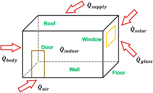
FIGURE 1. Schematic diagram of building thermal processes through envelopes.

Based on aforementioned assumptions, the heat balance equation for indoor air can be expressed by Eq. 1.

${\rho }_{air}{C}_{air}{V}_{room}\frac{d{T}_{air,inside}\left(\tau \right)}{d\tau }={\dot{Q}}_{body}+{\dot{Q}}_{glass}+{\dot{Q}}_{solar}+{\dot{Q}}_{air}+{\dot{Q}}_{supply}+{\dot{Q}}_{indoor}(1)$

Where: ${\rho }_{air}$ is the air density, kg/m³; $C_{air}$ is the specific heat capacity of air, J/(kg·K); $V_{room}$ is the room volume, m³; $T_{air,inside}\left(\tau \right)$ is the indoor air temperature (IAT) at time $\tau$, °C; ${\dot{Q}}_{body}$ is the heat exchange through non-transparent envelope, W; ${\dot{Q}}_{glass}$ is the heat exchange through transparent building envelope, W; ${\dot{Q}}_{solar}$ is the solar radiation transmitted by transparent building envelope, W; ${\dot{Q}}_{air}$ is the heat exchange caused by air leakage, W; ${\dot{Q}}_{indoor}$ is the heat emitted by personnel, lighting, equipment, etc., W; without regard to inner heat source, ${\dot{Q}}_{indoor}$ was 0; ${\dot{Q}}_{supply}$ the heat provided by air conditioning and heating equipment, W. The calculation formula of ${\dot{Q}}_{body}$, ${\dot{Q}}_{glass}$, ${\dot{Q}}_{air}$ can be expressed by (2) (3) (4). Where: $h_i$ is the convective heat transfer coefficient between the inner surface $i$ of the non-transparent envelope and the indoor air, W/(m²·K); $A_i$ is the heat transfer area of the inner surface $i$ of the non-transparent envelope, m²; $T_{wall,i}\left(\tau \right)$ is the wall temperature of the inner surface $i$ of the non-transparent envelope, °C. $N_{bodies}$ is the number of the non-transparent envelopes.

${\dot{Q}}_{body}={\displaystyle {\sum }_{i=1}^{N_{bodies}}}{h}_{inside,i}{A}_i\left[T_{surface,inside,i}\left(\tau \right)-T_{air,inside}\left(\tau \right)\right](2)$

Where: $K_{glass,j}$ is the comprehensive heat transfer coefficient of the transparent building envelope $j$, W/(m²·K); $A_j$ is the heat transfer area of the transparent building envelope $j$, m²; $T_{air,outside}\left(\tau \right)$ is outdoor air temperature at time $\tau$, °C; $N_{glasses}$ is the number of the transparent envelopes.

${\dot{Q}}_{glass}={\displaystyle {\sum }_{j=1}^{N_{glasses}}}{K}_{glass,j}{A}_j\left[T_{air,outside}\left(\tau \right)-T_{air,inside}\left(\tau \right)\right](3)$

Where: $m_{\mathit{inf}}$ is the ventilation volume between indoor and outdoor, kg/s. The calculation formula is given by Eq. 5 (Zhang, 2006).

${\dot{Q}}_{air}=m_{\mathit{inf}}{C}_{air}\left[T_{air,outside}\left(\tau \right)-T_{air,inside}\left(\tau \right)\right](4)$

$m_{\mathit{inf}}=\frac{n_k{V}_{room}{\rho }_{air}}{3600}(5)$

2.2 Building envelope heat transfer

The non-transparent envelope essentially incorporated walls, floors, doors. Due to thermal inertia, the heat transfer process could be supposed to be one-dimensional unsteady heat transfer process (Figure 2). Consequently, the heat transfer model was described by the heat conduction Eq 6 which also illustrated the temperature distribution inside the solid.

$\frac{\partial T_{wall}\left(x,t\right)}{\partial \tau }=\frac{\lambda }{{\rho }_{wall}{C}_{wall}}\frac{\partial T_{wall}^2\left(x,t\right)}{\partial x^2}(6)$

Where: $T_{wall}$ is wall temperature, °C; $\tau$ is heat transfer time, s; $\rho$ is wall density, kg/m³; $c_p$ is specific heat capacity, J/(kg·K); $\lambda$ is thermal conductivity, W/(m·K); $x$ is the distance in the direction of wall thickness, m. The thermal balance analysis of the non-transparent envelope surfaces plays an important role on building theoretical models. Assuming that the $c_p$ of the thin layer on the surface is nearly 0, the heat balance diagram of the outer surface $i$ is shown in Figure 3, and the heat balance equation is shown in Eq. 7. When without solar radiation, ${\dot{q}}_{solar,i}$ and ${\dot{q}}_{clear,i}$ were both 0.

${\dot{q}}_{solar,i}+{\dot{q}}_{clear,i}+{\dot{q}}_{convection,outside,i}+{\dot{q}}_{wall,outside,i}=0(7)$

Where: ${\dot{q}}_{solar,i}$ is absorbed solar radiation, W/m²; ${\dot{q}}_{clear,i}$ is the total net radiation heat transfer between the surface $i$ and the ground, sky, and air, W/m²; ${\dot{q}}_{convection,outside,i}$ is the convective heat transfer between the surface $i$ and air, W/m²; ${\dot{q}}_{wall,outside,i}$ is the conductive heat transfer, W/m². ${\dot{q}}_{convection,outside,i}$ is addressed by

${\dot{q}}_{convection,outside,i}=h_{outside,i}\left[T_{air,outside}\left(\tau \right)-T_{surface,outside,i}\left(\tau \right)\right](8)$

Where: $h_{outside,i}$ is the convective heat transfer coefficient, W/(m²·K). ${\dot{q}}_{wall,outside,i}$ plays an important role on unsteady heat transfer calculations, it is expressed as

${\dot{q}}_{wall,outside,i}=K_{node,i,1}\left[T_{node,i,1}\left(\tau \right)-T_{surface,outside,i}\left(\tau \right)\right](9)$

Where: $T_{node,i,1}\left(\tau \right)$ is the temperature of the first node, K; $K_{node,i,1}$ is the heat-transfer coefficient of the first node, it is expressed as

$K_{node,i,1}=\frac{{\lambda }_{node,i,1}}{{\delta }_{node,i,1}}(10)$

Where: ${\lambda }_{node,i,1}$ is the thermal conductivity, W/(m·K); ${\delta }_{node,i,1}$ is the thickness, m. Theoretically, the radiation heat transfer between the internal surfaces is complicated. On the one hand, radiation heat transfer occurs between any surface, including transmission and reflection of projection; on the other hand, the apparent thermal radiation is closely related to the surface properties. However, the radiation heat transfer between internal surfaces is usually negligible compared to the received solar radiation in engineering calculations. Hence, the diagram of the thermal balance of the interior surface is shown in (11), and the heat balance equation is established as:

${\dot{q}}_{rad,1,i}+{\dot{q}}_{rad,2,i}+{\dot{q}}_{convection,inside,i}+{\dot{q}}_{wall,inside,i}=0(11)$

Where: ${\dot{q}}_{rad,1,i}$ is the radiation heat transfer between internal surfaces, W/m²; According to assumption (7), it is negligible; ${\dot{q}}_{rad,2,i}$ is the solar heat gain through window, W/m²; ${\dot{q}}_{convection,inside,i}$ is the convective heat transfer, W/m²; ${\dot{q}}_{wall,inside,i}$ is the heat transfer of the first node adjacent to the internal surface, W/m². When without solar radiation, ${\dot{q}}_{rad,1,i}$ and ${\dot{q}}_{rad,2,i}$ are both 0. Based on assumption (3), there are:

${\dot{q}}_{rad,2,i}=0.7\cdot \frac{{\displaystyle {\sum }_{j=1}^{N_{glasses}}}{{SHG{C}_j\cdot I}_{total,j}\left(\tau \right)\cdot A}_j}{A_{ground}}(12)$

${\dot{q}}_{rad,2,i}=0.3\cdot \frac{{\displaystyle {\sum }_{j=1}^{N_{glasses}}}{{SHG{C}_j\cdot I}_{total,j}\left(\tau \right)\cdot A}_j}{{\displaystyle {\sum }_{i=1}^{N_{bodies}}}{A}_i}(13)$

${\dot{q}}_{convection,inside,i}=h_{inside,i}\left[T_{surface,inside,i}\left(\tau \right)-T_{air,inside}\left(\tau \right)\right](14)$

${\dot{q}}_{wall,outside,i}=K_{node,i,n}\left[T_{node,i,n}\left(\tau \right)-T_{surface,inside,i}\left(\tau \right)\right](15)$

Where: $SHGC$ is the solar heat gain coefficient of window $j$; $A_{ground}$ is the ground area, m²; $A_i$ is the area of surface $i$, m²; $h_{inside,i}$ is the convective heat transfer coefficient between internal surface and air, W/(m²·K); $T_{surface,inside,i}\left(\tau \right)$ is the temperature at time $\tau$,°C; $T_{node,i,n}\left(\tau \right)$ is the temperature of node $n$ in surface $i$, °C; $K_{node,i,n}$ is the heat-transfer coefficient of the first node, W/(m²·K).

FIGURE 2

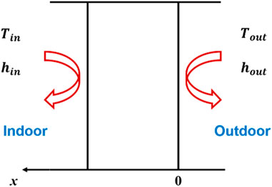
FIGURE 2. Heat conduction and convections for building walls.

FIGURE 3

FIGURE 3. Boundary condition for external heat balance.

2.3 Governing equations

Eq. 16 is a partial differential equation. Wide-used methods for solving this equation mainly depends on finite difference approaches (Ding et al., 2004; Long, 2005; He and Ding, 2011; Pan, 2013). The core of theoretical calculation is to connect the ambient and indoor temperatures via scientific methods. Accordingly, the energy conservation of indoor air nodes cannot be ignored. In addition, the operability of the model calculation should be considered. Therefore, we applied the numerical method to solve the problem. The node diagram is shown in Figure 4.

FIGURE 4

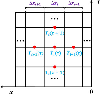
FIGURE 4. Diagram of node division.

For the three consecutive nodes at time $\tau$ in Figure 4; Eq. 6 can be transformed into Eq. 16 in a differential form.

$\frac{T_i\left(\tau \right)-T_i\left(\tau -1\right)}{⊿\tau }=\frac{1}{c_i{\rho }_i⊿x_i}\left[\frac{T_{i+1}\left(\tau \right)-T_i\left(\tau \right)}{\frac{1}{2}\left(\frac{⊿x_i}{{\lambda }_i}+\frac{⊿x_{i+1}}{{\lambda }_{i+1}}\right)}-\frac{T_i\left(\tau \right)-T_{i-1}\left(\tau \right)}{\frac{1}{2}\left(\frac{⊿x_{i-1}}{{\lambda }_{i-1}}+\frac{⊿x_i}{{\lambda }_i}\right)}\right](16)$

Where: $c_i$ is the specific heat of node $i$, J/(kg·K); ${\rho }_i$ is the density of node $i$, kg/m³; $⊿x_{i-1}$, $⊿x_i$, $⊿x_{i+1}$ are the lengths of nodes $i-1$, $i$, $i-1$ respectively, m; ${\lambda }_{i-1}$, ${\lambda }_i$, ${\lambda }_{i+1}$ are the thermal conductivity of nodes $i-1$, $i$, $i-1$ respectively, W/(m·K). Eq. 16 can be transformed into Eqs 17, 18, which is the thermal conductivity equation for each node. To solve it, the boundary conditions of the third kind are erected to form a system of equations with an unknown number equal to the number of equations. The thermal equilibrium method is employed to establish equations for the internal and external surfaces.

$a_{i,i-1}{T}_{i-1}\left(\tau \right)+a_{i,i}{T}_i\left(\tau \right)+a_{i,i+1}{T}_{i+1}\left(\tau \right)=-T_i\left(\tau -1\right)(17)$

$\text{Wherein}:\left\{\begin{array}{c}{a}_{i,i-1}=\frac{2⊿\tau }{c_i{\rho }_i⊿x_i\left(\frac{⊿x_{i-1}}{{\lambda }_{i-1}}+\frac{⊿x_i}{{\lambda }_i}\right)}\\ a_{i,i}=-\left\{\frac{2⊿\tau }{c_i{\rho }_i⊿x_i}\left[\frac{1}{\left(\frac{⊿x_{i-1}}{{\lambda }_{i-1}}+\frac{⊿x_i}{{\lambda }_i}\right)}+\frac{1}{\left(\frac{⊿x_i}{{\lambda }_i}+\frac{⊿x_{i+1}}{{\lambda }_{i+1}}\right)}\right]+1\right\}\\ a_{i,i+1}=\frac{2⊿\tau }{c_i{\rho }_i⊿x_i\left(\frac{⊿x_i}{{\lambda }_i}+\frac{⊿x_{i+1}}{{\lambda }_{i+1}}\right)}\end{array}\right.(18)$

$\begin{array}{ll}\hfill {\rho }_{air}{C}_{air}{V}_{room}\frac{d{T}_{air,inside}\left(\tau \right)}{d\tau }& ={\displaystyle {\sum }_{i=1}^{N_{bodies}}}{h}_i{A}_i\left[T_{surface,inside,i}\left(\tau \right)-T_{air,inside}\left(\tau \right)\right]+{\displaystyle {\sum }_{j=1}^{N_{glasses}}}{h}_j{A}_j\left[T_{air,outside}\left(\tau \right)-T_{air,inside}\left(\tau \right)\right]\hfill \\ \hfill & +\frac{n_k{V}_{room}{\rho }_{air}}{3600}{C}_{air}\left[T_{air,outside}\left(\tau \right)-T_{air,inside}\left(\tau \right)\right]+Q_{supply}\left(\tau \right)\hfill \end{array}(19)$

According to the first-order forward difference format, Eq. 19 can be converted to:

$\begin{array}{ll}\hfill {\rho }_{air}{C}_{air}{V}_{room}\frac{T_{air,inside}\left(\tau \right)-T_{air,inside}\left(\tau -1\right)}{⊿\tau }& ={\displaystyle {\sum }_{i=1}^{N_{bodies}}}{h}_{inside,i}{A}_i{T}_{surface,inside,i}\left(\tau \right)-{\displaystyle {\sum }_{i=1}^{N_{bodies}}}{h}_{inside,i}{A}_i{T}_{air,inside}\left(\tau \right)+{\displaystyle {\sum }_{j=1}^{N_{glasses}}}{K}_{glass,j}{A}_j{T}_{air,outside}\left(\tau \right)\hfill \\ \hfill & -{\displaystyle {\sum }_{j=1}^{N_{glasses}}}{K}_{glass,j}{A}_j{T}_{air,inside}\left(\tau \right)+\frac{n_k{V}_{room}{\rho }_{air}{C}_{air}}{3600}{T}_{air,outside}\left(\tau \right)-\frac{n_k{V}_{room}{\rho }_{air}{C}_{air}}{3600}{T}_{air,inside}\left(\tau \right)+Q_{supply}\left(\tau \right)\hfill \end{array}(20)$

The expression for IAT at time $\tau$ is expressed as:

$T_{air,inside}\left(\tau \right)=\frac{\begin{array}{c}\frac{{\rho }_{air}{C}_{air}{V}_{room}{T}_{air,inside}\left(\tau -1\right)}{⊿\tau }+{\displaystyle {\sum }_{i=1}^{N_{bodies}}}{h}_{inside,i}{A}_i{T}_{surface,inside,i}\left(\tau \right)+\\ \frac{n_k{V}_{room}{\rho }_{air}{C}_{air}{T}_{air,outside}\left(\tau \right)}{3600}+{\displaystyle {\sum }_{j=1}^{N_{glasses}}}{K}_{glass,j}{A}_j{T}_{air,outside}\left(\tau \right)+Q_{supply}\left(\tau \right)\end{array}}{\frac{{\rho }_{air}{C}_{air}{V}_{room}}{⊿\tau }+{\displaystyle {\sum }_{i=1}^{N_{bodies}}}{h}_{inside,i}{A}_i+{\displaystyle {\sum }_{j=1}^{N_{glasses}}}{K}_{glass,j}{A}_j+\frac{n_k{V}_{room}{\rho }_{air}{C}_{air}}{3600}}(21)$

When without solar radiation, the expression for IAT at time τ is expressed as:

$T_{air,inside}\left(\tau \right)=\frac{\begin{array}{c}\frac{{\rho }_{air}{C}_{air}{V}_{room}{T}_{air,inside}\left(\tau -1\right)}{⊿\tau }+{\displaystyle {\sum }_{i=1}^{N_{bodies}}}{h}_{inside,i}{A}_i{T}_{surface,inside,i}\left(\tau \right)+\\ \frac{n_k{V}_{room}{\rho }_{air}{C}_{air}{T}_{air,outside}\left(\tau \right)}{3600}+Q_{supply}\left(\tau \right)\end{array}}{\frac{{\rho }_{air}{C}_{air}{V}_{room}}{⊿\tau }+{\displaystyle {\sum }_{i=1}^{N_{bodies}}}{h}_{inside,i}{A}_i++\frac{n_k{V}_{room}{\rho }_{air}{C}_{air}}{3600}}(22)$

When with solar radiation, the heat balance equation of internal wall is addressed by Eq. 23. For the convenience of expression, the directly accepted solar radiation (including direct and scattered radiation) is represented by $I_{total}\left(\tau \right)$. Meanwhile, we adopted $T_{surface,inside}\left(\tau -1\right)$ to approximately replace $T_{surface,inside}\left(\tau \right)$.

$\begin{array}{ll}\hfill \left(h_{outside}+K_{node,1}\right)T_{surface,outside}\left(\tau \right)-K_{node,1}{T}_{node,1}\left(\tau \right)& =h_{outside}{T}_{air,outside}\left(\tau \right)+{\alpha }_{solar}{I}_{total}\left(\tau \right)\hfill \\ \hfill & +{\epsilon }_i\sigma F_{ground,i}\left[T_{ground,i}^4\left(\tau \right)-T_{surface,outside}^4\left(\tau -1\right)\right]\hfill \\ \hfill & +{\epsilon }_i\sigma F_{sky,i}\left[T_{sky}^4\left(\tau \right)-T_{surface,outside}^4\left(\tau -1\right)\right]\hfill \end{array}(23)$

When without solar radiation, the heat balance equation of internal wall is expressed as:

$\left(h_{outside}+K_{node,1}\right)T_{surface,outside}\left(\tau \right)-K_{node,1}{T}_{node,1}\left(\tau \right)=h_{outside}{T}_{air,outside}\left(\tau \right)(24)$

After dispersing, the heat balance equation of ground and other envelopes are expressed as:

${\displaystyle {\sum }_{j=1}^{N_{glasses}}}{I_{total}\left(\tau \right)A}_j+h_{inside}{T}_{air,inside}\left(\tau \right)(25)$

$\left(h_{inside}+K_{node,n}\right)T_{surface,inside}\left(\tau \right)-K_{node,n}{T}_{node,n}\left(\tau \right)=0.3\cdot SHGC\cdot \frac{{\displaystyle {\sum }_{j=1}^{N_{glasses}}}{I_{total}\left(\tau \right)A}_j}{{\displaystyle {\sum }_{i=1}^{N_{bodies}}}{A}_i}+h_{inside}{T}_{air,inside}\left(\tau \right)(26)$

$\left(h_{inside}+K_{node,n}\right)T_{surface,inside}\left(\tau \right)-K_{node,n}{T}_{node,n}\left(\tau \right)=h_{inside}{T}_{air,inside}\left(\tau \right)(27)$

2.4 Dynamic numerical solution

The building room thermal process can be decomposed into several sets of equations. The equations without and with solar radiation were shown in Eqs 28, 29, respectively.

$\left[\begin{array}{ccccc}\left(h_{outside}-K_{node,1}\right)& -K_{node,1}& 0& \cdots & 0\\ a_{1,0}& a_{1,1}& a_{1,2}& \cdots & 0\\ \cdots & \cdots & \cdots & \cdots & \cdots \\ 0& \cdots & a_{3,2}& a_{3,3}& a_{3,4}\\ 0& 0& \cdots & -K_{node,n}& \left(h_{inside}+K_{node,n}\right)\end{array}\right]\cdot \left[\begin{array}{c}{T}_{surface,outside}\left(\tau +1\right)\\ T_1\left(\tau +1\right)\\ \cdots \\ T_n\left(\tau +1\right)\\ T_{surface,inside}\left(\tau +1\right)\end{array}\right]=\left[\begin{array}{c}{h}_{outside}{T}_{air,outside}\left(\tau +1\right)\\ -T_1\left(\tau \right)\\ \cdots \\ -T_n\left(\tau \right)\\ h_{inside}{T}_{air,inside}\left(\tau +1\right)\end{array}\right](28)$

$\left[\begin{array}{ccccc}\left(h_{outside}-K_{node,1}\right)& -K_{node,1}& 0& \cdots & 0\\ a_{1,0}& a_{1,1}& a_{1,2}& \cdots & 0\\ \cdots & \cdots & \cdots & \cdots & \cdots \\ 0& \cdots & a_{3,2}& a_{3,3}& a_{3,4}\\ 0& 0& \cdots & -K_{node,n}& \left(h_{inside}+K_{node,n}\right)\end{array}\right]\cdot \left[\begin{array}{c}{T}_{surface,outside}\left(\tau +1\right)\\ T_1\left(\tau +1\right)\\ \cdots \\ T_n\left(\tau +1\right)\\ T_{surface,inside}\left(\tau +1\right)\end{array}\right]=\left[\begin{array}{c}{h}_{outside}{T}_{air,outside}\left(\tau +1\right)+{\alpha }_{solar}{I}_{total}\left(\tau \right)+{\dot{q}}_{clear,i}\\ -T_1\left(\tau \right)\\ \cdots \\ -T_n\left(\tau \right)\\ h_{inside}{T}_{air,inside}\left(\tau +1\right)+{\dot{q}}_{rad,2,i}\end{array}\right](29)$

The forward differential governing equations have an implicit structure. The solving is stable, and the time step does not influence the accuracy of the results. The numerical solution process in Matlab is demonstrated in Figure 5.

FIGURE 5

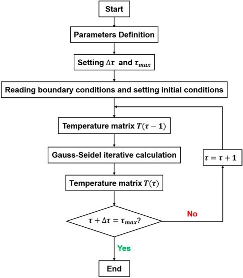
FIGURE 5. Flow chat of dynamic solution process.

When the indoor air temperature is known, the heating load is expressed as:

$Q_{heating}=\left\{\begin{array}{c}{C}_{air}{\rho }_{air}{V}_{room}\left[T_{set}-T_{air,inside}\left(\tau \right)\right]T_{set}>T_{air,inside}\left(\tau \right)\\ 0T_{set}\le T_{air,inside}\left(\tau \right)\end{array}\right.(30)$

3 Experiment

To overcome challenges related to controlling changing parameters in actual buildings and the intricate coupling effects of various factors on IAT, the modelling case boxes are set up for onsite test (Chen et al., 2021; Qian et al., 2022; Guo et al., 2023). This approach aimed to investigate the impact of different factors on indoor air temperature changes in model buildings under similar environmental conditions, while accounting for solar radiation. Model building N consisted entirely of particle panels (non-transparent envelopes), impervious to solar radiation. It was divided into two groups: N1. In contrast, model building S comprised fully glass (transparent enclosure structure) facing the south, allowing solar radiation penetration. Corresponding to model building N, model building S also had two groups, named S1, S2. Summarily, Table 1 compiles the key characteristics of the model buildings. The experiment was carried out on a hotel proof in Songpan District (103°24′E, 32°40′N), Sichuan Province, China. Unobstructed sunlight was available as there were no mountains or structures blocking it. The experiment took place from December 4th to 10th, 2022, and the weather remained clear throughout the testing period.

TABLE 1

TABLE 1. Designed working conditions.

3.1 Model building

For the convenience of experimentation, we modeled the building based on similarity model theory (Zhou and Lv, 2012), shrinking the actual building model into a rectangular box measuring 800 mm in length, 600 mm in width, and 500 mm in height according to correlation factors. This approach effectively reduces both the building and the variables under study to the same degree, ensuring the persuasiveness of the experiment. The expandable polystyrene (EPS) was used for thermal insulation. Detailed experiment design parameters are shown in Figure 6. The thermal conductivity particle boards, EPS, and glass were measured using a thermal conductivity tester. The results show that the thermal conductivity of EPS is 0.0345 W/(m·K), and that of glass is 0.19 W/(m·K). The thermal parameters of the model building materials are summarized in Table 2.

FIGURE 6

FIGURE 6. Description of the model building: (A) dimensions; (B) physical drawings.

TABLE 2

TABLE 2. Basic parameters of the model building.

3.2 Instruments and sensors

The instruments utilized in this experiment are shown in Figure 7; Table 3. However, due to the high proportion of direct radiation in the Songpan district, cloud and fog occlusion could easily lead to large temperature fluctuations, so we did not repeat the experiments to analyze the uncertainty.

FIGURE 7

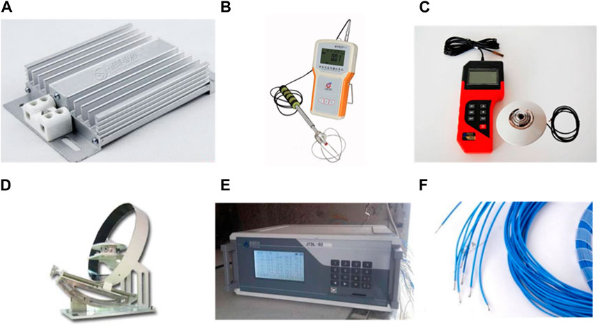
FIGURE 7. Physical picture of experimental instruments: (A) 100W electric heater; (B) universal anemometer; (C) total solar radiation recorder; (D) solar scattering radiation recorder; (E) multi-channel data acquisition system; (F) Thermocouple.

TABLE 3

TABLE 3. Details of the sensors.

3.3 On-site testing

Experimental data were captured using a multi-channel acquisition system, detailed in Figure 8. The corresponding regional solar radiation intensities are shown in Figure 9. To elaborate on the experimental setup, thermocouples were strategically positioned on both the internal and external surfaces. Notably, each model building was equipped with a central thermocouple to monitor indoor air temperature. In order to minimize errors stemming from direct solar radiation, each thermocouple was meticulously affixed with tin foil paper. All thermocouples were subjected to calibration within a water bath prior to testing, ensuring consistency in initial temperature readings. Importantly, the models were positioned in a manner that did not obstruct each other. The experimental setup further incorporated a universal anemometer and a solar radiation recorder, positioned approximately 1 m from the model building. These devices facilitated the recording of wind velocity and solar radiation.

FIGURE 8

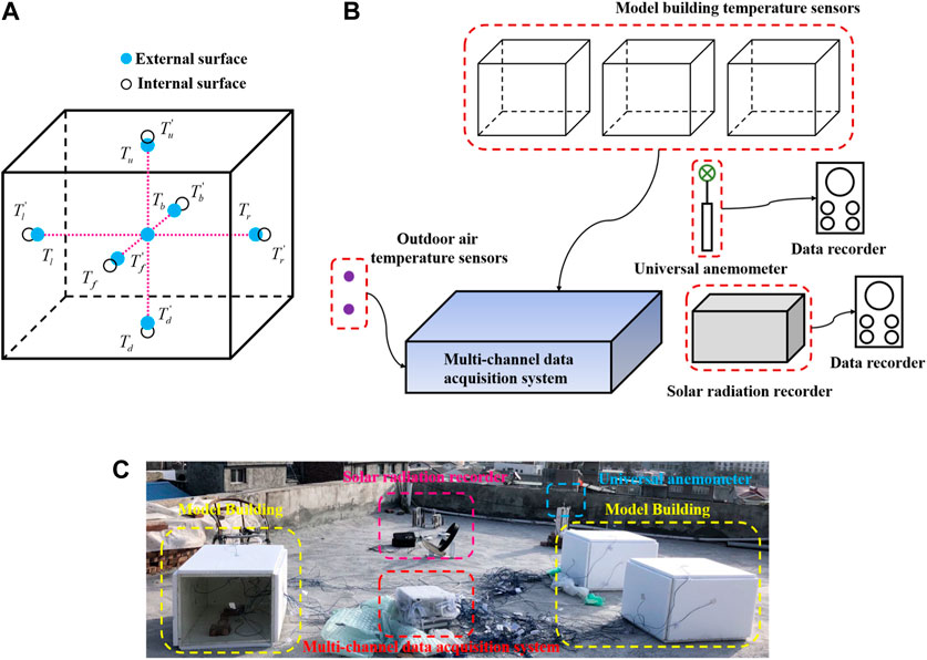
FIGURE 8. Details of the experimental system: (A) measuring point in model buildings; (B) schematic diagram of data collection system; (C) site layout.

FIGURE 9

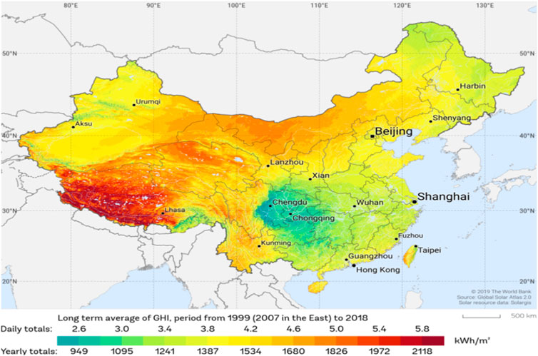
FIGURE 9. Distribution map of solar radiation intensity in China.

Throughout the testing process, the recorder logged values on a minute-by-minute basis, while temperature data were averaged every 10 minutes to mitigate errors arising from unforeseen circumstances.

3.4 Uncertainty analysis

The uncertainty analysis aims to assess the reliability and accuracy of experimental results, considering both accidental errors (Type-A uncertainty) and instrument errors (Type-B uncertainty). Calculating the Type-A uncertainty by repeating the experiment posed challenges and rendered it meaningless due to the weather’s unpredictability. Therefore, we opted to Type-B uncertainty. In this particular experiment, the Type-B uncertainty primarily stemmed from inaccuracies in measuring temperature ($T$), wind speed ($u$) and the solar radiation ($q_{solar}$). As a result, we determine the uncertainty of the experimental outcomes using Eqs 31, 32 (Ma et al., 2022). After calculation, the overall uncertainty of the experiment results was 2.4%.

$f=f\left(T,u,q_{solar}\right)(31)$

$\Delta f=\sqrt{{\left(\frac{\delta T}{{\left|T\right|}_{\mathit{max}}}\right)}^2+{\left(\frac{\delta u}{{\left|u\right|}_{\mathit{max}}}\right)}^2+{\left(\frac{\delta q_{solar}}{{\left|q_{solar}\right|}_{\mathit{max}}}\right)}^2}(32)$

4 Results and discussion

By comprehensively considering wall thermal inertia, as well as heat transfer with and without with and without solar radiation, separate validations are considered for three aspects to thoroughly demonstrate the model’s accuracy and applicability.

4.1 Wall thermal responses

Figure 10 presents a comparison between the experimental and simulated surface temperatures. The trend of simulated internal and external wall temperatures aligns with the experimental values. The wall material, particle board, possesses significantly lower thermal inertia than conventional building materials, with a mere thickness of 0.018 m. Therefore, the simulation indicates a close proximity between internal and external wall temperatures. The differences between them-maximum, minimum, and average-are only 0.1°C, −0.2°C, and 0.02°C, respectively. Similarly, the disparities between simulated and experimental external wall temperatures yield values of 2.4°C, −4.2°C, and 0.6°C, respectively. The average error, based on experimental external wall temperature, stands at 4.9%.

FIGURE 10

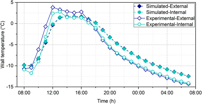
FIGURE 10. Comparison between the wall surface temperatures.

Furthermore, it’s important to consider two factors. Firstly, given the substantial range of temperature fluctuations, errors in calculation may lead to both positive and negative offsets. Secondly, as temperatures approach 0°C, even a minor difference can result in a significant error. The absolute ratio of average error to the maximum experimental value is 4.6%. Additionally, the maximum, minimum, and average difference between the simulated and experimental values of the internal wall temperature was 2.5°C, −4.2°C, and 0.7°C, respectively.

4.2 Comparison between with/without solar radiation consideration

The heat transfer model, excluding solar radiation, was established based on a traditional model that removed the effects of absorbed, transmitted, and reflected solar radiation. Additionally, it neglected radiative heat transfer between the building surface and the environment. Given its inherent hypothetical nature, completely isolating solar radiation and radiative heat exchange during field measurements proved challenging, Consequently, validating the mathematical model posed significant difficulty. Nonetheless, comparative experimental conditions were devised to specifically isolate transmitted solar radiation during the experimental tests. To approximate the accuracy of the mathematical model, measured data from the model building N were employed. Hence, for validation purposes, four sets of results from model building N1 and model building N3 were chosen.

Figure 11 shows the comparison results of N1 under natural condition. The simulated values closely aligned with the experimental values, showcasing a minimal average temperature difference of 0.1°C. Additionally, the absolute ratio of the average error to the highest experimental value stood at a mere 0.7%. Notably, there exists a nuanced distinction between simulation and experiment results. During daylight hours, the simulation values were slightly lower than the experimental values, a phenomenon attributed to the long-wave radiation exchanged between the building’s external surfaces and the surrounding environment. Conversely, during the night, a marginal rise in simulation values relative to experimental values was observed. This is possibly due to the absence of glass in N1. Conversely, during the day, despite N1 not transmitting solar radiation, the external walls would still absorb solar radiation, leading to experimental values surpassing the simulated values.

FIGURE 11

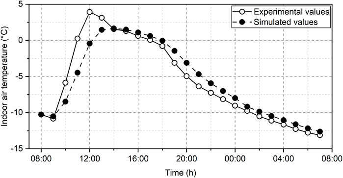
FIGURE 11. IATs of N1 under natural conditions.

Figure 12 illustrates a comparison of results for N2 under natural conditions. Analogous to previous cases, during daylight hours, simulation values were lower than their experimental counterparts, while during nighttime, simulation values surpassed the experimental data. The statistical differences between them were as follows: an average temperature difference of −0.7°C, a maximum of 0.5°C, and a minimum of −2.5°C. Additionally, the absolute ratio of the average error to the highest experimental value remained minimal, at 6.4%. Notably, the overall trends of simulation and experimental values aligned consistently.

FIGURE 12

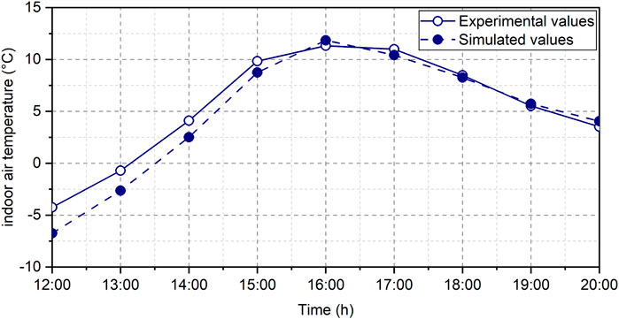
FIGURE 12. IATs of N2 under natural conditions.

Figure 13 displays a comparison of results for model building N1 under heating conditions. Unlike the situation with natural conditions, simulation values did not exhibit lower values than the experimental values during the daytime. This shift can be attributed to heating becoming the predominant influencing factor. Moreover, the influence of solar radiation absorbed by the building’s external wall surfaces, as represented in the theoretical model, becomes less pronounced. The statistical disparities between simulation and experimental data were as follows: an average temperature difference of 1.6°C, a maximum of 5.4°C, and a minimum of −1.1°C. Furthermore, the absolute ratio of the average error to the highest experimental value was calculated at 7.7%.

FIGURE 13

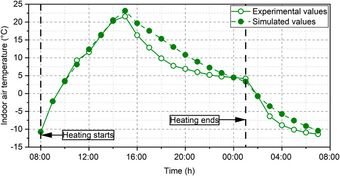
FIGURE 13. IATs of N1 under heating conditions.

Figure 14 shows a comparison of results for model building N2 under heating conditions. During daytime heating, the simulation values exhibited remarkable alignment with the experimental values. As observed in model building N1, simulation values remained elevated compared to experimental values following the cessation of heating at night. This can be attributed to the theoretical model’s omission of the influence stemming from long-wave radiation exchanged between the building’s external surfaces and the outdoor environment. The overall disparity between the two values was captured through statistical measures. The average temperature difference stood at 1.9°C, with a maximum difference of 5.3°C and a minimum difference of −0.8°C. Notably, the absolute value of the highest proportion of average error registered a mere 0.5%.

FIGURE 14

FIGURE 14. IATs of N2 under heating conditions.

In contrast to heat transfer models that exclude solar radiation, those incorporating solar radiation take into account its impact, aligning them with traditional building heat transfer models. Thus, the validation process was executed using the measured data from model building S1. Figure 15 visually portrays the IATs for model building S1 under natural conditions. The observed disparity between simulated and experimental data is more pronounced during daylight hours when solar radiation is considered, and less marked during nighttime when solar radiation is absent. This phenomenon can be attributed to two primary factors. Firstly, the solar radiation data employed in the theoretical model is based on measurements; however, inherent instrumentation limitations might cause measured values to be lower than actual values. Moreover, the measured data was sampled at 1-min intervals. To facilitate calculations, an hourly average was employed to mitigate peak solar radiation. Secondly, despite precautions taken in the experimental setup to minimize direct sunlight exposure, the thermocouple measuring indoor air temperature could not entirely avoid absorbing sunlight, leading to localized temperature elevation. In contrast, the theoretical model operates in an ideal environment, calculating indoor air temperature with minimal external influences. Quantitatively, the average temperature difference between simulated and experimental values is 1.1°C, with a maximum temperature difference of 6°C. The absolute ratio of the average error to the highest experimental value remains exceptionally low at 0.5%.

FIGURE 15

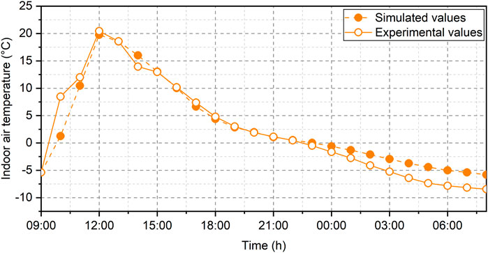
FIGURE 15. IATs of S1 under natural conditions.

Figure 16 visually represents the IATs for model building S2 under heating conditions. Notably, at the initial phase of heating, simulated values exceeded experimental values. This discrepancy can be attributed to potential differences between actual heating power and the tested value, potentially leading to pronounced calculation results. Post 13:00, simulation values exhibited substantial fluctuations, mainly due to the unpredictable impact of intermittent cloud cover. Quantitatively, the average temperature difference between simulated and experimental values is 1°C, with a maximum temperature difference of 2.7°C. Importantly, the absolute ratio of the average error to the highest experimental value remains remarkably low at 2.1%.

FIGURE 16

FIGURE 16. IATs of S2 under heating conditions.

4.3 Evaluation and validation

The validation of model results was conducted through visual analysis in the preceding article. To comprehensively expound the alignment between experimental and simulated results, we adopted the root mean square deviation ($RMSD$) and the coefficient of variation ($CV$) as evaluation metrics (Vogt et al., 2018; Li et al., 2020). The calculation formulas are expressed as:

$RMSD=\sqrt{\frac{{\displaystyle {\sum }_{i=1}^N}{\left(t_E-t_s\right)}^2}{N}}(33)$

$CV=\frac{RMSD}{\overline{\left|t_E\right|}}\times 100\%(34)$

Where: $t_E$ is the experimental value, °C; $t_s$ is the simulated value, °C.

Table 4 presents the comparison results for $RMSD$ and $CV$. It is noteworthy that all $CV$ values fall below 30%, indicating the model’s substantial reliability.

TABLE 4

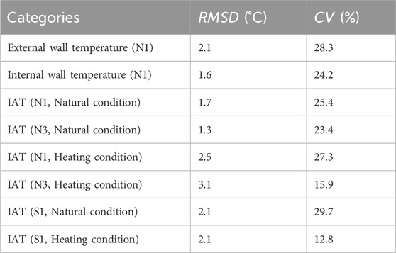
TABLE 4. The results of RMSD and CV.

5 Conclusion

In this paper, a modified and improved dynamic thermal design model is put forward for built environment and energy consumption estimation for passive buildings for plateau buildings. Moreover, the simplified experiment is set up to monitor dynamic thermal responses for modelling building. The onsite experiment indicates that window-to-wall ratios, architectural orientation, thermal insulation coefficients, have substantial impacts for solar heat gains in plateau buildings. In addition, the data validation between model simulation and experiment involves various influence impacts, especially on wall heat transfer models with and without solar radiation considerations. The preliminary validation results demonstrate that the proposed thermal model accuracy is quite desirable in engineering applications, with the coefficient of variation (CV) ranging within 30%, denoting the model robust reliability. The study renders building design guidance for energy conservation in high altitude plateau areas.

Data availability statement

The raw data supporting the conclusion of this article will be made available by the authors, without undue reservation.

Author contributions

YZ: Conceptualization, Writing–original draft. WH: Data curation, Formal Analysis, Validation, Writing–review and editing. YQ: Project administration, Supervision, Writing–review and editing.

Funding

The author(s) declare financial support was received for the research, authorship, and/or publication of this article. This work is supported by National Natural Science Foundation of China (No. 52308038) and Higher Education Reform Research Project of National Ethnic and Religious Affairs Commission of China (No. 23022).

Acknowledgments

The authors would like to express sincere gratitude to research fellows from School of Architecture and Environment, Sichuan University, China.

Conflict of interest

The authors declare that the research was conducted in the absence of any commercial or financial relationships that could be construed as a potential conflict of interest.

Publisher’s note

All claims expressed in this article are solely those of the authors and do not necessarily represent those of their affiliated organizations, or those of the publisher, the editors and the reviewers. Any product that may be evaluated in this article, or claim that may be made by its manufacturer, is not guaranteed or endorsed by the publisher.

References

Al-Janabi, A., Kavgic, M., Mohammadzadeh, A., and Azzouz, A. (2019). Comparison of EnergyPlus and IES to model a complex university building using three scenarios: free-floating, ideal air load system, and detailed. J. Build. Eng. 22, 262–280. doi:10.1016/j.jobe.2018.12.022

CrossRef Full Text | Google Scholar

Alwetaishi, M., Balabel, A., Abdelhafiz, A., Issa, U., Sharaky, I., Shamseldin, A., et al. (2020). User thermal comfort in historic buildings: evaluation of the potential of thermal mass, orientation, evaporative cooling and ventilation. Orientat. Evaporative Cool. Vent. 12, 9672. doi:10.3390/su12229672

CrossRef Full Text | Google Scholar

Cao, W., Yu, J., Chao, M., Wang, J., Yang, S., Zhou, M., et al. (2023). Short-term energy consumption prediction method for educational buildings based on model integration. Energy 283, 128580. doi:10.1016/j.energy.2023.128580

CrossRef Full Text | Google Scholar

Chen, J., Lu, L., Gong, Q., Wang, B., Jin, S., and Wang, M. (2021). Development of a new spectral selectivity-based passive radiative roof cooling model and its application in hot and humid region. J. Clean. Prod. 307, 127170. doi:10.1016/j.jclepro.2021.127170

CrossRef Full Text | Google Scholar

Chen, Y., Quan, M., Wang, D., Du, H., Hu, L., Zhao, Y., et al. (2022). Optimization and comparison of multiple solar energy systems for public sanitation service buildings in Tibet. Energy Convers. Manag. 267, 115847. doi:10.1016/j.enconman.2022.115847

CrossRef Full Text | Google Scholar

Christopher, S., Vikram, M. P., Bakli, C., Thakur, A. K., Ma, Y., Ma, Z. J., et al. (2023). Renewable energy potential towards attainment of net-zero energy buildings status-A critical review. J. Clean. Prod. 405, 136942. doi:10.1016/j.jclepro.2023.136942

CrossRef Full Text | Google Scholar

Ding, G., Zhang, C., and Lu, Z. (2004). Dynamic simulation of natural convection bypass two-circuit cycle refrigerator–freezer and its application: Part I: component models. Appl. Therm. Eng. 24, 1513–1524. doi:10.1016/j.applthermaleng.2003.12.009

CrossRef Full Text | Google Scholar

Emil, F., and Diab, A. (2021). Energy rationalization for an educational building in Egypt: towards a zero energy building. J. Build. Eng. 44, 103247. doi:10.1016/j.jobe.2021.103247

CrossRef Full Text | Google Scholar

Guo, S., Jiang, X., Jia, Y., Xiang, M., Liao, Y., Zhang, W., et al. (2023). Experimental and numerical study on indoor thermal environment of solar Trombe walls with different air-channel thicknesses in plateau. Int. J. Therm. Sci. 193, 108469. doi:10.1016/j.ijthermalsci.2023.108469

CrossRef Full Text | Google Scholar

He, L., and Ding, L. (2011). Fundamentals of thermophysical calculation for solar buildings. Anhui, China: Press of University of Science and Technology of China.

Google Scholar

Huang, L. J., and Kang, J. (2021). Thermal comfort in winter incorporating solar radiation effects at high altitudes and performance of improved passive solar design-Case of Lhasa. Build. Simul. 14, 1633–1650. doi:10.1007/s12273-020-0743-x

CrossRef Full Text | Google Scholar

Khan, M., Khan, M. M., Irfan, M., Ahmad, N., Haq, M. A., Khan, I., et al. (2022). Energy performance enhancement of residential buildings in Pakistan by integrating phase change materials in building envelopes. ENERGY Rep. 8, 9290–9307. doi:10.1016/j.egyr.2022.07.047

CrossRef Full Text | Google Scholar

Li, J., Deng, M., Wang, X., Wang, X., and Ma, R. (2023). Clustering and analysis of air source heat pump air heater usage patterns of inhabitants in Qinghai-Tibet Plateau areas. J. Build. Eng. 68, 106149. doi:10.1016/j.jobe.2023.106149

CrossRef Full Text | Google Scholar

Li, J., Zhang, Y., Ding, P., and Long, E. (2020). Experimental and simulated optimization study on dynamic heat discharge performance of multi-units water tank with PCM. Indoor Built Environ. 30, 1531–1545. doi:10.1177/1420326x20961141

CrossRef Full Text | Google Scholar

Liu, S. M., Song, R., and Zhang, T. F. (2021a). Residential building ventilation in situations with outdoor PM2.5 pollution. Build. Environ. 202, 108040. doi:10.1016/j.buildenv.2021.108040

CrossRef Full Text | Google Scholar

Liu, Y., Zhao, Y., Chen, Y., Wang, D., Li, Y., and Yuan, X. (2022). Design optimization of the solar heating system for office buildings based on life cycle cost in Qinghai-Tibet plateau of China. Energy 246, 123288. doi:10.1016/j.energy.2022.123288

CrossRef Full Text | Google Scholar

Liu, Y., Zhou, W., Luo, X., Wang, D., Hu, X., and Hu, L. (2021b). Design and operation optimization of multi-source complementary heating system based on air source heat pump in Tibetan area of Western Sichuan, China. Energy Build. 242, 110979. doi:10.1016/j.enbuild.2021.110979

CrossRef Full Text | Google Scholar

Liu, Z., Wu, D., Li, J., Yu, H., and He, B. (2019). Optimizing building envelope dimensions for passive solar houses in the Qinghai-Tibetan region: window to wall ratio and depth of sunspace. J. Therm. Sci. 28, 1115–1128. doi:10.1007/s11630-018-1047-7

CrossRef Full Text | Google Scholar

Long, E. (2005). Research on building energy gene theory. Chongqing, China: Chongqing University. Ph.D.

Google Scholar

Ma, Y., Tao, Y., Wu, W., Shi, L., Zhou, Z., Wang, Y., et al. (2022). Experimental investigations on the performance of a rectangular thermal energy storage unit for poor solar thermal heating. Energy Build. 257, 111780. doi:10.1016/j.enbuild.2021.111780

CrossRef Full Text | Google Scholar

Ng, L. C., Dols, W. S., and Emmerich, S. J. (2021). Evaluating potential benefits of air barriers in commercial buildings using NIST infiltration correlations in EnergyPlus. Build. Environ. 196, 107783. doi:10.1016/j.buildenv.2021.107783

CrossRef Full Text | Google Scholar

Pan, Y. (2013). Building energy simulation handbook. Beijing, China: China Building Industry Press.

Google Scholar

Qi, L. Y., and Wang, J. (2023). Optimizing building surface retro-reflectivity to reduce energy load and CO2 emissions of an enclosed teaching building. Int. J. LOW-CARBON Technol. 18, 705–713. doi:10.1093/ijlct/ctad048

CrossRef Full Text | Google Scholar

Qian, S., Deng, Y., Li, X., Jin, Z., and Long, E. (2022). Prediction and influence of the mass proportion of trichromatic colourants and acrylic substrate on the optical and thermal performance of external wall coatings: an artificial neural network approach. Sol. Energy Mater. Sol. Cells 236, 111551. doi:10.1016/j.solmat.2021.111551

CrossRef Full Text | Google Scholar

Qiang, G., Fuxi, W., Yi, G., Yuanjun, L., Yang, L., and Zhang, T. (2023). Study on the performance of an ultra-low energy building in the Qinghai-Tibet Plateau of China. J. Build. Eng. 70, 106345. doi:10.1016/j.jobe.2023.106345

CrossRef Full Text | Google Scholar

Ren, W., Zhao, J., and Chang, M. (2023). Energy-saving optimization based on residential building orientation and shape with multifactor coupling in the Tibetan areas of western Sichuan, China. J. Asian Archit. Build. Eng. 22, 1476–1491. doi:10.1080/13467581.2022.2085725

CrossRef Full Text | Google Scholar

Thapa, S. (2020). Thermal comfort in high altitude Himalayan residential houses in Darjeeling, India - an adaptive approach. INDOOR BUILT Environ. 29, 84–100. doi:10.1177/1420326x19853877

CrossRef Full Text | Google Scholar

Tirelli, D., and Besana, D. (2023). Moving toward net zero carbon buildings to face global warming: a narrative review. BUILDINGS 13, 684. doi:10.3390/buildings13030684

CrossRef Full Text | Google Scholar

Vogt, M., Remmen, P., Lauster, M., Fuchs, M., and Müller, D. (2018). Selecting statistical indices for calibrating building energy models. Build. Environ. 144, 94–107. doi:10.1016/j.buildenv.2018.07.052

CrossRef Full Text | Google Scholar

Wang, X. M., Liu, Y. F., Song, C., and Gao, L. X. (2023). Characteristics of oxygenic-thermal coupled jet driven by concentration difference and temperature difference at high altitudes. Build. Environ. 228, 109897. doi:10.1016/j.buildenv.2022.109897

CrossRef Full Text | Google Scholar

Wen, Q. (2019). Research on the effect of long-wave radiation on thermal performance in prefabricated house post disasters. Sichuan, China: Sichuan University.

Google Scholar

Zhang, C., and Luo, H. (2023). Research on carbon emission peak prediction and path of China’s public buildings: scenario analysis based on LEAP model. Energy Build. 289, 113053. doi:10.1016/j.enbuild.2023.113053

CrossRef Full Text | Google Scholar

Zhang, J. (2006). A study on thermal processes of traditional dwellings. Xi'an, China: Xi’an University of Architecture and Technology.

Google Scholar

Zhang, Y., Ren, J., Pu, Y., and Wang, P. (2020). Solar energy potential assessment: a framework to integrate geographic, technological, and economic indices for a potential analysis. Renew. Energy 149, 577–586. doi:10.1016/j.renene.2019.12.071

CrossRef Full Text | Google Scholar

Zhou, Y., and Lv, X. (2012). Test method and technology of vibration table model of building structure. Beijing, China: science press.

Google Scholar