Day-ahead optimization of integrated electricity and thermal system combining multiple types of demand response strategies and situation awareness technology

1 Introduction

In the contemporary context of energy preservation and emissions mitigation, in order to achieve optimal allocation and scheduling of power energy resources on a larger scale, it is no longer possible to effectively cope with the conflict arising from the increasing demand for electric power and the challenges associated with expanding the grid in the long term by simply relying on the means on the generation side such as primary frequency regulation and increasing unit capacity (Wang et al., 2017; Huang et al., 2019; International Energy Agency, 2020; Wang et al., 2022; Xia et al., 2022). Furthermore, compared with supply-side resources, utilizing demand-side resources offers several benefits, including rapid responsiveness, cost-effectiveness, and zero emissions, which can indirectly reduce environmental pollution and promote the implementation of energy preservation and emissions mitigation (Bai et al., 2016; Wang et al., 2018; Wang et al., 2020). Therefore, tapping the regulation capacity of the energy demand side is an inevitable choice to adapt to the market-oriented reform of the power industry and an effective way to ensure the sustainable low-carbon cycle development of the energy system.

In recent years, as energy conversion equipment manufacturing technology advances, the degree of heterogeneous energy coupling has continuously improved, which can provide various forms of energy supply for end users and lay the foundation for achieving diversified utilization of end energy (Feng et al., 2019; Liu et al., 2019; Fu et al., 2020; Li et al., 2021). For the study of the electrothermal coupling system (ECS), Ref. Li and Hu (2015). established a CHPD model considering the thermal power balance equation of the primary heating network and the secondary heating network. In this model, the startup and shutdown control strategy of the secondary boiler participating in peak shaving in the regional heating system is considered, so as to optimize the operation of the ECS. Ref Long et al. (2015). utilizes an electric heat pump to change the ratio of thermal energy demand to electrical energy demand in the heating terminal load, thereby expanding the power regulation space of the energy system. Ref Meibom et al. (2007). established an optimized operation model for an electric thermal coupling system considering wind power integration, taking into account the economic value of consuming wind power, and performed a quantitative assessment of the economic worth of electric boilers and heat pumps within the context of utilizing wind power in an integrated electric thermal energy system; Ref Li J. et al. (2016) studied the combination of CHP units, heat pumps, electric boilers, and heat storage devices in a DHS to improve the operational flexibility of the energy system and provide regulated power for the consumption of renewable energy. Ref Nuytten et al. (2013) released the flexible adjustment space of the CHP unit through the cooperation between the heat storage device and the CHP unit, which can better suppress power fluctuations within the system. At the same time, a quantifiable assessment model for determining the maximum regulation capacity of the CHP unit was proposed, and the impact of the heat storage device on the regulation capacity of the CHP unit was analyzed. The above literature discusses the positive effect of CHP units or electric heating equipment on expanding the power regulation space of the system, but all of them are carried out from the perspective of static modeling, without considering the influence of thermal inertia of the heating network on the ECS, resulting in limited regulation capacity. The electrothermal coupling modeling considering regional thermal inertia can further broaden the power controllable range without affecting the comfort level of energy use, and quickly respond to wind power fluctuations.

The electrothermal coupling operation mode provides users with a variety of energy use options, and also provides greater flexibility for demand response. For the research on demand response, Ref Cui et al. (2020) considered the uncertainty of system source and load on the premise of the lowest system operating cost, constructed a day-ahead optimal dispatch model for a hybrid power generation system integrating wind, solar, and thermal sources, while factoring in demand response driven by price signals, and demonstrated the efficacy of the proposed dispatch strategy in enhancing the utilization efficiency of renewable energy sources and improving the economy of system operation through numerical examples; Ref Liu et al. (2020) proposed an incentive demand response mathematical model that takes into account the difference in user response flexibility, and verified the excellent response accuracy and stability of the model by constructing a simulation example. Ref Xu et al. (2019) proposed an integrated demand response of electricity and heat based on multi energy complementation, which uses user response cost, nonresponse punishment, fixed compensation and load loss compensation as incentive mechanisms to urge users to consider participating in demand response. The above literature have made some achievements in the participation of demand response in the optimal scheduling of ECS, but there are still problems such as single response type and insufficient response strength of demand side resources. Considering the dispatching strategy of terminal multi-type demand response can efficiently address the limitations of conventional power demand response, such as large changes in users’ energy consumption habits, low users’ satisfaction with energy consumption, and insufficient utilization of response potential.

In addition, the uncertainty of RESs (Wang et al., 2008; Zhang et al., 2021) affects the electric-thermal coupling conversion and demand response implementation process. Thus, in this paper situational awareness techniques are employed to effectively mitigate the uncertainty risk posed by RESs (Lin et al., 2022) and to provide safe and economic operation of the ECS. In summary, the main contributions of this paper are summarized as follows:

1) The regulation mechanism of load demand in power system and thermal system are modeled and studied respectively, to better exploit the response potentials.

2) A day-ahead optimal scheduling strategy for integrated electricity and thermal system considering multi-type demand response is proposed, and the positive effects of the proposed scheduling strategy on advocating for increased utilization of renewable energy sources while enhancing the economic efficiency of system operations are analyzed.

3) The uncertainty of RES is dealt with by situational awareness technology, in which the kernel density estimation is used to fit the actual probability density distribution function of RES, and the scene method is used to generate the typical scenario of the system operation.

2 Scheduling framework of integrated electricity and thermal system with situation awareness technology

2.1 Module of situational element awareness

Situational element awareness serves the crucial purpose of identifying and capturing vital information or components from observed entities. It comprises four primary categories: i) Environmental Data: This category involves historical weather records and weather forecasts. ii) Real-Time Monitoring Data: This includes data on fluctuations in Renewable Energy Sources (RES) output, demand response data, and related metrics. iii) Equipment Data: This pertains to historical records of equipment faults and related information. iv) Predicted Output Change Curves: Examples within this category include forecasts for wind and photovoltaic power generation. The majority of these elements can be collected and organized using technologies such as supervisory control and data acquisition systems. However, analyzing uncertain data presents a significant challenge. Hence, this study places a strong emphasis on developing strategies for managing uncertainties related to RES. After gathering a substantial volume of fluctuation data and historical predicted output curves for RES output, all data will undergo processing and subsequently be transmitted to the next module for further comprehension and analysis.

2.2 Module of situation comprehension

By utilizing fluctuation data from RES output and historical predicted output curves obtained through situational element awareness, we can comprehensively analyze the uncertain factors and security risks faced by PIES (Presumably an acronym for a specific system or project) through situation assessment. Traditionally, the probability density distribution function of prediction errors in wind and photovoltaic power output is assumed to follow a normal distribution. However, the true probability distribution remains unknown. Relying solely on a normal distribution may introduce significant errors and risks in practical operations. To better align with the characteristics and properties of the data, we use nonparametric estimation techniques for distribution fitting. Kernel density estimation is the chosen method to derive the actual probability density function of prediction errors for RES output at each scheduling period. Subsequently, all actual probability density distribution functions are transmitted to the next module of situation projection for further analysis and processing.

2.3 Module of situation projection

Situation projection involves the process of deducing and analysing the patterns of development and change based on the results of perception and comprehension. This, in turn, allows us to make predictions regarding future trends in situational development. In our paper, we use the scenario method within this module to analyze the likely operational states. The underlying principle can be summarized as follows:

2.3.1 Initial scenario generation

Leveraging the acquired actual probability density distribution functions, we use the Latin hypercube sampling approach for random sampling. This process results in the creation of sample sets along with their corresponding probabilities at each scheduling period. To illustrate, consider a single integrated electricity and thermal system as an example, and its random sequence of uncertainties can be represented as (Eq. 1).

$P_w=\left\{P_{WT}^1,P_{WT}^2,\dots ,P_{WT}^T,P_{PV}^1,P_{PV}^2,\dots ,P_{PV}^T\right\}(1)$

where $T$ is the number of scheduling periods; $WT/PV$ is the identification of wind/photovoltaic; $P_w$ is random sequence of uncertainties. Therefore, the uncertainties random sequence of scenario can be expressed as (Eq. 2):

$P_w^s=\left\{P_{WT}^1\left(s\right),P_{WT}^2\left(s\right),\dots ,P_{WT}^T\left(s\right),P_{PV}^1\left(s\right),P_{PV}^2\left(s\right),\dots ,P_{PV}^T\left(s\right)\right\}(2)$

2.3.2 Scenario reduction

The process of scenario generation yields a significant number of random scenarios, each with equal probability. However, calculating all these scenarios can be a formidable task. Hence, it becomes essential to reduce the number of scenarios to strike a balance between computational speed and accuracy. To achieve this, we introduce the backward scenario reduction method. The specific steps involved in this method are outlined as follows:

Firstly, for all the initial scenarios, the Kantorovich distance between scenarios $P_w^i$ and $P_w^j$ is calculated, as shown in (Eq. 3):

$d\left(P_w^i,P_w^j\right)={‖P_w^i-P_w^j‖}_2(3)$

where $P_w^i$ and $P_w^j$ are random sequences in the ith and jth scenarios; $d\left(P_w^i,P_w^j\right)$ is the Kantorovich distance between scenarios $P_w^i$ and $P_w^j$.

Secondly, find the scenario $P_w^j$, which is closest to $P_w^i$, it can be calculated as (Eq. 4).

$\min \left\{d\left(P_w^i,P_w^j\right)\right\}(4)$

Then, calculate the probability distance, as shown in (Eq. 5):

$a_{di}={\mathrm{\pi }}_i\cdot \min \left\{d\left(P_w^i,P_w^j\right)\right\}(5)$

where $a_{di}$ is the probability distance; ${\mathrm{\pi }}_i$ is the probability.

Ultimately, after completing the two aforementioned processes, we determine the scenario with the smallest di among all scenarios.

In this regard, the probability of scenario $P_w^j$ can be updated ${\mathrm{\pi }}_j={\mathrm{\pi }}_i+{\mathrm{\pi }}_j$, and scenario $P_w^i$ is eliminated. Update the number of scenarios: $S=S-S_i$, and then go back to the first step until the generated scenarios reach to the expected numbers.

Based on the generated typical scenarios, the Integrated Electricity and Thermal System operator can make informed decisions by thoroughly evaluating all potential scenarios, effectively mitigating uncertain risks.

3 Modelling of demand response strategy adapted to power and thermal system

The ECS have different demands for the two energy sources of electricity and heat in time and space. The capacity and energy use characteristics, supply and demand characteristics of different energy subsystems differ significantly, and multi-energy complementarity can be achieved by utilizing terminal multi-type demand response strategies. Therefore, when users change their demand for one energy, it will affect the supply and demand of another type of energy. For heat loads, the regional thermal inertia of the thermal system makes it adjustable, and this change in heat use indirectly affects the demand of electric loads through CHP units and electric heat pumps. At the same time, the electric load itself is responsive, which increases the power regulation space of the system based on energy transfer and reduction. Based on this, users can adjust the demand of different energy sources to promote the consumption of RESs and at the same time, achieve the effect of peak shaving and valley filling to alleviate the tension of energy use. Therefore, considering this interplay of electric heat demand response, they are modelled separately in this section.

3.1 Mathematical model of power system demand response

There are two main types of demand response applicable to power systems, namely, price-based demand response (PDR) and incentive-based demand response (IDR).

PDR is that the system guides users to modify their electrical usage, power consumption time and power consumption mode through price signal, so as to save certain energy costs. For the modeling of PDR, the price elasticity coefficient matrix can be employed to characterize the correlation between load response and fluctuations in energy prices. The elastic matrix is represented as (Eq. 6). The element in the matrix can be obtained as (Eq. 7). The power system demand after price-base demand response can be calculated as (Eq. 8).

$\mathbf{E}=\left[\begin{array}{cccc}{\mathrm{\epsilon }}_{11}& {\mathrm{\epsilon }}_{22}& \cdots & {\mathrm{\epsilon }}_{1T}\\ {\mathrm{\epsilon }}_{21}& {\mathrm{\epsilon }}_{22}& \cdots & {\mathrm{\epsilon }}_{2T}\\ \cdots & \cdots & \cdots & \cdots \\ {\mathrm{\epsilon }}_{T1}& {\mathrm{\epsilon }}_{T2}& \cdots & {\mathrm{\epsilon }}_{TT}\end{array}\right](6)$

${\mathrm{\epsilon }}_{ij}=\frac{\Delta P_{L,i}}{P_{L,i}}\cdot \frac{q_j}{\Delta q_j}(7)$

$\begin{array}{l}{P}_L^{PDR}=P_L+\Delta P_L\\ =\left(\begin{array}{c}{P}_{L,1}\\ P_{L,2}\\ ⋮\\ P_{L,T}\end{array}\right)+\left(\begin{array}{cccc}{P}_{L,1}& & & \\ & P_{L,2}& & \\ & & \ddots & \\ & & & P_{L,T}\end{array}\right)E\left(\begin{array}{c}\frac{\Delta q_1}{q_1}\\ \frac{\Delta q_1}{q_2}\\ ⋮\\ \frac{\Delta q_T}{q_T}\end{array}\right)\end{array}(8)$

where $E$ is the price elasticity coefficient matrix; ${\mathrm{\epsilon }}_{ij}$ is the elasticity coefficient of PDR, if $i=j$, it is the self-elasticity coefficient of period i, otherwise it is the mutual elasticity coefficient between period i, and period j. $P_{L,i}$ and $\Delta P_{L,i}$ are respectively the load value of period i before demand response and the load change of period i after demand response. $q_j$ and $\Delta q_j$ are respectively the electricity price of period j before demand response and the electricity price change of period j after demand response. $P_L^{PDR}$ is the electric load value matrix after price-based demand response.

IDR is that demand response implementing agency formulates reasonable policies for encouraging demand-side users to respond in time when load peaks or system energy supply reliability decreases, which can reduce users’ own load demands. When the grid needs to adjust the load in the short term to ensure the stability of the electrical power system, the system controls or stimulates users to adjust their electricity demand through load control contracts or incentive signals. Meanwhile, the system provides users with certain economic compensation. The power system demand after incentive-based demand response can be calculated as (Eq. 9). The change scope of electric load under the incentive-based demand response is modeled as (Eq. 10).

$P_{L,t}^{IDR}=P_{L,t}+\Delta P_{L,t}^{IDR}(9)$

$\Delta P_{L,t}^{IDR,\min }\le \Delta P_{L,t}^{IDR}\le \Delta P_{L,t}^{IDR,\max }(10)$

where $P_{L,t}^{IDR}$ is electric load value at time t after incentive-based demand response. $\Delta P_{L,t}^{IDR}$ is the electric load change under the incentive-based demand response. $\Delta P_L^{IDR,\max }$ and $\Delta P_L^{IDR,\min }$ respectively represent the maximum and minimum values of electric load variation at time t determined by the incentive-based demand response strategy.

3.2 Mathematical model of regional thermal inertia of thermal system

The energy demand of users in thermal systems has certain adjustable characteristics. The reason for this is that, on the one hand, users have a certain degree of elasticity in their perception of heating comfort, that is, when the heating temperature changes within a certain range, it will not affect the user’s energy consumption experience. On the other hand, compared with electric energy, there is a great thermal inertia in the transmission and use of heat energy. Due to the specific heat capacity and thermal characteristics of the heat transfer medium, the temperature of the heated medium consistently lags behind the temperature changes in the heat transfer medium. Therefore, changing the heat supply amount within a certain time will not affect the ambient temperature within the heated space (Lin et al., 2022). Based on the above analysis, this section models the thermal inertia characteristic of the heating area of the thermal system.

The heating area, that obtains heat from the heating network through a heat exchange station and also generates heat loss through heat exchange with the surrounding environment, can be regarded as a large heat storage module. The generation and loss of heat work together to play a role in regulating the indoor temperature of the heating area. The thermal inertia of the heating area is usually expressed as a first-order inertial link (Li Z. et al., 2016), and its differential equation is discretization to obtain the relationship between the heat supply of the heating area and the equivalent indoor temperature of the heating area, as shown in the formulas Eqs. 11–13.

$T_{a,t}^{area}-T_{a,t-\Delta t}^{area}=k_1{Q}_{a,t}^{\text{su}}-k_2\left(T_{a,t}^{area}-T_{a,t}^{env}\right)(11)$

$k_1=\frac{\Delta t}{CS}(12)$

$k_2={\mathrm{\mu }}_a\frac{\Delta t}{C}(13)$

where $T_{a,t}^{area}$ is the equivalent indoor temperature of heating area a at time t; $Q_{a,t}^{su}$ is the heat supply obtained by heating area a at time t; $T_{a,t}^{env}$ is the ambient temperature at time t in heating area a; $k_1$ and $k_2$ are correlation coefficients; S is the equivalent area of the heating area; C is the heat capacity per unit of equivalent heating area, and ${\mathrm{\mu }}_a$ is the heat loss coefficient of the heating area per unit temperature difference per unit area; $\Delta t$ is the time interval.

To ensure the comfort of users’ energy consumption, the adjustment of the heat supply in the heating area needs to adhere to the specified upper and lower limits of the heating temperature in the area, as shown in Eq. 14.

$T_a^{area,\min }\le T_{a,t}^{area}\le T_a^{area,\max }(14)$

where $T_a^{area,\max }$ and $T_a^{area,\min }$ respectively represent the upper and lower limits of the acceptable temperature for heating area a.

4 Day-ahead optimal scheduling model for integrated electricity and thermal system

4.1 Objective function

The day-ahead optimal scheduling model of integrated electricity and thermal system utilizes a 24-h scheduling cycle with the primary objective of minimizing the total operating cost. The total operation cost of the system consists of operation cost of thermal power units and CHP units $C_{\text{operation}}$, wind curtailment cost $C_{\text{qf}}$ and demand response cost $C_{\mathrm{R}}$.

$F=\min \left(C_{\text{operation}}+C_{\text{qf}}+C_{\mathrm{R}}\right)(15)$

The operation cost of thermal power units and CHP units is shown in Eq. 16:

$C_{\text{operation}}={\displaystyle \sum _{t=1}^T}\left[{\displaystyle \sum _{i=1}^{N_{unit}}}\left(\mathrm{a}{\left(P_{i,t}^l\right)}^2+\mathrm{b}{P}_{i,t}^{\mathrm{l}}+\mathrm{c}\right)+{\displaystyle \sum _{n=1}^{N_{chp}}}\left({\mathrm{d}}_1{\left(P_{n,t}^{\text{CHP}}\right)}^2+{\mathrm{e}}_1{P}_{n,t}^{\text{CHP}}+{\mathrm{f}}_1+{\mathrm{d}}_2{\left(Q_{n,t}^{\text{CHP}}\right)}^2+{\mathrm{e}}_2{Q}_{n,t}^{\text{CHP}}+{\mathrm{f}}_2\right)\right](16)$

where $N_{unit}$ and $N_{chp}$ respectively represent the number of thermal power units and CHP units; a, b, c are the power generation cost coefficient of thermal power unit; d₁, d₂, e₁, e₂, f₁, f₂ are the cost coefficient of CHP unit; $P_{i,t}^l$ represents the output of the thermal power unit i at time t; $P_{n,t}^{\text{CHP}}$ and $Q_{n,t}^{\text{CHP}}$ respectively represent the electrical and thermal output of the CHP unit n at time t.

Wind curtailment cost is a penalty cost for unconsumed wind energy, which can be described as Eq. 17:

$C_{\text{qf}}={\displaystyle \sum _{t=1}^T}{\displaystyle \sum _{w=1}^{N_w}}{\mathrm{\pi }}_w^{qf}{P}_{w,t}^{qf}(17)$

where $N_w$ represents the number of wind turbines; ${\mathrm{\pi }}_w^{qf}$ is the penalty factor of wind abandonment; $P_{w,t}^{qf}$ represents the wind curtailment power of the wind turbine w at time t.

Demand response cost includes consumption evaluation index and penalty cost of heat demand adjustment, as shown in (Eq. 18):

$C_R={\displaystyle \sum _{t=1}^T}{c}_{Dc,t}\left(D_{C,t}+\Delta D_{C,t}\right)+{\mathrm{\pi }}_{Qc}{\displaystyle \sum _{t=1}^T}\left|\Delta Q_{C,t}\right|(18)$

where $c_{Dc,t}$ represents the price of electricity at time t; $D_{C,t}$ and $\Delta D_{C,t}$ respectively represents the electrical load and the electrical load change after the demand response at time t; ${\mathrm{\pi }}_{Qc}$ is the penalty cost factor adjusted for heat demand; $\Delta D_{C,t}$ represents the adjustment for heat demand at time t.

4.2 Constraints on power system

The constraints that need to be satisfied by the power system can be divided into three parts: equipment constraints, transmission line constraints, and system power balance constraints.

The equipment constraints include thermal unit operation constraints and wind turbine operation constraints. The operation of thermal power units is limited by their installed capacity and climbing rate, and their operation constraints are shown in (Eq. 19) and (Eq. 20) respectively.

$P_i^{l,\min }\le P_{i,t}^l\le P_i^{l,\max }(19)$

$0\le \left|P_{i,t}^{rate}\right|\le P_i^{rate,\max }(20)$

where $P_i^{l,\max }$ and $P_i^{l,\min }$ represent the upper and lower limits of the output of the thermal power unit i; $P_{i,t}^{rate}$ is the ramping rate of thermal power unit i at time t; $P_i^{rate,\max }$ is the upper limit of the climbing rate of thermal power unit i.

The operating constraints of the wind turbine are shown in Eqs. 21, 22.

$P_{w,t}^{wind}=P_{w,t}^{wind,pre}-P_{w,t}^{qf}(21)$

$0\le P_{w,t}^{qf}\le P_{w,t}^{wind,pre}(22)$

where $P_{w,t}^{wind}$ is the wind power consumption of wind turbine w at time t; $P_{w,t}^{wind,pre}$ is the wind power forecast value of wind turbine w at time t.

In terms of transmission line constraints, the model uses the DC current calculation method as shown in Eq. 23. The transmission line also needs to satisfy the node phase angle constraint as shown in Eq. 24 and the line transmission capacity constraint as shown in Eq. 25.

$P_{l,t}=\frac{{\mathrm{\theta }}_{i,t}-{\mathrm{\theta }}_{j,t}}{x_l}(23)$

${\mathrm{\theta }}_i^{\min }\le {\mathrm{\theta }}_{i,t}\le {\mathrm{\theta }}_i^{\max }(24)$

$0\le \left|P_{l,t}\right|\le P_l^{\max }(25)$

where $P_{l,t}$ is the transmitted power of the DC transmission line l at time t; $x_l$ is the reactance of line l; ${\mathrm{\theta }}_{i,t}$ is the phase angle of node i at time t; ${\mathrm{\theta }}_i^{\max }$ and ${\mathrm{\theta }}_i^{\min }$ are the upper and lower limits of the phase angle of node i; $P_l^{\max }$ is the upper limit of the transmitted power of line l.

Eq. 26 illustrates the nodal power balance constraint for the power system.

$P_{i,t}^l+P_{w,t}^{wind}+P_{n,t}^{\text{CHP}}-P_{m,t}^{pump}=P_{b,t}^L+\Delta P_{b,t}^{DR}(26)$

where $P_{m,t}^{pump}$ is the power consumption of the electric heat pump m at time t; $P_{b,t}^L$ is the electrical load of node b at time t; $\Delta P_{b,t}^{DR}$ is the change in electrical load after the demand response of node b in time t.

4.3 Constraints on thermal system

In this section, the constant mass flow model is used to describe the heat transfer process of the thermal system. The constraints of the heat system contain heat source node constraints, heat exchange station node constraints, node temperature constraints, and supply and return pipe network constraints.

The mathematical model of the heat source node with the CHP unit is shown in (Eq. 27).

${\displaystyle \sum _{n\in {\mathrm{\Omega }}_{chp,b}}}{Q}_{n,t}^{CHP}=c\cdot m_{b,t}^s\cdot \left(T{n}_{b,t}^s-T{n}_{b,t}^r\right)(27)$

where c is the specific heat capacity of water; $m_{b,t}^s$ is the mass flow rate of circulating water flowing through node b at time t; $T{n}_{b,t}^s$ and $T{n}_{b,t}^r$ are the temperatures of node b in the water supply and return networks at time t, respectively; $Q_{n,t}^{CHP}$ represents the power provided by the heat source node n.

The heat exchange station node constraint is shown in Equation 28:

$Q_{b,t}^L=c\cdot m_{b,t}^l\cdot \left(T{n}_{b,t}^s-T{n}_{b,t}^r\right)(28)$

where $Q_{b,t}^L$ is the heat demand of the heat exchange station at node b at time t.

The temperature constraint of the heat network nodes is shown in Eqs. 29, 30:

$T{n}_b^{s,\min }\le T{n}_{b,t}^s\le T{n}_b^{s,\max }(29)$

$T{n}_b^{r,\min }\le T{n}_{b,t}^r\le T{n}_b^{r,\max }(30)$

where $T{n}_b^{s,\max }$ and $T{n}_b^{s,\min }$ are the upper and lower temperature limits at node b in the water supply network; $T{n}_b^{r,\max }$ and $T{n}_b^{r,\min }$ are the upper and lower temperature limits at node b in the water return network.

The constraints on the temperature of the pipeline circulating water are shown in (Eqs 31–36).

${\displaystyle \sum _{l\in {\mathrm{\Omega }}_{j=b}^s}}\left(T{l}_{l,t}^{s,out}\cdot m_{l,t}^s\right)=T{n}_{b,t}^s{\displaystyle \sum _{l\in {\mathrm{\Omega }}_{j=b}^s}}{m}_{l,t}^s(31)$

${\displaystyle \sum _{l\in {\mathrm{\Omega }}_{j=b}^r}}\left(T{l}_{l,t}^{r,out}\cdot m_{l,t}^r\right)=T{n}_{b,t}^r{\displaystyle \sum _{l\in {\mathrm{\Omega }}_{j=b}^r}}{m}_{l,t}^r(32)$

$T{l}_{l,t}^{s,in}=T{n}_{b,t}^s\forall l\in {\mathrm{\Omega }}_{i=b}^s(33)$

$T{l}_{l,t}^{r,in}=T{n}_{b,t}^r\forall l\in {\mathrm{\Omega }}_{i=b}^r(34)$

$T{l}_l^{s,type,\min }\le T{l}_{l,t}^{s,type}\le T{l}_l^{s,type,\max }(35)$

$T{l}_l^{r,type,\min }\le T{l}_{l,t}^{r,type}\le T{l}_l^{r,type,\max }(36)$

where $T{l}_{l,t}^{s,in}$ and $T{l}_{l,t}^{s,out}$ are the inlet and outlet temperatures of the water flow in water supply pipe l at time t; $T{l}_{l,t}^{r,in}$ and $T{l}_{l,t}^{r,out}$ are the inlet and outlet temperatures of the water flow in water return pipe l at time t; $T{l}_l^{s,type,\max }$ and $T{l}_l^{s,type,\min }$ are the upper and lower limits of the water flow temperature in water supply pipe l, and type includes in and out; $T{l}_l^{r,type,\max }$ and $T{l}_l^{r,type,\min }$ are the upper and lower limits of the water flow temperature in water return pipe l.

4.4 Constraints on energy coupling devices

The energy coupling devices studied in this paper contains CHP units and electric heat pumps.

The energy conversion relationship and operating constraints of the CHP unit are shown in (Eqs 37–39).

$P_{n,t}^{CHP}\ge r{Q}_{n,t}^{CHP}(37)$

$Q_n^{CHP,\min }\le Q_{n,t}^{CHP}\le Q_n^{CHP,\max }(38)$

$P_n^{CHP,\min }\le P_{n,t}^{CHP}\le P_n^{CHP,\max }(39)$

where r is the minimum electric heating power ratio for CHP unit operation; $Q_n^{CHP,\max }$ and $Q_n^{CHP,\min }$ are the upper and lower limits of the heating power of CHP unit n; $P_n^{CHP,\max }$ and $P_n^{CHP,\min }$ are the upper and lower limits of the power generated by the CHP unit n.

The energy conversion relationship and operating constraints of the electric heat pump are shown in (Eqs 40, 41).

$Q_{m,t}^{pump}={\mathrm{\alpha }}_m{P}_{m,t}^{pump}(40)$

$P_m^{pump,\min }\le P_{m,t}^{pump}\le P_m^{pump,\max }(41)$

where $Q_{m,t}^{pump}$ and $P_{m,t}^{pump}$ are the power consumption and heat generation of the electric heat pump m at time t; ${\mathrm{\alpha }}_m$ is the heating coefficient of electric heat pump; $P_m^{pump,\max }$ and $P_m^{pump,\min }$ are the upper and lower limits of the power consumption of the electric heat pump m.

5 Case study

In this paper, the model of integrated electricity and thermal system is constructed. The power system adopts the modified IEEE 39-node model. The thermal system adopts a 20-node model, which is heated by three CHP units. Figure 1 shows the system diagram of the study. The thermal system is modelled by the constant mass flow model, which includes heat source node, heat exchange station node, water supply pipeline and return water pipeline. The temperature of each heating area should be kept at 20 $\pm$ 2°C. Figure 2 shows the load forecast data and wind power forecast data used in this case.

Figure 1

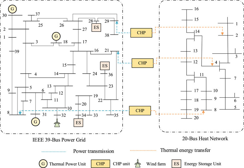
Figure 1. The tested system incorporating electricity and thermal system.

Figure 2

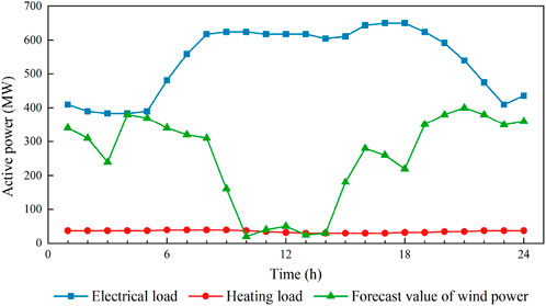
Figure 2. Predictive data of load and wind power.

5.1 Analysis of power system demand response results

This section analyzes the effect of price-based demand response for power systems, setting up the following two cases for comparative analysis:

Case 1.1. Power system load is fixed, regardless of demand response.

Case 1.2. Incorporating the price-based demand response within the power system, the load participating in the response accounts for 15% of the total load, ensuring that the energy is fixed throughout the day.

The electricity price is indicated in Table 1. The comparative outcomes of Case 1.1 and Case 1.2 are depicted in Figure 3.

Table 1

Table 1. Electricity price.

Figure 3

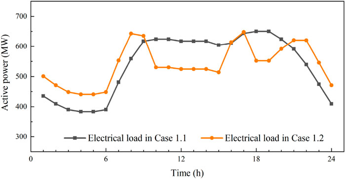
Figure 3. Electrical load before and after price-based demand response.

Figure 3 shows the electric load curves of Case 1.1 and Case 1.2. After considering the effect of price-based demand response, the peak-to-valley variance in electric load decreases from 266.5 MW in Case 1.1–207.3 MW in Case 1.2, which indicates that the demand response makes the electric load curve of the system smoother to some extent. The price-based demand response tends to make customers choose a more economical energy solution through price guidance, thus shifting portion of the peak load transitioning to the valley, making the valley load higher and the peak load lower, which effectively reduces transmission blockage and avoids the system to operate in a less efficient state for a long time. In addition, price-based demand response makes the nighttime electric load higher, which facilitates the utilization of significant quantities of wind power at night, raising the efficiency of renewable energy utilization and improving the energy mix.

The subsequent sensitivity analysis explores the effect of varying levels of load participation in demand response on peak-to-valley variance and load fluctuation standard deviation. The varying levels of load participation in demand response are specifically 0%, 5%, 10%, 15%, and 20%.

It can be seen from Table 2 that as the proportions of the load participating in demand response increase, both the peak-to-valley variance and power variance in the power system decrease. This indicates that by effectively leveraging the peak-shaving and valley-filling effects of demand response resources, the fluctuations in the system’s power load become more gradual, leading to an overall improvement in system operation.

Table 2

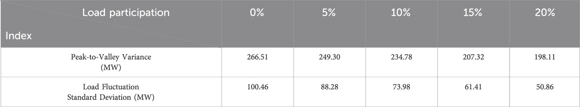
Table 2. The peak-to-valley variance and load fluctuation standard deviation under varying levels of load participation in demand response.

5.2 Analysis of thermal system heating demand adjustment results

To analyze the effect of regional thermal inertia on load regulation of thermal systems, the following two cases are set up in this section for comparison:

Case 2.1. The temperature of the heating area is fixed at 20°C.

Case 2.2. Heating area temperature is allowed to vary within 20°C ± 2°C.

The operation results of Case 2.1 and Case 2.2 are shown in Figures 4, 5.

Figure 4

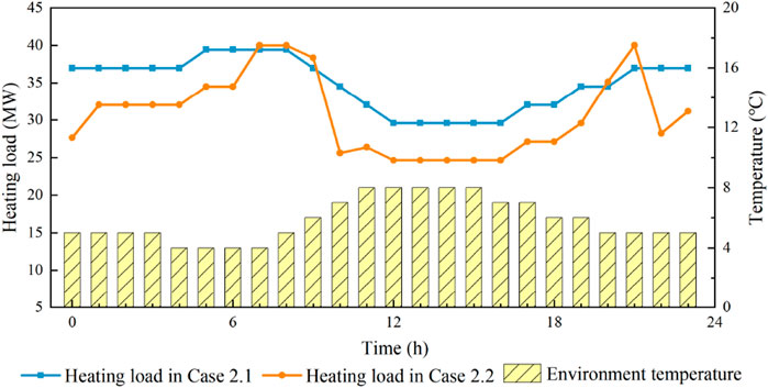
Figure 4. Heating load and environment temperature.

Figure 5

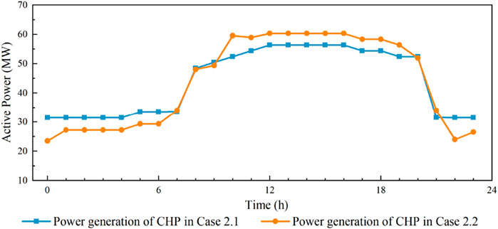
Figure 5. Power generation of CHP units.

According to the comparison of operation results in Figure 4, the heat load demand in Case 2.2 is lower than that in Case 2.1 during 0:00–6:00 and 22:00–23:00, which shows the temperature of the heating area in Case 2.2 is lower than 20°C. The thermal load reduction in this period has the following advantages: Firstly, the reduction of thermal load during this period can expand the power regulation range of CHP units, thus providing additional power reduction space for CHP units, which is conducive to increasing the wind power consumption at night. Secondly, the reduction of heat supply and electricity generation of CHP units reduces the fuel consumption of CHP units, which can improve the economy of system operation. In addition, the heat load increases during the 7:00–9:00 h. This is due to the large downward fluctuations in wind power output during the 9:00–10:00 h. The thermal system uses the thermal inertia of the heating area to store heat, which can increase the allowable drop in heat supply, and allow the CHP units to have a larger increase in power generation during this time period, as shown in Figure 5. As a result, the system can better cope with the power fluctuations. However, the adjustment of the thermal load affects the energy experience of users to some extent, so some financial compensation to the user is required.

5.3 Analysis of multi-type demand response results between electric and thermal energy sources

To assess the influence of multiple types of demand response on the operation of integrated electricity and thermal system, two distinct scenarios are established for comparative analysis in this section:

Case 3.1. No demand adjustment for electrical and thermal energy, and the model does not contain the electric heat pump unit.

Case 3.2. Consider the demand response of electric and thermal energy, and add electric heat pumps to the model for the conversion of energy between electrical and thermal forms.

The operating costs and wind abandonment of Case 3.1 and Case 3.2 are shown in the following table.

Based on the information provided in Table 3, it can be seen that the scheduling strategy that considers multiple types of demand response can significantly lower the operating cost of the system. The scheduling strategy can guide customers to choose more economical energy consumption solutions through energy prices, which reduce the electricity purchase costs of users. At the same time, the change of energy demand can also promote the consumption of wind power, effectively reduce the operation cost of generating units, and enhance the energy utilization rate.

Table 3

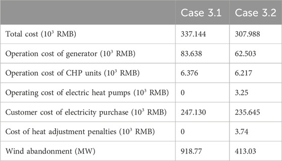
Table 3. Operating costs and wind abandonment.

In Case 3.2, electricity and heat energy are converted in both directions through CHP units and electric heat pumps to achieve mutual supplementation between different energy sources, and the scheduling results are shown in Figure 6.

Figure 6

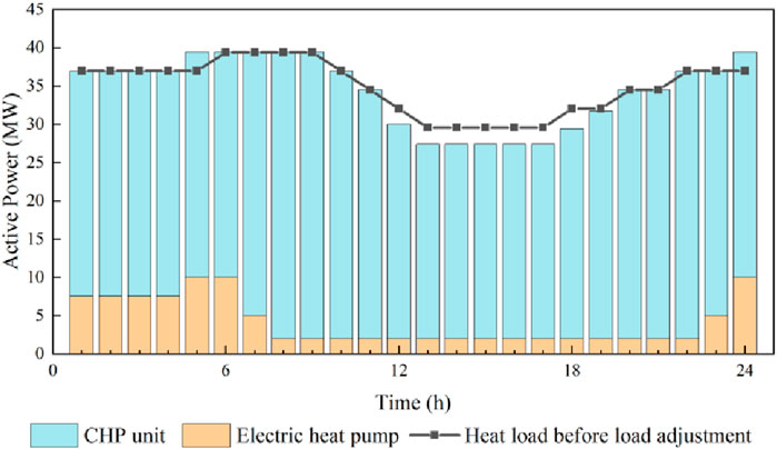
Figure 6. Heat source output condition in Case 3.2.

As can be seen from Figure 6, the heat load curves in Case 3.1 and Case 3.2 are basically the same. Since Case 3.1 does not contain an electric heat pump unit, its heat supply is all borne by the CHP unit. The heat demand of Case 3.2 is supplied by both CHP units and electric heat pumps. The electric heat pump has a higher output during the period of large wind abandonment at night. On the one hand, it increases the demand for electric energy and promotes the consumption of wind power. On the other hand, it makes up for the shortage of heat supply and reduces the influence on the energy comfort of users. In addition, the high level of electric heat pump output reduces the heat supply of CHP units, which provides more space for downward adjustment of CHP units’ power generation and further promotes wind power consumption. During the hours of peak electricity demand, the electric heat pump works at the lowest output level, and the heat energy is mainly provided by the CHP unit. The reduction in heat supply from the CHP unit provides more room for upward adjustment of the CHP unit’s power generation, which can better meet the demand of power consumption during that period.

6 Conclusion

This paper proposes a day-ahead optimal dispatching strategy for integrated electricity and thermal system considering multiple types of demand response, and the following conclusions emerge from the analysis of the price-based demand response, the thermal inertia of the heating system, and the conversion of electric and thermal energy.

The implementation of a price-based demand response in the power system encourages customers to opt for more economical energy consumption solutions guided by pricing signals. This approach successfully achieves peak reduction and valley filling effects, particularly by promoting wind power consumption at night. This strategy effectively alleviates the strain on the power grid during peak hours, contributing to a more sustainable and balanced energy utilization.

Coordinating the regional thermal inertia of the thermal system with CHP units proves instrumental. This coordination expands the controllable range of CHP unit power generation without compromising energy comfort. Additionally, it enables a swift response to wind power fluctuations, ensuring a more adaptable and resilient power generation system.

The scheduling strategy, accounting for multi-type demand responses, not only effectively reduces the operating cost of the system but also fosters increased consumption of wind power, thereby enhancing energy efficiency. The harmonized management of electric and thermal energy mitigates the impact of load adjustments on user energy comfort, ultimately optimizing the overall energy supply of the system.

Data availability statement

The raw data supporting the conclusion of this article will be made available by the authors, without undue reservation.

Author contributions

SS: Conceptualization, Writing–original draft. YC: Formal Analysis, Methodology, Writing–review and editing. JX: Writing–review and editing, Data curation. PY: Writing–review and editing, Formal analysis. YW: Writing–review and editing, Visualization.

Funding

The author(s) declare financial support was received for the research, authorship, and/or publication of this article. This work was supported by the Science and technology project of State Grid Shandong Electric Power Company (the Research on situation awareness and Energy Efficiency Online Evaluation Technology of integrated energy system, No. 52062622000S).

Conflict of interest

Authors SS, YC, JX, PY, and YW were employed by Electric Power Research Institute State Grid Shandong Electric Power Company.

The authors declare that this study received funding from State Grid Shandong Electric Power Company. The funder had the following involvement in the study: study design, collection, analysis, interpretation of data.

Publisher’s note

All claims expressed in this article are solely those of the authors and do not necessarily represent those of their affiliated organizations, or those of the publisher, the editors and the reviewers. Any product that may be evaluated in this article, or claim that may be made by its manufacturer, is not guaranteed or endorsed by the publisher.

References

Bai, L., Li, F., Cui, H., Jiang, T., Sun, H., and Zhu, J. (2016). Interval optimization based operating strategy for gas-electricity integrated energy systems considering demand response and wind uncertainty. Appl. energy 167, 270–279. doi:10.1016/j.apenergy.2015.10.119

CrossRef Full Text | Google Scholar

Cui, Y., Zhang, J., Wang, Z., Wang, T., and Zhao, Y. (2020). Day-ahead scheduling strategy of wind-PV-CSP hybrid power generation system by considering PDR. Proc. Chin. Soc. Electr. Eng. 40 (10), 3103–3114. (Chinese). doi:10.13334/j.0258-8013.pcsee.191388

CrossRef Full Text | Google Scholar

Feng, C., Wen, F., You, S., Li, Z., Shahnia, F., and Shahidehpour, M. (2019). Coalitional game-based transactive energy management in local energy communities. IEEE Trans. Power Syst. 35 (3), 1729–1740. doi:10.1109/tpwrs.2019.2957537

CrossRef Full Text | Google Scholar

Fu, L., Liu, B., Meng, K., and Dong, Z. Y. (2020). Optimal restoration of an unbalanced distribution system into multiple microgrids considering three-phase demand-side management. IEEE Trans. Power Syst. 36 (2), 1350–1361. doi:10.1109/tpwrs.2020.3015384

CrossRef Full Text | Google Scholar

Huang, W., Zhang, N., Kang, C., Li, M., and Huo, M. (2019). From demand response to integrated demand response: review and prospect of research and application. Prot. Control Mod. Power Syst. 4, 12–13. doi:10.1186/s41601-019-0126-4

CrossRef Full Text | Google Scholar

International Energy Agency (2020). Renewables 2020 [EB/OL]. Available at: https://www.iea.org/reports/renewables-2020?language=zh (Accessed March 07, 2022).

Google Scholar

Li, J., Fang, J., Zeng, Q., and Chen, Z. (2016a). Optimal operation of the integrated electrical and heating systems to accommodate the intermittent renewable sources. Appl. Energy 167, 244–254. doi:10.1016/j.apenergy.2015.10.054

CrossRef Full Text | Google Scholar

Li, J., and Hu, L. (2015). Research on accommodation scheme of curtailed wind power based on peak-shaving electric boiler in secondary heat supply network. Power Syst. Technol. 39 (11), 3286–3291. (Chinese). doi:10.13335/j.1000-3673.pst.2015.11.041

CrossRef Full Text | Google Scholar

Li, Y., Wang, C., Li, G., and Chen, C. (2021). Optimal scheduling of integrated demand response-enabled integrated energy systems with uncertain renewable generations: a Stackelberg game approach. Energy Convers. Manag. 235, 113996. doi:10.1016/j.enconman.2021.113996

CrossRef Full Text | Google Scholar

Li, Y., Yang, Z., Li, G., Mu, Y., Zhao, D., Chen, C., et al. (2018). Optimal scheduling of isolated microgrid with an electric vehicle battery swapping station in multi-stakeholder scenarios: a bi-level programming approach via real-time pricing. Appl. energy 232, 54–68. doi:10.1016/j.apenergy.2018.09.211

CrossRef Full Text | Google Scholar

Li, Z., Wu, W., Wang, J., Zhang, B., and Zheng, T. (2016b). Transmission-Constrained unit commitment considering combined electricity and district heating networks. IEEE Trans. Sustain. Energy 7 (2), 480–492. doi:10.1109/TSTE.2015.2500571

CrossRef Full Text | Google Scholar

Lin, Z., Jiang, F., Luo, Y., Liu, K., and Zhang, X. (2022). Data-driven situation awareness of electricity-gas integrated energy system considering time series features. Front. Energy Res. 10, 10. doi:10.3389/fenrg.2022.921296

CrossRef Full Text | Google Scholar

Liu, D., Sun, Y., Li, B., Xiangying, X., and Yudong, L. (2020). Differentiated incentive strategy for demand response in electric market considering the difference in user response flexibility. IEEE Access 8 (1), 17080–17092. doi:10.1109/access.2020.2968000

CrossRef Full Text | Google Scholar

Liu, P., Ding, T., Zou, Z., and Yang, Y. (2019). Integrated demand response for a load serving entity in multi-energy market considering network constraints. Appl. Energy 250, 512–529. doi:10.1016/j.apenergy.2019.05.003

CrossRef Full Text | Google Scholar

Long, H., Fu, L., and Xu, R. (2015). Research on the electric grid dispatch for alleviating the uncertainties impact through gas-fired cogenerations and heat pumps. Trans. China Electrotech. Soc. 30 (20), 219–226. (Chinese). doi:10.19595/j.cnki.1000-6753.tces.2015.20.027

CrossRef Full Text | Google Scholar

Meibom, P., Kiviluoma, J., Barth, R., Brand, H., Weber, C., and Larsen, H. V. (2007). Value of electric heat boilers and heat pumps for wind power integration. Wind Energy Int. J. Prog. Appl. Wind Power Convers. Technol. 10 (4), 321–337. doi:10.1002/we.224

CrossRef Full Text | Google Scholar

Nuytten, T., Claessens, B., Paredis, K., Van Bael, J., and Six, D. (2013). Flexibility of a combined heat and power system with thermal energy storage for district heating. Appl. Energy 104, 583–591. doi:10.1016/j.apenergy.2012.11.029

CrossRef Full Text | Google Scholar

Wang, B., Li, Y., Ming, W., and Wang, S. (2020). Deep reinforcement learning method for demand response management of interruptible load. IEEE Trans. Smart Grid 11 (4), 3146–3155. doi:10.1109/tsg.2020.2967430

CrossRef Full Text | Google Scholar

Wang, J., Mohammad, S., and Li, Z. (2008). Security-constrained unit commitment with volatile wind power generation. IEEE Trans. Power Syst. 23 (03), 1319–1327. doi:10.1109/tpwrs.2008.926719

CrossRef Full Text | Google Scholar

Wang, J., Zhong, H., Ma, Z., Xia, Q., and Kang, C. (2017). Review and prospect of integrated demand response in the multi-energy system. Appl. Energy 202, 772–782. doi:10.1016/j.apenergy.2017.05.150

CrossRef Full Text | Google Scholar

Wang, K., Wang, C., Zhang, Z., and Wang, X. (2022). Multi-timescale active distribution network optimal dispatching based on SMPC. IEEE Trans. Industry Appl. 58 (2), 1644–1653. doi:10.1109/tia.2022.3145763

CrossRef Full Text | Google Scholar

Wang, S., Bi, S., and Zhang, Y. J. A. (2018). Demand response management for profit maximizing energy loads in real-time electricity market. IEEE Trans. Power Syst. 33 (6), 6387–6396. doi:10.1109/tpwrs.2018.2827401

CrossRef Full Text | Google Scholar

Xia, T., Li, Y., Zhang, N., and Kang, C. (2022). Role of compressed air energy storage in urban integrated energy systems with increasing wind penetration. Renew. Sustain. Energy Rev. 160, 112203. doi:10.1016/j.rser.2022.112203

CrossRef Full Text | Google Scholar

Xu, H., Dong, S., He, Z., Shi, Y., Wang, L., and Liu, Y. (2019). Electro-thermal comprehensive demand response based on multi-energy complementarity. Power Syst. Technol. 43 (02), 480–489. (Chinese). doi:10.13335/j.1000-3673.pst.2018.2234

CrossRef Full Text | Google Scholar

Yi, Z., and Li, Z. (2018). Combined heat and power dispatching strategy considering heat storage characteristics of heating network and thermal inertia in heating area. Power Syst. Technol. 42 (05), 1378–1384. (Chinese). doi:10.13335/j.1000-3673.pst.2017.2703

CrossRef Full Text | Google Scholar

Zhang, Z., Wang, C., Wang, R., Guo, G., Chen, S., and Wang, Y. (2021). “Multi-time scale Co-optimization scheduling of integrated energy system for uncertainty balancing,” in 2021 IEEE/IAS Industrial and Commercial Power System Asia, Chengdu, China, July 2021 (I&CPS Asia), 270–276. doi:10.1109/ICPSAsia52756.2021.9621574

CrossRef Full Text | Google Scholar